Integrating Temperature History into Inherent Strain Methodology for Improved Distortion Prediction in Laser Powder Bed Fusion

Abstract

Powder bed fusion–laser beam (PBF-LB) additive manufacturing enables the production of intricate, lightweight metal components aligned with Industry 4.0 and sustainable principles. However, residual stresses and distortions challenge the dimensional accuracy and reliability of parts. Inherent strain methods (ISMs) provide a computationally efficient approach to predicting these issues but often overlook transient thermal histories, limiting their accuracy. This paper introduces an enhanced inherent strain method (EISM) for PBF-LB, integrating macro-scale temperature histories into the inherent strain framework. By incorporating temperature-dependent adjustments to the precomputed inherent strain tensor, EISM improves the prediction of residual stresses and distortions, addressing the limitations of the original ISM. Validation was conducted on two Ti-6Al-4V geometries—a non-symmetric bridge and a complex structure (steady blowing actuator)—through comparisons with experimental measurements of temperature, distortion, and residual stress. Results demonstrate improved accuracy, particularly in capturing localized thermal and mechanical effects. Sensitivity analyses emphasize the need for adaptive layer lumping and mesh refinement in regions with abrupt stiffness changes, such as shrink lines. While EISM slightly increases computational cost, it remains feasible for industrial-scale applications. This work bridges the gap between simplified inherent strain models and high-fidelity simulations, offering a robust tool for simulation-driven optimisation.

1. Introduction

Powder Bed Fusion-Laser Beam (PBF-LB) has emerged as a transformative technology in metal Additive Manufacturing (AM), offering the unique ability to fabricate highly complex and optimised components directly from digital designs. PBF-LB aligns with the principles of Industry 4.0, providing industries such as the aerospace, defense, automotive, and healthcare sectors with tools to create lightweight, high-performance components while minimizing material waste and production time [1,2]. The technology’s ability to support topology-optimised designs and intricate geometries has made it a key driver of innovation across these sectors [3]. PBF-LB also offers notable environmental advantages. The process is inherently material efficient, using only the necessary amount of metal powder for fabrication, with excess material often being recyclable [4,5]. These factors collectively support sustainable manufacturing principles, aligning with global efforts to minimize the environmental impact of industrial processes.

Despite its transformative potential, PBF-LB faces persistent residual stresses and distortions challenges. These issues arise from the rapid thermal cycles, steep temperature gradients, and complex phase transformations that are intrinsic to the layer-by-layer deposition process [6,7]. They can not only compromise the dimensional accuracy and structural integrity of manufactured components but also pose barriers to the widespread adoption of PBF-LB in high-value industrial applications. Addressing these challenges requires robust predictive tools capable of capturing the multi-physics nature of the process, including thermal, mechanical, and metallurgical interactions.

Physics-based numerical simulations have become indispensable for understanding the complex phenomena underlying the PBF-LB process and for guiding process parameter optimisation. These techniques enable detailed analysis of thermal, mechanical, and metallurgical interactions that govern the quality and performance of manufactured components [8]. Among these methods, the Inherent Strain Method (ISM) has emerged as a computationally efficient alternative for predicting residual stresses and distortions in PBF-LB. Originally developed for welding processes [9], ISM was adapted for additive manufacturing due to its ability to approximate complex thermo-mechanical interactions using predefined strain fields. This simplification allows ISM to achieve significant reductions in computational cost, making it attractive for industrial-scale problems, where computational resources are often a limiting factor. Studies by Mohammadtaheri et al. [10] and Bayat et al. [11] highlight the widespread adoption of ISM in PBF-LB modelling, particularly in predicting distortions and optimising process parameters. Additionally, these studies highlight the successful integration of ISM into commercial software platforms, boosting its use in industrial applications.

Surrogate modelling has recently become an interesting tool to accelerate the simulation process even further [12]. Indeed, it has been used in combination with inherent strain numerical models to generate the required datasets for training, ultimately resulting in almost instantaneous predictors that can be successfully applied even in design optimisation [13]. Improving inherent strain-based modelling methodologies not only enhances predictive accuracy but also improves the quality of datasets used to train surrogate models, thereby advancing their reliability for PBF-LB applications.

The ISM, in its original and most widely adopted form, provides a simplified yet practical approach to modelling the residual stresses and deformations that arise during metal AM. Its implementation is thoroughly documented in the literature [9,14,15]. Broadly speaking, the methodology involves a sequence of mechanical, linear elastic simulation steps combined with a prescribed activation strategy. Typically, the simulation proceeds layer-by-layer, and at each simulation step, a new layer is activated, and the inherent strain is applied. Multiple layers are often lumped and activated simultaneously, thereby reducing the number of incremental steps as well as the total number of elements, which ultimately decreases the overall computational cost. The inherent strain tensor can be experimentally calibrated by measuring distortions in test coupons [15] or can be derived from high-fidelity thermo-mechanical simulations at the meso-scale [16].

Over time, refinements in ISM have emerged to improve accuracy in residual stress and deformation predictions [17,18,19]. These advancements primarily focus on refining the methods used to derive inherent strains from local thermo-mechanical models.

The original ISM assumes that each deposited layer inherits a constant inherent strain state, neglecting spatial and temporal variations in the thermal field. While this assumption enables large computational savings, it may oversimplify the process physics, particularly in parts featuring non-uniform geometries or complex scanning strategies where steep thermal gradients may occur. Consequently, conventional ISM frameworks might struggle to predict residual stresses and distortions accurately in certain scenarios [20]. Addressing these shortcomings is crucial for advancing the fidelity and reliability of ISM in PBF-LB applications.

Recent efforts have begun to address this limitation by including local thermal histories into the ISM [19,21]. For instance, Pourabdollah et al. [22] introduced a variant of the ISM tailored for Electron beam powder bed fusion (PBF-EB), which accounts for both compressive plastic strains adjacent to the melt pool and thermal strains associated with the evolving macroscale thermal field during fabrication. Although PBF-LB differs from PBF-EB in some aspects, the underlying challenges of representing localized temperature gradients and their influence on residual stresses remain comparable. This insight motivates extending thermal-history-informed ISM variants to the PBF-LB context.

In this paper, we present an Enhanced Inherent Strain Method (EISM) for PBF-LB, which integrates part-scale temperature evolution into the original ISM. Unlike high-fidelity thermo-mechanical analysis, this approach computes only the average temperature field evolution, which is largely influenced by the part geometry and boundary conditions. While the starting point of the EISM remains a precomputed inherent strain tensor (including thermal, plastic, and other strain components) as in ISM, this is further adjusted based on the computed part-scale temperature history. This adaptation provides a more physically realistic representation of the deformation mechanisms by accounting for the geometry- and boundary-condition-induced effects on thermal behaviour.

The findings of this study are particularly relevant to engineers, researchers, and industrial practitioners working to optimise PBF-LB processes. Engineers and researchers can leverage the proposed modelling advancements to refine process parameters for specific geometries and boundary conditions, thereby reducing distortions and residual stresses. Industrial practitioners can integrate these methodologies into simulation-driven design workflows to predict and mitigate manufacturing defects. Furthermore, these improvements in inherent strain-based modelling enhance the quality of training datasets for surrogate models, ultimately contributing to more efficient and accurate design optimisation.

In summary, this work aims to enhance the accuracy and practicality of the ISM for PBF-LB by integrating part-scale thermal histories into the framework, resulting in an EISM. The specific objectives are to

• Develop the EISM: incorporate thermal history effects to improve the physical accuracy of residual stress and distortion predictions.
• Validate predictive accuracy: compare EISM and ISM results with experimental data for parts with complex thermal gradients.
• Assess computational efficiency: evaluate and compare the computational cost and performance of ISM and EISM.

The remainder of this paper is organized as follows:

• Modelling Approach (Section 2) details the enhanced inherent strain modelling approach, including how macro-scale thermal histories are integrated into the original ISM framework.
• Experimental Campaign for Calibration and Validation (Section 3) describes the experimental campaign, including the tested geometries, materials, process parameters, and measurement techniques used for calibration and validation.
• Numerical Implementation (Section 4) presents the numerical implementation of the EISM in the selected testing geometries, including mesh generation, boundary conditions, and computational settings.
• Results and Discussion (Section 5) compares EISM and ISM predictions with experimental data, discussing the effects of mesh size, layer lumping, and computational efficiency.
• Conclusions (Section 6) summarizes the key findings and outlines future research directions.

By addressing these objectives, this study advances the predictive accuracy and applicability of simulation-based process optimisation in PBF-LB.

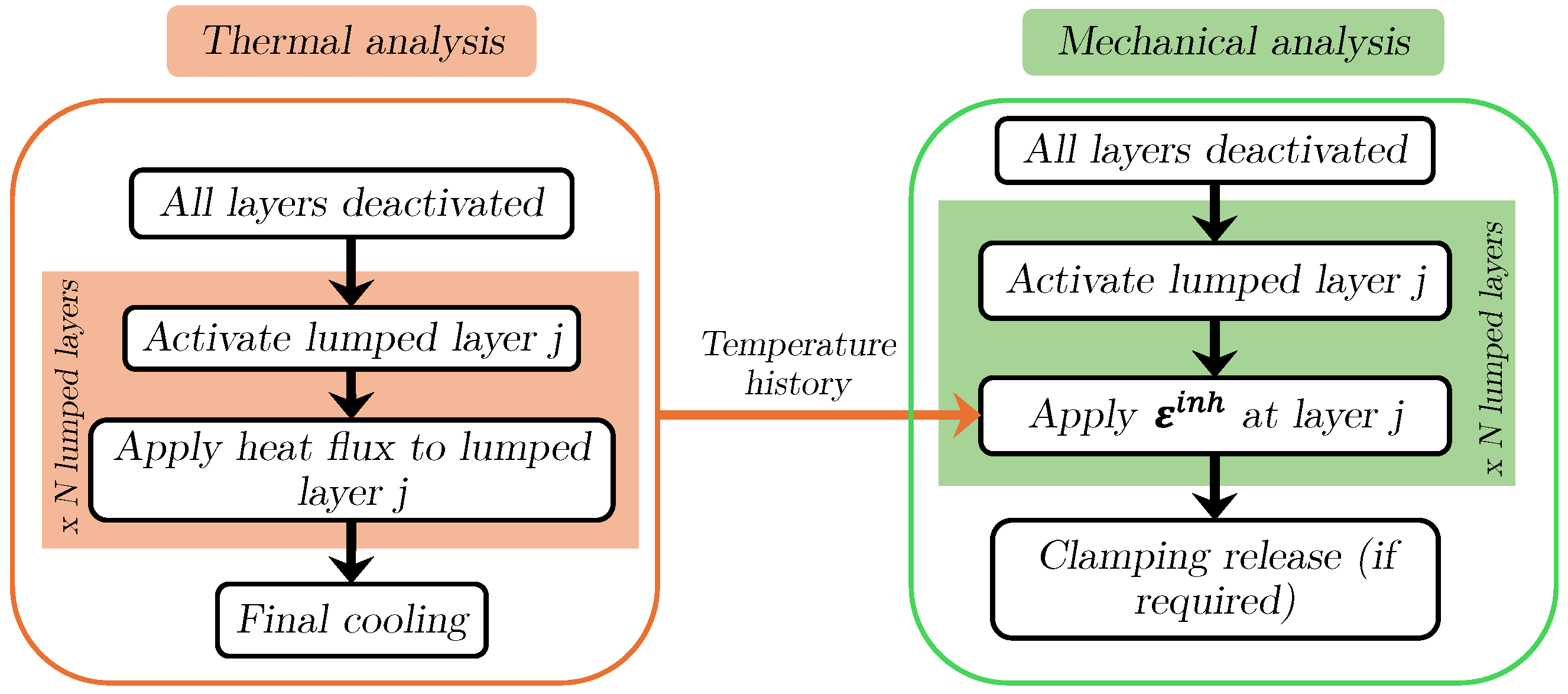
2. Modelling Approach

The EISM is a sequentially coupled layer-by-layer thermo-mechanical analysis method. A general overview of the methodology is illustrated in Figure 1. The following subsections detail the key considerations and the overall solution procedure.

2.1. Thermal Analysis

The layer-by-layer macro-scale thermal model follows the approach outlined in previous studies [23]. In this work, it is used to calculate the average temperature field evolution of the printed domain before the subsequent layer is deposited.

The heat transfer within the domain is governed by the transient heat conduction equation:

$$\rho c_p{\displaystyle \frac{\partial T}{\partial t}}=\nabla ·(k\nabla T)+\dot{Q}$$

(1)

where $\rho$ is the material density, $c_p$ is the specific heat capacity, T is the temperature, t is time, k is the thermal conductivity, and $\dot{Q}$ represents heat rate generation per unit volume, including heat input from the laser or other energy sources.

To reduce computational time, several layers can be lumped together, and a time-averaged volumetric heat source, $\dot{Q}$, is applied to the entire volume of the lumped layers during an equivalent time step. The time step for the j-th lumped layer is computed as

$$\Delta t_j=\sum _{i=n·(j-1)+1}^{n·j}\left(t_i^{laser}+t_i^{recoater}\right)$$

(2)

where i is the layer counter, n is the number of layers in each lump, and $t_i^{laser}$ and $t_i^{recoater}$ correspond to the laser exposure and recoating times for layer i, respectively.

The time-averaged heat source is computed within the FEM framework by modelling the moving heat source as a “concentrated moving heat source” [24,25]. Using this approach, the energy input to the system is determined based on the scanning sequence. During each time step, the algorithm identifies all elements intersected by the laser and applies the corresponding heat flux to these elements. This method accounts for different scanning patterns and process parameters for each layer, offering the flexibility needed to accurately simulate diverse additive manufacturing process conditions.

Heat losses at the boundaries are modelled via convection and radiation.

• Convection: $q=h(T-T_{\infty })$, where h is the heat transfer coefficient, and $T_{\infty }$ is the ambient temperature.
• Radiation: $q=ϵ\sigma (T^4-T_{\infty }^4)$, where $ϵ$ is the emissivity, and $\sigma$ is the Stefan–Boltzmann constant.

2.2. Mechanical Analysis

The mechanical equilibrium is described by the quasi-static balance of momentum equation:

$$\nabla ·\mathit{\sigma }+\mathit{b}=0$$

(3)

where $\mathit{\sigma }$ is the Cauchy stress tensor and $\mathit{b}$ represents body forces per unit volume.

The constitutive relationship of the material is

$$\sigma =\mathit{C}:{\mathit{\epsilon }}^e$$

(4)

where $\mathit{C}$ is the fourth-order constitutive tensor, and ${\mathit{\epsilon }}^e$ is the elastic strain tensor.

Under the assumptions of small strain theory, the elastic strain tensor can be computed as

$${\mathit{\epsilon }}^e={\mathit{\epsilon }}^{total}-{\mathit{\epsilon }}^{inh}$$

(5)

where ${\mathit{\epsilon }}^{total}={\nabla }^s\left(\mathit{u}\right)$ is the total strain tensor, and ${\mathit{\epsilon }}^{inh}$ is the inherent strain tensor.

2.3. EISM Considerations

The inherent strain tensor includes all non-elastic strain components. It is defined as

$${\mathit{\epsilon }}^{inh}={\mathit{\epsilon }}^{total}-{\mathit{\epsilon }}^e={\mathit{\epsilon }}^{th}+{\mathit{\epsilon }}^{pl}+{\mathit{\epsilon }}^{act}$$

(6)

where ${\mathit{\epsilon }}^{th}$ is the thermal strain tensor, ${\mathit{\epsilon }}^{pl}$ is the plastic strain tensor, and ${\mathit{\epsilon }}^{act}$ is the activation strain tensor.

${\mathit{\epsilon }}^{inh}$ can be obtained through either meso-scale thermo-mechanical simulations or experimental calibration [15,16]. This precomputed inherent strain tensor will hereafter be denoted as ${\mathit{\epsilon }}^{inh,0}$ and is subsequently used as input data in methodologies based on inherent strain theory.

In the original ISM, ${\mathit{\epsilon }}^{inh}$ is assumed to be constant for each material point and is applied at the moment of material deposition:

$${\mathit{\epsilon }}^{inh}={\mathit{\epsilon }}^{inh,0}$$

(7)

The EISM enhances the original approach by incorporating temperature dependence. The scope is to make ${\mathit{\epsilon }}^{inh}$ both temperature and time dependent, using the average temperature of the deposited domain. Consequently, ${\mathit{\epsilon }}^{inh,0}$ is enhanced with the thermal strain history calculated in the layer-by-layer macro-scale thermal analysis (as detailed in Section 2.1). Thus, the inherent strain ${\mathit{\epsilon }}^{inh}$ applied in EISM is expressed as

$${\mathit{\epsilon }}^{inh}={\mathit{\epsilon }}^{inh,0}+\Delta {\mathit{\epsilon }}^{th}$$

(8)

The layer lumping strategy should be applied carefully, as plastic strain typically stabilizes only after several layers have been deposited, as demonstrated in [16]. Since the objective is to enhance ${\mathit{\epsilon }}^{\mathit{inh},0}$ while preserving the plastic and activation components unchanged, the minimum number of layers to be considered in the calculations must be carefully determined.

The thermal strain depends on the thermal field and is computed as

$${\mathit{\epsilon }}^{th}=[\alpha \left(T\right)·(T-T_{ref})-\alpha \left(T_0\right)·(T_0-T_{ref})]\mathit{I}$$

(9)

where T is the current temperature, $\alpha \left(T\right)$ is the temperature-dependent secant thermal expansion coefficient, $T_{ref}$ is the reference temperature for the expansion coefficient, and $T_0$ is the initial temperature of the material at the start of the simulation.

Note that ${\mathit{\epsilon }}^{inh,0}$ typically accounts for the total thermal deformation during the cooling procedure. Thus, for $T=T_{\mathit{ref}}$, the deformation reaches its maximum value:

$${\mathit{\epsilon }}^{th,0}=[-\alpha \left(T_0\right)·(T_0-T_{ref})]\mathit{I}$$

(10)

However, the thermal analysis provides the temperature field of the component just before the deposition of the next (lumped) layer. The temperature distribution is generally non-uniform in space, depending on the specific scanning pattern, geometry, and boundary conditions. Therefore, the actual thermal deformation is recovered by EISM by including the missing contribution $\Delta {\mathit{\epsilon }}^{th}$, defined as

$$\Delta {\mathit{\epsilon }}^{th}=[\alpha \left(T\right)·(T-T_{ref})]\mathit{I}$$

(11)

Thus, the ${\mathit{\epsilon }}^{inh}$ applied in EISM is

$${\mathit{\epsilon }}^{inh}={\mathit{\epsilon }}^{inh,0}+[\alpha \left(T\right)·(T-T_{ref})]\mathit{I}$$

(12)

where T is the current temperature at the component.

It is important to note that at the end of the process, when all material points reach the reference temperature, $\Delta {\mathit{\epsilon }}^{th}$ reduces to zero, and the applied ${\mathit{\epsilon }}^{inh}$ aligns with that of the ISM.

Additionally, in EISM, material properties are considered temperature-dependent, marking another distinction from the original ISM. This temperature dependence leads to different behaviour of the deposited material as the process progresses.

2.4. Material Deposition Modelling

The material deposition approach employed in both the heat transfer and mechanical analyses is the birth–death element technique. In this approach, a new layer of elements is activated at each time step.

The activation strategy is carefully designed to address the behaviour of inactive elements that share nodes with active ones. In the heat transfer analysis, it is ensured that the temperature at the integration points of these inactive elements remains equal to the initial temperature specified at the nodes. This guarantees a smooth thermal transition and prevents unrealistic temperature gradients during activation.

Similarly, in the mechanical analysis, initial deformations may occur in inactive elements due to the displacement of shared nodes with active elements. To counteract this, activation strains are applied as described in [25,26]. These strains compensate for the deformations, ensuring that the newly activated elements are in a stress-free configuration upon activation. This approach maintains consistency in the mechanical response and avoids introducing spurious residual stresses into the model.

3. Experimental Campaign for Calibration and Validation

The experimental campaign described in this section was conducted to provide the necessary data for the calibration and validation of numerical models used in inherent strain modelling. The experiments aim to capture critical thermal and mechanical behaviours during the manufacturing process, enabling a more accurate prediction of distortions and residual stresses. A detailed description of the experimental setup and results for the majority of the work is available in [16]. For completeness, a summary of the earlier work is provided here, along with details of additional distortion and residual stress measurements conducted for this study.

Two geometries, both manufactured using the Ti-6Al-4V alloy on an SLM 280 HL machine, were investigated:

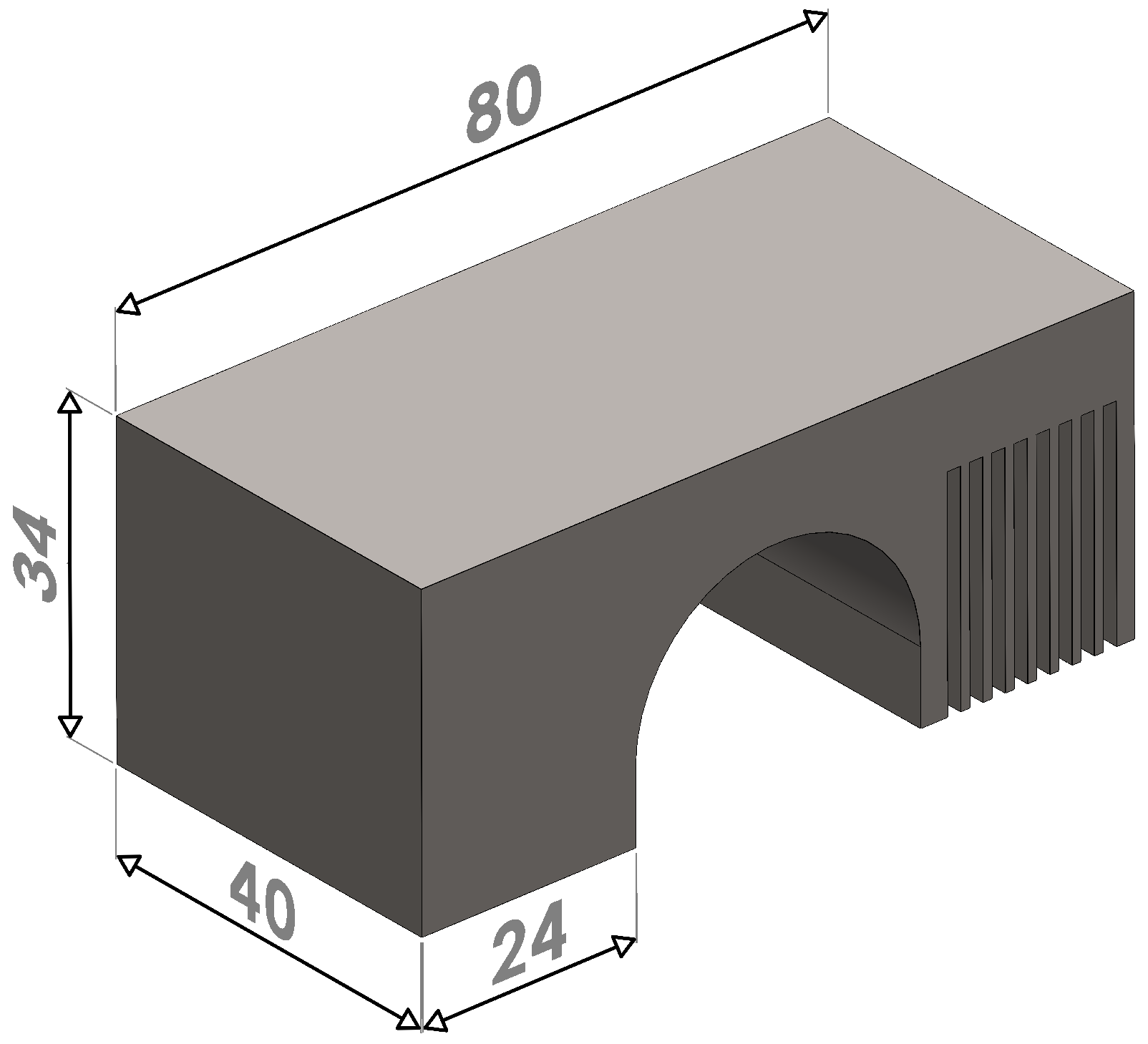
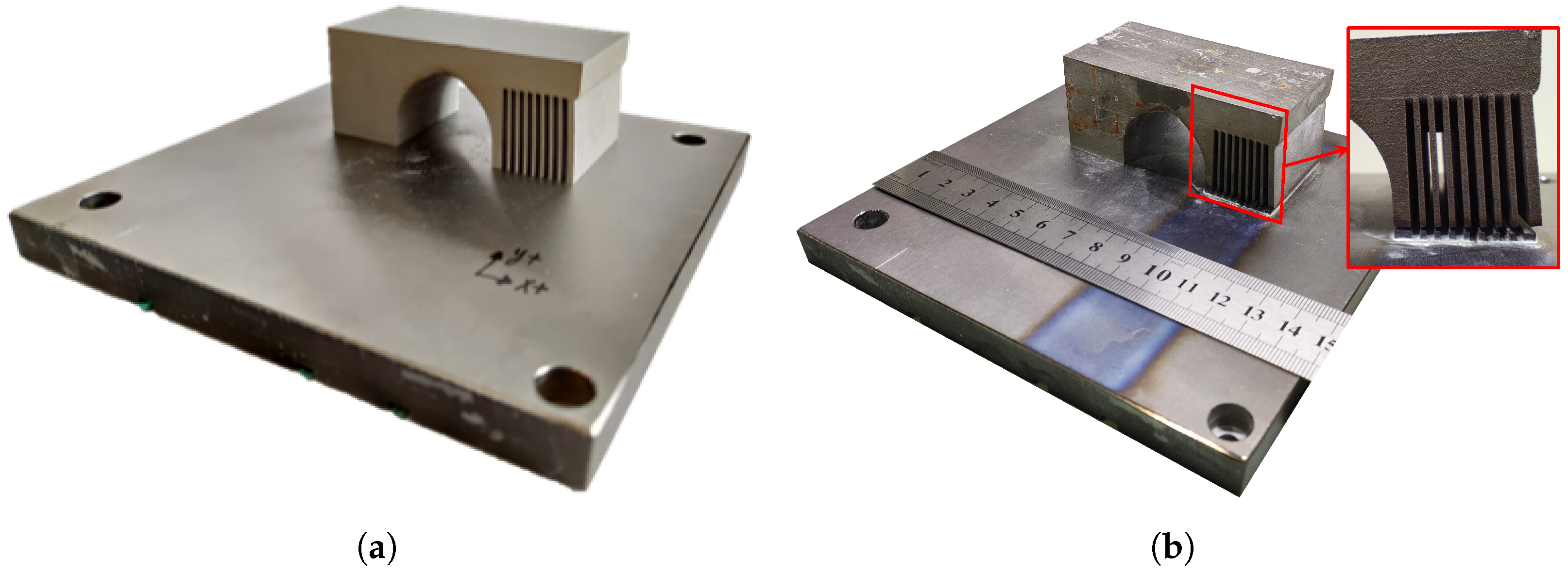
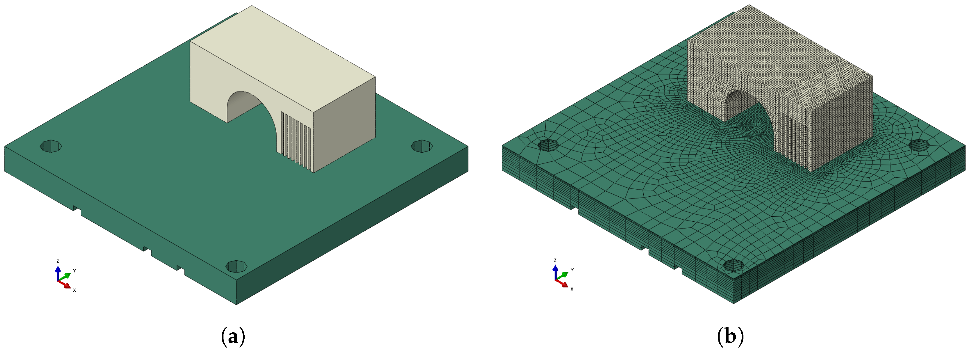
• The non-symmetric bridge geometry (Figure 2), chosen for its simplicity, allowed for an analysis of local temperature, distortion, and residual stress. It was manufactured on a baseplate with dimensions of $150\times 150\times 24{\mathrm{mm}}^3$.
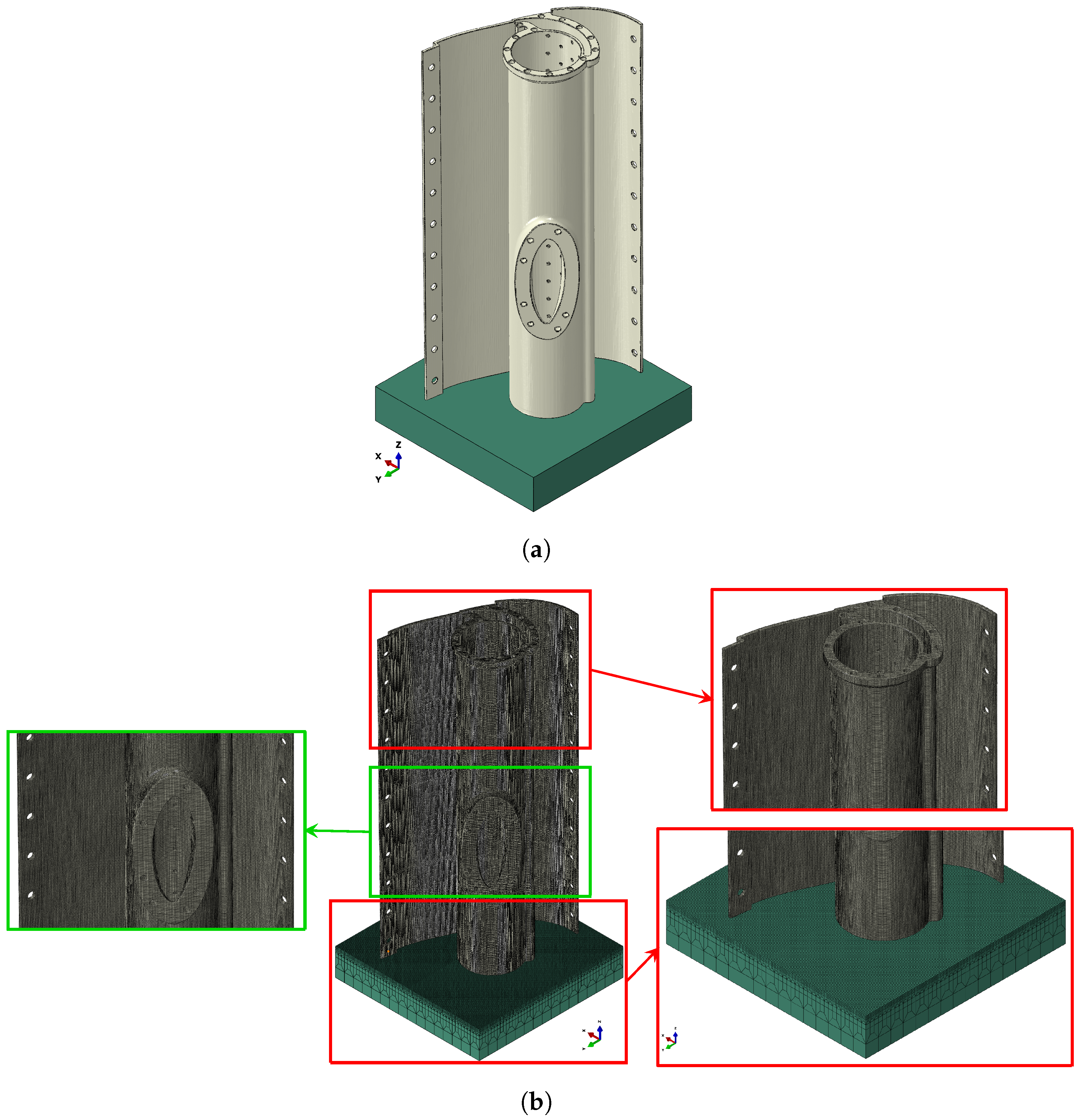
• The Steady Blowing Actuator (SBA) (Figure 3), representing a complex industrial application, was ideal for studying distortions in larger, more complex designs. It was manufactured on a baseplate with dimensions of $160\times 160\times 30{\mathrm{mm}}^3$.

Key process parameters were carefully optimised to ensure high-quality part fabrication, as detailed in [16]. To account for real process variations, laser exposure and recoating times were monitored (Figure 4). These measurements revealed significant deviations from theoretical values, which, if neglected, could have a substantial impact on the accuracy of the predicted temperature history.

Temperature measurements were conducted at six specific locations of the bridge using K-type thermocouples embedded in the baseplate (Figure 5). These measurements provided critical data for validating the macro-scale thermal models.

Distortion measurements were performed for both geometries. For the non-symmetric bridge, distortion was measured after printing along the front path depicted in Figure 6, without applying any stress relaxation treatment. Subsequently, the bridge was partially cut from the baseplate using wire Electrical Discharge Machining (wEDM) to release part of the residual stress. After cutting, the deflection of the top surface was measured along the top path shown in Figure 6. Figure 7 illustrates the state of the bridge before and after cutting. For the SBA geometry, the entire manufactured part was scanned with a 3D scanner to capture its deformed shape. This information was subsequently used to perform a detailed deviation analysis.

In addition, residual stress measurements were performed on the bridge using the incremental hole drilling technique, employing an MTS-3000 RS measurement machine and following the ASTM E837-13a standard. Measurements were taken at three points on different surfaces, as shown in Figure 8. This technique involved creating blind holes and measuring strain relief with a high-precision CEA-062UL-120 strain gauge, providing valuable insights into the distribution of residual stresses.

4. Numerical Implementation

This section outlines the numerical implementation of the EISM modelling approach for both geometries described in Section 3.

The Finite Element (FE) software employed for the simulations was ABAQUS. This software provides general-purpose finite element simulation capabilities as well as specialized tools for simulating additive manufacturing processes, which incorporate machine-specific information and process parameters.

All simulations were conducted using parallel computing with the linear iterative solver of ABAQUS/Standard, utilizing 24 CPUs (Intel Xeon E5-2690v3) and 192 GB of RAM.

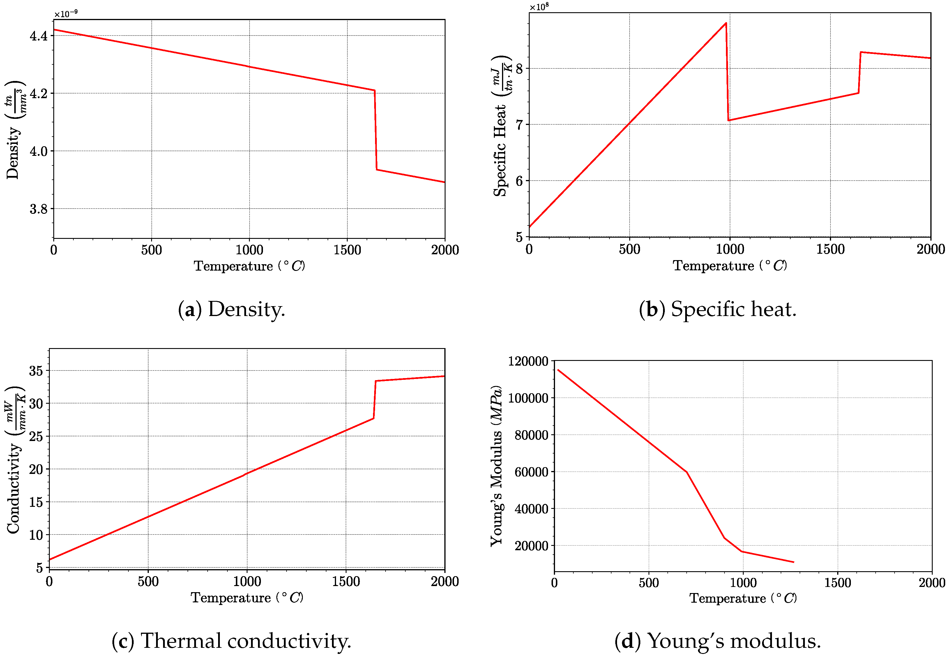
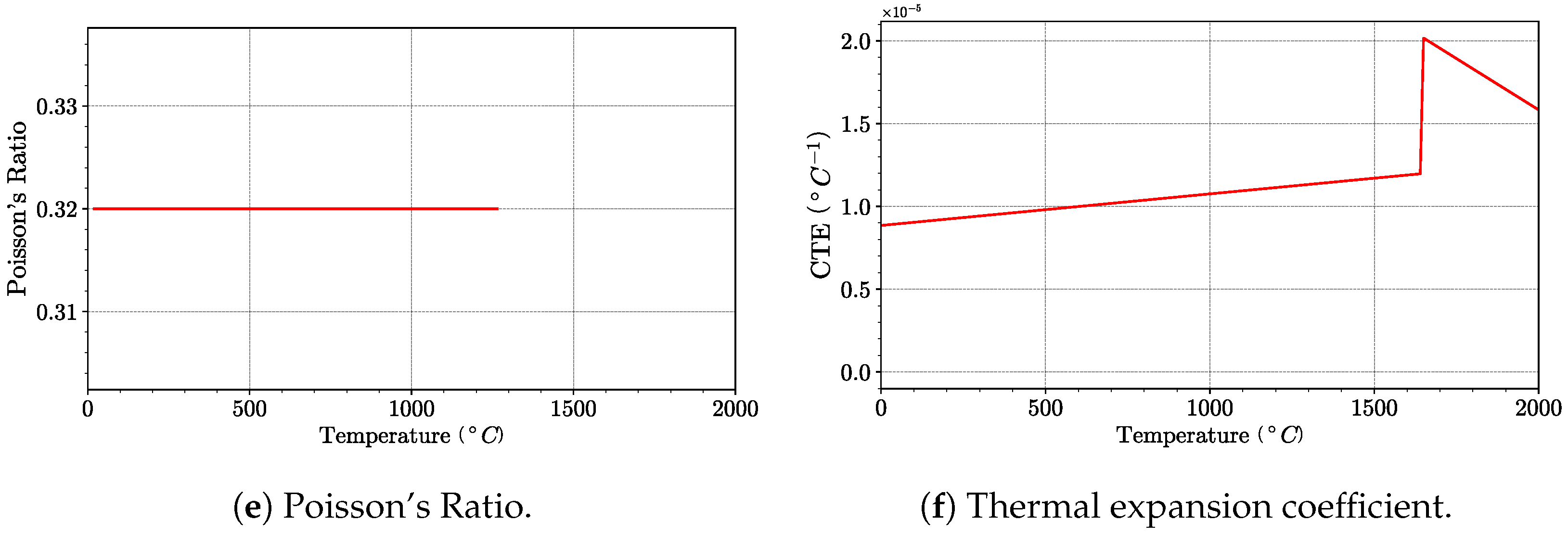
4.1. Material Properties

The material properties of the Ti-6Al-4V alloy were defined based on the literature [27]. Temperature-dependent material properties and a linear elastic material model were considered (see Figure A1) to ensure consistency between the local models used for inherent strain computation [16] and the part-scale models analysed in this paper.

It is essential to acknowledge the influence of material property dispersion on the physical properties of elements produced using PBF-LB. Anisotropy in mechanical properties, induced by factors such as scanning strategy, layer thickness, and build orientation, can significantly affect performance. To address these factors to some extent, the reliable source [27] was used, where material properties were obtained by averaging data from multiple references. Additionally, in-house experiments conducted by Ganeriwala et al. provided further insights to partially account for material property dispersion. However, the modelling scale and physics considered in these methodologies do not allow to predict texture or anisotropy.

The precomputed inherent strain tensor, ${\mathit{\epsilon }}^{inh,0}$, used in this study was directly adopted from [16]. In Voigt notation, the tensor is expressed as

$${\tilde{\mathit{\epsilon }}}^{inh}=-0.0056\left(\begin{array}{cccccc}1& 1& 0& 0& 0& 0\end{array}\right)$$

(13)

4.2. Geometrical Model and FE Mesh

Figure 9 and Figure 10 show the 3D geometrical domain and the corresponding FE global meshes for the non-symmetric bridge and the SBA, respectively. The baseplate was included in both models to account for the heat sink effect it induces during the simulation. Non-coincident meshes were employed for the printed parts and the baseplates, connected using a “Tie” constraint to ensure continuity in both temperature and displacements.

To analyze the effect of mesh size on simulation accuracy, two different meshes were defined for the non-symmetric bridge (see Figure 11), consistent with the lumping strategy. In the first mesh, the characteristic element size is approximately $0.24\mathrm{mm}$. This element size was selected based on the findings of a previous study described in [16], which concluded that a minimum lumping size of four layers is required to achieve plastic strain stabilization. This mesh ensures that at least one element exists per lumped layer, maintaining numerical accuracy. In the second mesh, a characteristic element size of $0.96\mathrm{mm}$ was used, allowing for a minimum lumping of 16 layers. This coarser mesh provides a comparative basis to evaluate computational efficiency versus accuracy.

For the SBA, a conformal unstructured hexahedral mesh was generated using a sculpting technique. This approach ensured compatibility with the complex geometry while maintaining high-quality mesh elements.

The total number of elements and nodes for both models are summarized in

Table 1. Summary of the non-symmetric bridge model meshes.

Part Name	Number of Elements	Number of Nodes
Baseplate	90,202	98,499
Bridge 0.24 mm	4,912,640	5,156,025
Bridge 0.96 mm	73,400	88,150

and

Table 2. Summary of the SBA model mesh.

Part Name	Number of Elements	Number of Nodes
Baseplate	98,048	110,216
SBA	3,952,927	4,646,774

, respectively.

In both the heat transfer and mechanical analyses, identical meshes were used, differing only in element types. For the heat transfer analysis, DC3D8 elements were utilized, while C3D8R elements were employed for the mechanical analysis.

4.3. Initial and Boundary Conditions

4.3.1. Thermal Analysis

The baseplate preheating was incorporated into the model by assigning an initial temperature of $200$ °C to the baseplate, along with a temperature boundary condition applied to its bottom surface to maintain this temperature during the printing stage. In the subsequent cool-down stage, the temperature was decreased exponentially until it reached ambient temperature.

Heat loss from the top surface was modelled using an equivalent heat loss coefficient of $h_{equ}=18{\mathrm{W}/(\mathrm{m}}^2\mathrm{K})$, consistent with the value used in [16]. The environment temperature was set to $50$ °C, representing the average temperature of the building chamber during the printing process.

Heat loss to the surrounding powder was also modelled using the same convective heat transfer coefficient applied to the top surface of the part. For the non-symmetrical bridge, a preliminary sensitivity analysis revealed that heat loss to the surrounding powder had minimal impact on the results. This can be attributed to the relatively low temperatures observed in the macro-scale heat transfer analysis compared to those obtained in high-fidelity simulations, as well as the small height of the part, which enables efficient heat extraction primarily through conduction to the baseplate. In contrast, for the SBA, heat evacuation to the surrounding powder becomes significant due to the greater height of the part. As the deposited layer moves further away from the baseplate, the efficiency of heat conduction through the baseplate diminishes, making heat loss to the surrounding powder more critical.

4.3.2. Mechanical Analysis

The thermal history obtained from the heat transfer analysis was used to compute the thermal strains for the structural analysis. The initial temperature for the baseplate was consistent with the value used in the heat transfer analysis, while the temperature of the building chamber was assigned as the initial temperature for the deposited material.

Moreover, the bottom surface of the baseplate was fixed in all directions to simulate the clamping effect typically achieved with bolts during the manufacturing process.

4.4. EISM Analysis Characteristics

The simulation consisted of two stages in both the heat transfer and mechanical analyses: printing and cooling. For the non-symmetric bridge, an additional third stage was included in the mechanical analysis to simulate the partial removal of supports. This stage enabled the evaluation of distortions resulting from the partial release of residual stresses due to support removal, complementing the analysis of distortions generated in the as-built state (i.e., after cooling in the second stage).

The computation of the time-averaged heat flux, as described in Section 2.1, relies on the actual scanning strategy provided in an event-series format [24]. To convert the original machine file into this format, Python scripting was employed, utilizing built-in libraries for data parsing and manipulation. During this conversion, experimentally monitored laser exposure and recoating times (illustrated in Figure 4) were incorporated to ensure the accuracy of the simulation input. Additionally, the heat absorption coefficient, calibrated in [16], was included in the calculation.

The time incrementation for the simulation was calculated automatically based on Equation (2), considering the defined layer lumping strategy. For the non-symmetric bridge, two layer lumping options ($n=4$ and $n=16$) were defined to perform a sensitivity analysis. The first lumping option, corresponding to an equivalent layer thickness of $0.24\mathrm{mm}$, represents the minimum possible thickness that satisfies the requirements of the precomputed inherent strain tensor. The second lumping option, with a thickness of $0.96\mathrm{mm}$, is four times greater and represents the maximum allowable layer thickness for achieving mesh convergence when using one element per layer thickness.

5. Results and Discussion

This section presents the results of applying the EISM to the two geometries described in Section 3.

In both cases, the numerical results are compared with experimental data and the original ISM methodology. This comparative analysis aims to provide a thorough evaluation of the EISM approach by integrating insights from experimental benchmarks and existing modelling techniques.

Additionally, for the non-symmetric bridge, an extended analysis was conducted to examine the effects of layer lumping and element size on simulation accuracy and computational efficiency.

5.1. Non-Symmetric Bridge

The combination of two different meshes ($0.24\mathrm{mm}$ and $0.96\mathrm{mm}$), two lumping options ($n=4$ and $n=16$ layers), and two methodologies (ISM and EISM) results in the analysis cases summarized in

Table 3. Summary of analysis cases for the non-symmetric bridge.

Case	Name	Lumping	Element Characteristic Size (mm)	Methodology
#1	lump-4_mesh-024_ISM	4	0.24	ISM
#2	lump-16_mesh-024_ISM	16	0.24	ISM
#3	lump-16_mesh-096_ISM	16	0.96	ISM
#4	lump-4_mesh-024_EISM	4	0.24	EISM
#5	lump-16_mesh-024_EISM	16	0.24	EISM
#6	lump-16_mesh-096_EISM	16	0.96	EISM

.

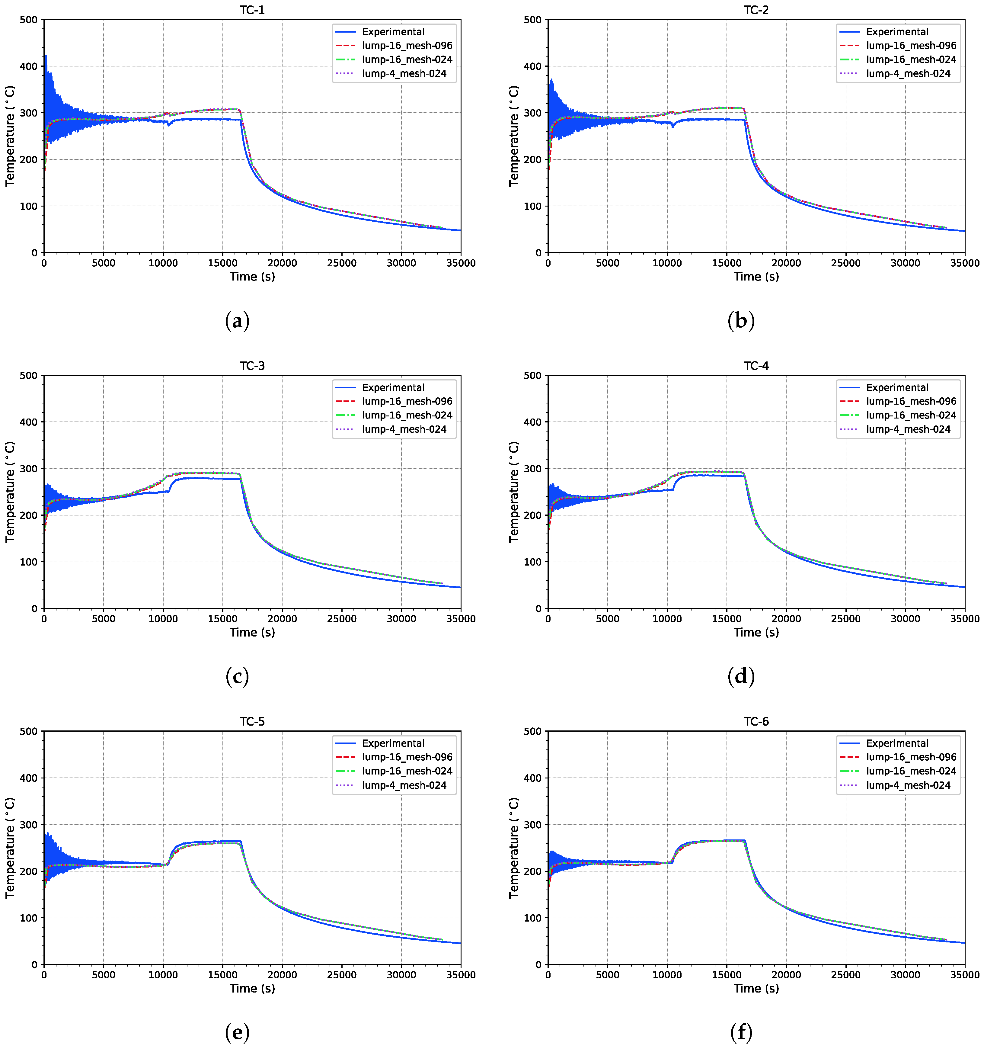
5.1.1. Temperature Evolution

According to Table 3, three heat transfer analyses were conducted for cases #4 to #6. In all instances, the temperature evolution at the six thermocouple positions was plotted (Figure 12). The numerical curves for all cases are nearly identical, indicating that neither the studied lumping strategies nor the mesh sizes significantly affect the thermal behaviour at these points.

When compared to the experimental curves, the macro-level heat transfer analysis is unable to capture the detailed local thermal history at the thermocouples (as expected). However, it effectively captures the average temperature evolution throughout the manufacturing process. Beyond the initial transient period, the agreement between the simulated and measured temperatures is acceptable, with the simulated results closely synchronized with the reference signal.

Different contour-fill plots of the temperature were plotted to evaluate further the impact of layer lumping and mesh size on the temperature output (Figure 13). Minor differences are observed in the bridging zone, a typical hot spot region caused by the overhanging effect. As expected, the smallest lumping case produces slightly higher peak temperatures. However, these differences are negligible and do not significantly impact the EISM predictions.

5.1.2. Distortion

The distortion prediction of the non-symmetrical bridge was evaluated based on the deflection curves along the paths illustrated in Figure 6. The longitudinal distortion was analyzed along the front path prior to the partial removal of supports. Conversely, the vertical distortion of the top surface was assessed along the top path after the supports were removed.

The deflection along the top path provides an indirect means of evaluating the residual stress state of the bridge, particularly the residual stress in the top parallelepiped section. As shown in Figure 14, regardless of the layer lumping strategy, element size, or analysis methodology employed, all cases accurately predict the distortion curve measured experimentally. This indicates that the overall residual stress state at the end of the printing process is well captured by the simulations.

In contrast, the longitudinal deflection exhibits a different behaviour. This deflection represents the distortions that occur during the printing process and is assessed in the as-built state, after the entire domain has cooled. As seen in the experimental deflection curve in Figure 15, the curve consists of two distinct curvatures. The lower curvature corresponds to the rightmost support, while the upper curvature corresponds to the top blocky part of the bridge.

The analysis cases summarized in Table 3 reveal varying distortion behaviours based on modelling aspects. To evaluate the numerical results, two key metrics were computed to quantify the prediction quality of the numerical models relative to the experimental reference curve: the Mean Absolute Percentage Error (MAPE) and the Percent Bias (PBIAS). These metrics, detailed in

Table 4. Summary of MAPE and PBIAS metrics for the front path distortion curves in numerical analysis cases presented in Table 3.

Case	Name	MAPE (%)	PBIAS (%)
#1	lump-4_mesh-024_ISM	50.87	−47.47
#2	lump-16_mesh-024_ISM	56.63	−56.64
#3	lump-16_mesh-096_ISM	56.15	−56.21
#4	lump-4_mesh-024_EISM	10.85	0.01
#5	lump-16_mesh-024_EISM	16.04	−8.95
#6	lump-16_mesh-096_EISM	15.96	−9.09

, provide insights into the accuracy and bias of the models.

When analysing the effect of the modelling methodology, the ISM-based cases (#1–#3) fail to accurately predict the longitudinal deflection curve. High MAPE values (ranging from 50.87% to 56.63%) and significant negative PBIAS (up to −56.64%) indicate large prediction errors and a consistent underestimation of deflection. While ISM can capture the top path deflection, it fails to accurately predict the front path behaviour.

In contrast, the EISM-based cases (#4–#6) demonstrate improved prediction accuracy. The MAPE values are significantly lower, with the best-performing case (#4, lump-4_mesh-024_EISM) achieving a MAPE of 10.85% and a near-zero PBIAS (0.01%). All EISM cases successfully predict the upper profile of the front path deflection. For the lower profile, however, accurate predictions are achieved only when a four-layer lumping strategy is employed.

This explains why cases with a larger lumping size (#5 and #6) exhibit higher MAPE values (approximately 16%) and moderate negative PBIAS (around −9%). These results can be attributed to a singularity effect caused by an abrupt change in stiffness within the structure. Specifically, the rightmost support begins to deflect when layers corresponding to the top blocky part are deposited. During the initial layers, the shrinkage generated by the newly deposited material is counteracted by a progressive increase in stiffness. This phenomenon highlights the importance of using a small lumping size during these initial layers, as it directly affects the curvature of the support leg. This effect often manifests as well-known shrink lines.

Consequently, a small layer lumping size is not necessary for the entire part. Instead, using a smaller lumping size just in the initial layers of the top blocky section would be sufficient to capture the deflection of the support leg reliably.

Interestingly, the variation in mesh size has minimal impact on the distortion curve for a given lumping strategy (see Figure 15b). This finding suggests that employing a one-element-per-layer-thickness strategy is sufficient for accurate predictions, reducing computational complexity without sacrificing accuracy.

Overall, the EISM methodology shows significant improvement over the ISM methodology. In the best case (#4), EISM achieves a 79% reduction in MAPE compared to the best ISM case (#1), where MAPE is reduced from 50.87% to 10.85%. Similarly, EISM improves the PBIAS from −47.47% (#1) to near zero (0.01%, #4), eliminating the systematic underestimation observed in the ISM results. These improvements highlight the enhanced ability of EISM to accurately capture both the location and magnitude of distortions in the bridge structure.

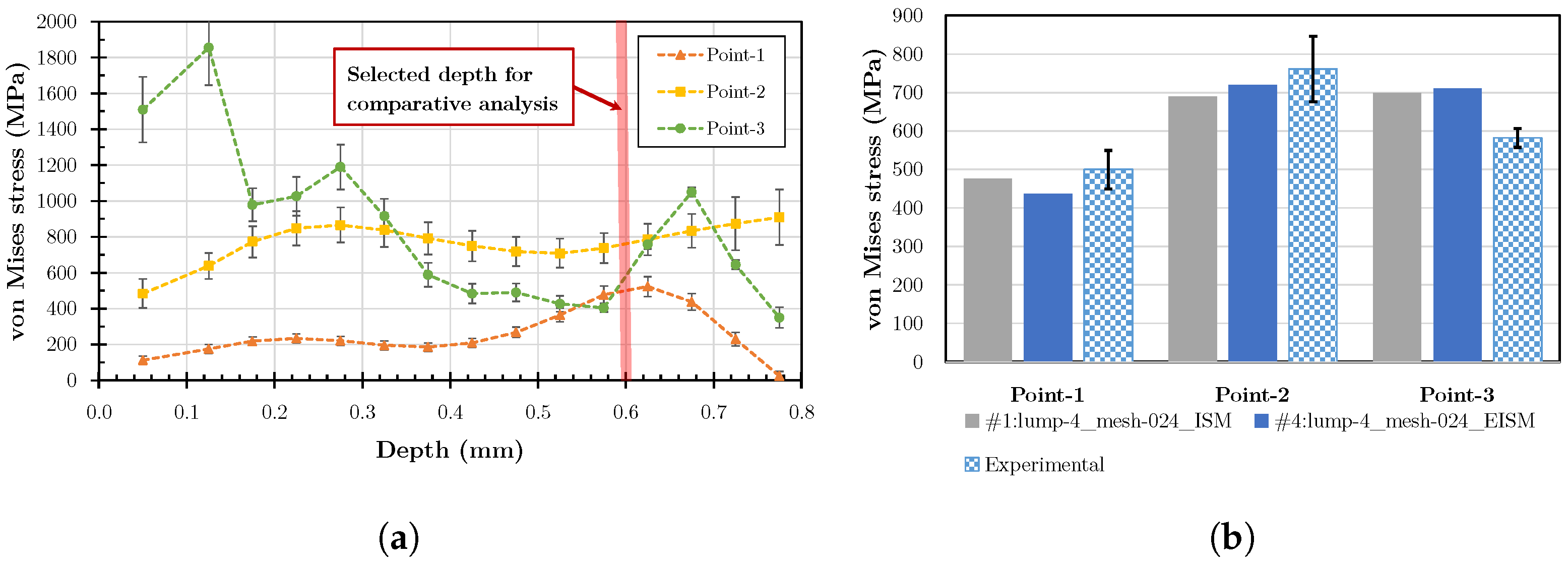
5.1.3. Residual Stress

The von Mises stresses at the points defined in Figure 16 were compared with the experimentally obtained values (see Figure 16a). A depth of $0.6\mathrm{mm}$ was chosen for the comparison to avoid superficial elements and to ensure direct comparison with stress values computed at integration points, without averaging effects.

The numerical cases #1 and #4 were used for the comparison (Figure 16b). Both simulations show good agreement with the hole drilling data, except at point 3, where experimental uncertainties are likely due to near-surface measurements exceeding $70\%$ of the yield stress (ASTM E387-13a).

Overall, the simplified modelling methodologies provide reasonable approximations of the residual stress state, even if not explicitly designed for high-fidelity stress predictions.

5.1.4. Computational Efficiency

To provide a comprehensive evaluation of the proposed methodologies, the computational time for each analysis case was recorded and compared. For the comparison, cases #1, #3, #4, and #6 were selected.

Case #4 was identified as the best-performing case providing the most accurate predictions. However, to establish reference data for computational costs, cases involving the ISM methodology and the 16-layer lumping option (which produces satisfactory results except for the singularity observed at the support leg) were also included.

Table 5. Comparison of computational time for representative bridge analysis cases.

Case	Name	Total CPU Time (h)
		Thermal	Mechanical	Total
#1	Lump-4_Mesh-0.24_ISM	-	5.64	5.64
#3	Lump-16_Mesh-0.96_ISM	-	0.15	0.15
#4	Lump-4_Mesh-0.24_EISM	$5.45$	$7.19$	$12.64$
#6	Lump-16_Mesh-0.96_EISM	$0.13$	$0.17$	$0.30$

summarizes the total CPU time for the selected cases. The results demonstrate that the choice of layer lumping is critical: regardless of the methodology employed, the computational cost increases by approximately 40 times when using smaller lumping sizes.

Regarding the choice of methodology, applying the EISM approximately doubles the computational time required for the ISM due to the need to solve the heat transfer problem alongside the mechanical analysis.

In this context, adaptive layer lumping emerges as a promising option for capturing stiffness changes that occur during the printing process. These stiffness changes can be efficiently identified through pure geometric analysis, as demonstrated in [28]. Furthermore, since smaller layer lumping requires finer mesh resolutions, mesh adaptivity techniques could also be employed to effectively account for this phenomenon.

5.2. SBA

For the SBA, a 16-layer lumping option was selected, resulting in approximately one element per layer thickness. This choice was driven by the large size of the analysis domain and the resulting trade-off in resolution. Under these conditions, it was acknowledged that capturing local distortion magnitudes at shrink-lines with high fidelity might not be feasible. Consequently, two numerical cases were analysed, as summarized in

Table 6. Summary of analysis cases for the SBA.

Case Name	Lumping	Element Characteristic Size (mm)	Methodology
SBA_ISM	16	0.96	ISM
SBA_EISM	16	0.96	EISM

.

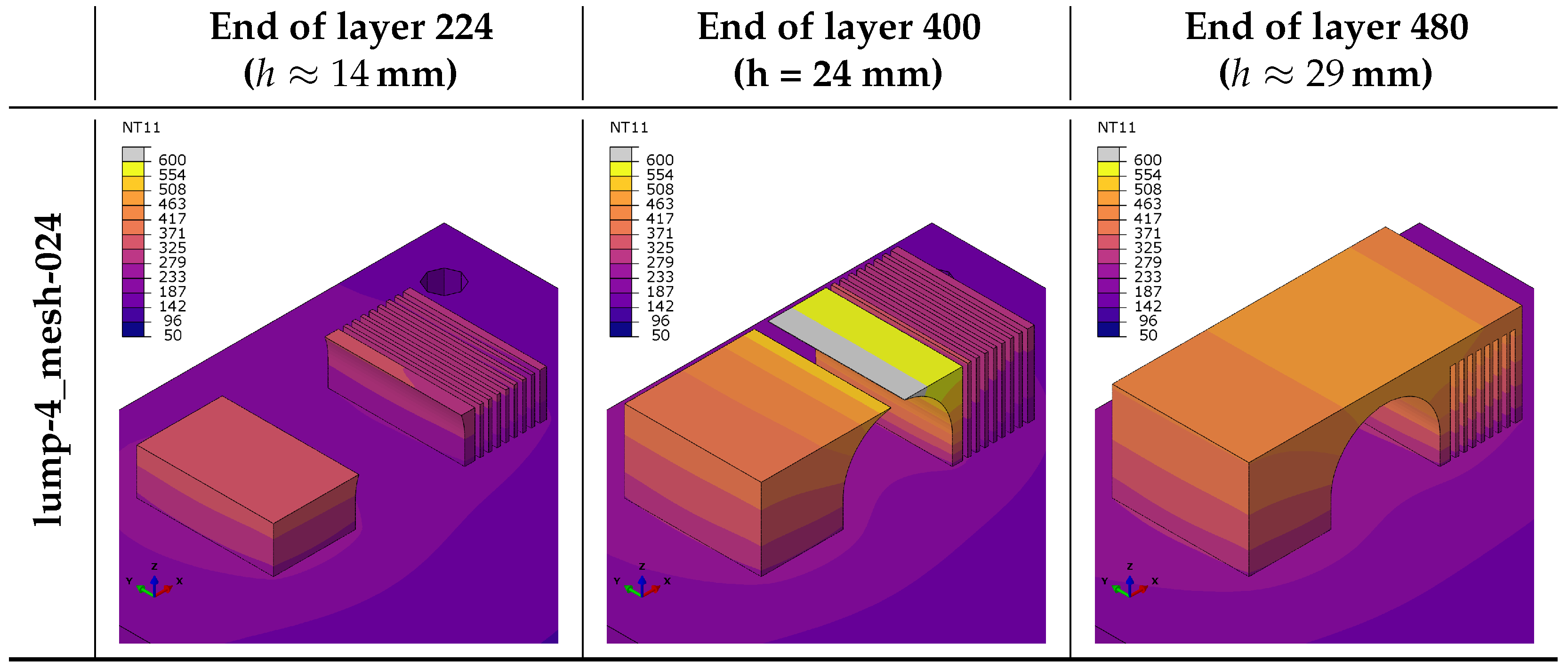
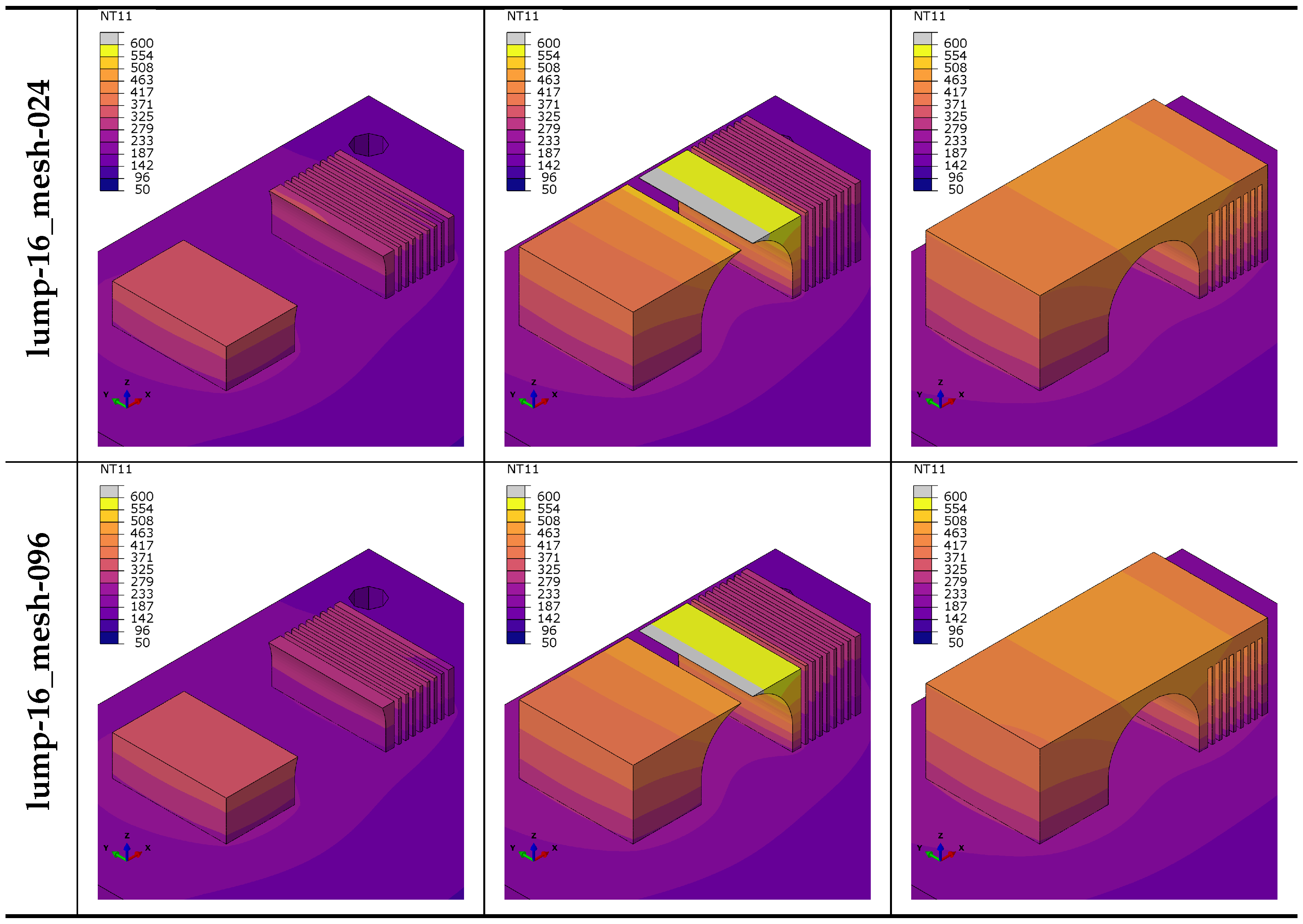
5.2.1. Temperature Evolution

To evaluate the overall behaviour of the part concerning temperature evolution, various instants of the temperature field were plotted, similar to the approach used for the bridge case. In this analysis, relevant time instants were selected to represent different stages of the process, highlighting critical aspects such as hot spots, the effect of part height, and heat dissipation through the surrounding powder (Figure 17).

In this case, the temperature control established at the platform level of the machine loses its effectiveness as the height of the part increases. This is because the greater height reduces the efficiency of heat transfer by conduction, making it more challenging to maintain uniform temperature throughout the part.

5.2.2. Inherent Strain Evolution

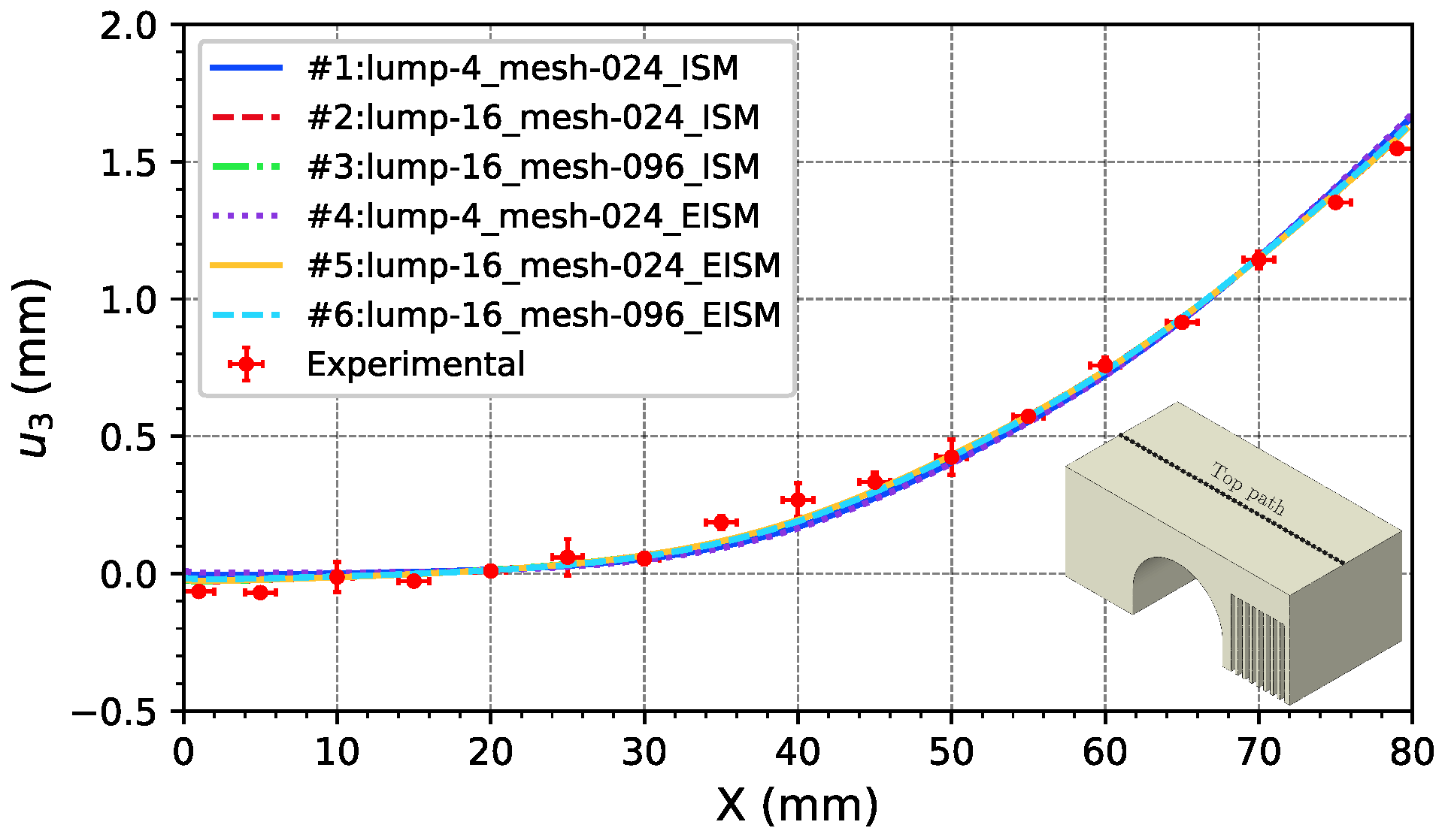
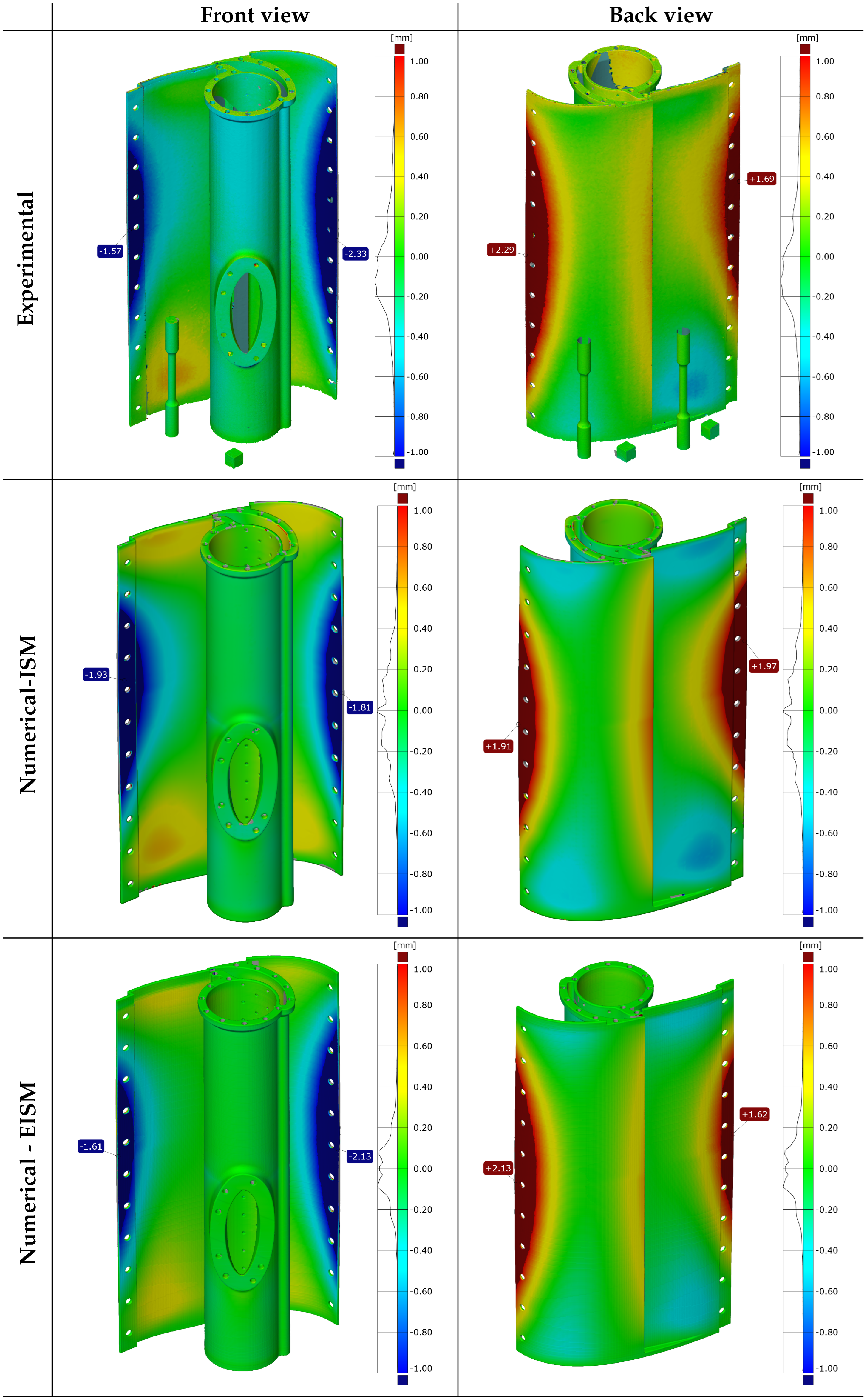
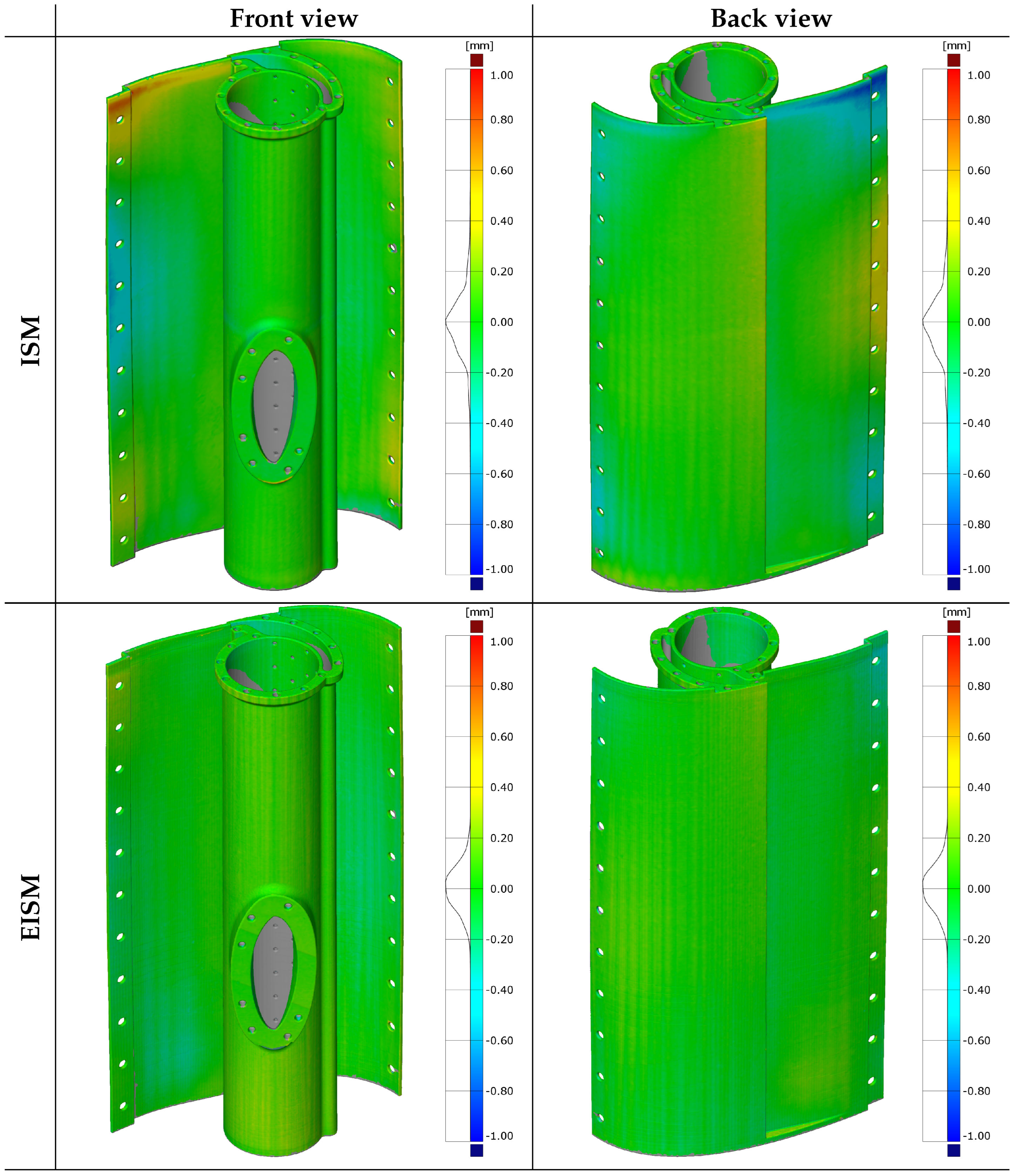
Assessing the evolution of the actually applied inherent strain is crucial to better understand the differences between the ISM and EISM methodologies.

The applied inherent strain at any time is expressed in Equation (12).

To this end, 10 points were selected along the height of the SBA, and the evolution of ${\mathit{\epsilon }}_{xx}^{inh}$ was plotted for both methodologies (see Figure 18a,b).

In the ISM, the full precomputed inherent strain tensor, ${\mathit{\epsilon }}^{inh,0}$, is applied instantaneously upon the activation of each layer, assuming a uniform strain distribution throughout the layer. Conversely, in the EISM, the inherent strain evolves dynamically during the simulation, governed by the temperature history of each point. This evolution is illustrated in Figure 18b for Point 1, as described by Equation (8). The total applied inherent strain at the end of the simulation satisfies ${\mathit{\epsilon }}^{inh}={\mathit{\epsilon }}^{inh,0}$, but the intermediate evolution of ${\mathit{\epsilon }}^{inh}$ is temperature-dependent.

For points near the baseplate, a significant portion of ${\mathit{\epsilon }}^{inh,0}$ is applied predominantly toward the end of the printing process. This is due to prolonged thermal cycles resulting from temperature control in the platform during deposition. In contrast, points near the final layers experience an inherent strain that approaches ${\mathit{\epsilon }}^{inh,0}$ almost instantaneously upon layer activation, closely resembling the behaviour observed in the original ISM.

5.2.3. Distortion

Geometric deviations were calculated by comparing the computed final deformed geometries obtained using both methodologies with the nominal geometry of the SBA. Additionally, geometric deviations were calculated for the experimentally measured deformed shape relative to the nominal geometry. All these deviation contour plots are shown in Figure 19.

When comparing the different deviation contour plots, it can be observed that the ISM method qualitatively captures the overall distortion behaviour of the part; however, some discrepancies are evident. For instance, the locations of the maximum and minimum deviations are not accurately predicted, with these deviations appearing on the opposite wing of the part.

Conversely, the EISM method successfully predicts both the location and magnitude of the deviations. Furthermore, discrepancies in the top section of the part are significantly reduced when using the EISM, demonstrating its superior accuracy in capturing distortion.

A more rigorous way to assess the accuracy of numerical models involves calculating geometric deviations using the experimentally measured deformed shape as a reference. This approach generates deviation contour plots, as represented in Figure 20. If a numerical model were perfectly accurate, no deviations would be observed. The evaluation of numerical models’ prediction accuracy was performed using the metrics of average deviation and its sigma, with the corresponding values summarized in

Table 7. Deviation metrics for numerical models compared to experimental measurement.

Case Name	Average Deviation (mm)	Sigma (mm)
SBA_ISM	−0.01	0.15
SBA_EISM	0.00	0.09

.

The results show that the EISM method (SBA_EISM) achieves an average deviation of 0.00 mm and a lower sigma value of 0.09 mm, indicating both high accuracy and consistency in predicting the experimentally observed deformation. In contrast, the ISM method (SBA_ISM) exhibits a slight bias, with an average deviation of −0.01 mm, and a higher sigma value of 0.15 mm, reflecting greater variability and less reliability in its predictions. Consequently, SBA_EISM demonstrates a 100% improvement in average deviation, effectively eliminating the bias observed in SBA_ISM, and achieves a 40% improvement in sigma, signifying greater consistency in predicting geometric deviations.

5.2.4. Computational Efficiency

Table 8. Comparison of computational time for SBA analysis cases.

Case Name	Total CPU Time (h)
	Thermal	Mechanical	Total
SBA_ISM	-	12.35	12.35
SBA_EISM	8.69	14.19	22.88

summarizes the total CPU time for the selected cases. Like in the bridge case, applying the EISM approximately doubles the computational time due to the need to solve the heat transfer problem alongside the mechanical analysis. Therefore, the accuracy requirement must be well justified. For example, when compensation strategies are to be applied, the EISM is preferable, as it provides refined predictions for predeformation.

6. Conclusions

This work introduced an Enhanced Inherent Strain Method (EISM) for Powder Bed Fusion-Laser Beam (PBF-LB) that incorporates macro-scale temperature histories into the inherent strain formulation. By selectively adjusting the thermal strain component of the precomputed inherent strain tensor according to the evolving thermal field, the EISM more accurately reflects local thermo-mechanical conditions, improving the prediction of distortions and residual stresses compared to the original Inherent Strain Method (ISM).

The methodology was validated against two distinct Ti-6Al-4V geometries: a non-symmetric bridge and a more complex Steady Blowing Actuator (SBA). Comparisons between numerical predictions and experimental measurements of temperature, distortion, and residual stress demonstrated that the EISM offers improved accuracy over the conventional ISM.

The EISM demonstrated notable improvements over the original ISM. For the non-symmetric bridge, Mean Absolute Percentage Error (MAPE) in distortion predictions decreased from 50.87% (ISM) to 10.85% (EISM), representing a 79% improvement. Additionally, EISM eliminated the systematic underestimation observed in ISM, reducing Percent Bias (PBIAS) from −47.47% to 0.01%. For the SBA, EISM reduced the sigma value of geometric deviations compared to experimental measurements from 0.15 mm (ISM) to 0.09 mm, a 40% improvement. EISM also accurately predicted the location and magnitude of maximum distortions, whereas ISM exhibited discrepancies.

A sensitivity analysis revealed that neither the mesh size nor the layer lumping strategy significantly affects the global temperature evolution. However, careful selection of layer lumping and mesh refinement is necessary for layers corresponding to geometry features that represent structural transitions (where abrupt stiffness changes occur, such as those associated with the formation of shrink lines).

Although the EISM approximately doubles computational time compared to the ISM due to the thermal analysis, the added cost remains moderate and justified when higher accuracy is needed. This balance is particularly valuable for industrial applications aiming to reduce trial-and-error procedures and increase confidence in simulation-driven decision-making.

In conclusion, the EISM framework represents a step forward in bridging the gap between simplified original inherent strain-based models and high-fidelity thermo-mechanical simulations.

Future efforts will focus on integrating adaptive mesh and layer lumping strategies as well as exploring automated methods to identify regions requiring finer resolution. Another promising research line could involve improving the thermal model to calculate the temperature history needed in the EISM more efficiently, thereby reducing the computational cost. Such enhancements could further refine the balance between computational efficiency and predictive accuracy. Additionally, extending the EISM approach to other alloys, part geometries, and process parameters will broaden its applicability and increase its relevance in industrial practice.

References

1. Gibson, I.; Rosen, D.; Stucker, B. Additive Manufacturing Technologies; Springer: Berlin/Heidelberg, Germany, 2013; pp. 10–12. [Google Scholar]
2. DebRoy, T.; Wei, H.; Zuback, J.; Mukherjee, T.; Elmer, J.; Milewski, J.; Beese, A.; Wilson-Heid, A.; De, A.; Zhang, W. Additive manufacturing of metallic components—Process, structure and properties. Prog. Mater. Sci. 2018, 92, 112–224. [Google Scholar] [CrossRef]
3. Herzog, D.; Seyda, V.; Wycisk, E.; Emmelmann, C. Additive manufacturing of metals. Acta Mater. 2016, 117, 371–392. [Google Scholar] [CrossRef]
4. Thompson, S.M.; Bian, L.; Shamsaei, N.; Yadollahi, A. An overview of Direct Laser Deposition for additive manufacturing; Part I: Transport phenomena, modeling and diagnostics. Addit. Manuf. 2015, 8, 36–62. [Google Scholar] [CrossRef]
5. Ford, S.; Despeisse, M. Additive manufacturing and sustainability: An exploratory study of the advantages and challenges. J. Clean. Prod. 2016, 137, 1573–1587. [Google Scholar] [CrossRef]
6. Kruth, J.; Froyen, L.; Vaerenbergh, J.V.; Mercelis, P.; Rombouts, M.; Lauwers, B. Selective laser melting of iron-based powder. J. Mater. Process. Technol. 2004, 149, 616–622. [Google Scholar] [CrossRef]
7. Zaeh, M.F.; Branner, G. Investigations on residual stresses and deformations in selective laser melting. Prod. Eng. 2010, 4, 35–45. [Google Scholar] [CrossRef]
8. Bayat, M.; Zinovieva, O.; Ferrari, F.; Ayas, C.; Langelaar, M.; Spangenberg, J.; Salajeghe, R.; Poulios, K.; Mohanty, S.; Sigmund, O.; et al. Holistic computational design within additive manufacturing through topology optimization combined with multiphysics multi-scale materials and process modelling. Prog. Mater. Sci. 2023, 138, 101129. [Google Scholar] [CrossRef]
9. Ueda, Y.; Murakawa, H.; Nakacho, K.; Ma, N. Establishment of computational welding mechanics. Weld. Surf. Rev. 1997, 8, 265–299. [Google Scholar]
10. Mohammadtaheri, H.; Sedaghati, R.; Molavi-Zarandi, M. Inherent strain approach to estimate residual stress and deformation in the laser powder bed fusion process for metal additive manufacturing—A state-of-the-art review. Int. J. Adv. Manuf. Technol. 2022, 122, 2187–2202. [Google Scholar] [CrossRef]
11. Bayat, M.; Dong, W.; Thorborg, J.; To, A.C.; Hattel, J.H. A review of multi-scale and multi-physics simulations of metal additive manufacturing processes with focus on modeling strategies. Addit. Manuf. 2021, 47, 102278. [Google Scholar] [CrossRef]
12. Wang, C.; Tan, X.P.; Tor, S.B.; Lim, C.S. Machine learning in additive manufacturing: State-of-the-art and perspectives. Addit. Manuf. 2020, 36, 101538. [Google Scholar] [CrossRef]
13. Vulimiri, P.S.; Riley, S.; Dugast, F.X.; To, A.C. A mean–variance estimation bidirectional convolutional long short-term memory surrogate model predicting residual stress and model error for laser powder bed fusion. Addit. Manuf. 2025, 97, 104591. [Google Scholar] [CrossRef]
14. Keller, N.; Ploshikhin, V. New Method for Fast Predictions of Residual Stress and Distortion of AM Parts; University of Texas at Austin: Austin, TX, USA, 2014; pp. 1229–1237. [Google Scholar]
15. Setien, I.; Chiumenti, M.; van der Veen, S.; San Sebastian, M.; Garciandía, F.; Echeverría, A. Empirical methodology to determine inherent strains in additive manufacturing. Comput. Math. Appl. 2019, 78, 2282–2295. [Google Scholar] [CrossRef]
16. Setien, I.; Chiumenti, M.; San Sebastian, M.; Moreira, C.A.; Caicedo, M.A. Defining and Optimizing High-Fidelity Models for Accurate Inherent Strain Calculation in Laser Powder Bed Fusion. Metals 2025, 15, 180. [Google Scholar]
17. Chen, Q.; Liang, X.; Hayduke, D.; Liu, J.; Cheng, L.; Oskin, J.; Whitmore, R.; To, A.C. An inherent strain based multiscale modeling framework for simulating part-scale residual deformation for direct metal laser sintering. Addit. Manuf. 2019, 28, 406–418. [Google Scholar] [CrossRef]
18. Dong, W.; Liang, X.; Chen, Q.; Hinnebusch, S.; Zhou, Z.; To, A.C. A new procedure for implementing the modified inherent strain method with improved accuracy in predicting both residual stress and deformation for laser powder bed fusion. Addit. Manuf. 2021, 47, 102345. [Google Scholar] [CrossRef]
19. Dong, W.; Jimenez, X.A.; To, A.C. Temperature-dependent modified inherent strain method for predicting residual stress and distortion of Ti6Al4V walls manufactured by wire-arc directed energy deposition. Addit. Manuf. 2023, 62, 103386. [Google Scholar] [CrossRef]
20. Bugatti, M.; Semeraro, Q. Limitations of the Inherent Strain Method in Simulating Powder Bed Fusion Processes. Addit. Manuf. 2018, 23, 329–346. [Google Scholar] [CrossRef]
21. Du, T.; Yan, P.; Liu, Q.; Dong, L. A process-based inherent strain method for prediction of deformation and residual stress for wire-arc directed energy deposition. Comput. Mech. 2023, 73, 1053–1075. [Google Scholar] [CrossRef]
22. Pourabdollah, P.; Farhang Mehr, F.; Cockcroft, S.; Maijer, D. A new variant of the inherent strain method for the prediction of distortion in powder bed fusion additive manufacturing processes. Int. J. Adv. Manuf. Technol. 2024, 131, 4575–4594. [Google Scholar] [CrossRef]
23. Neiva, E.; Chiumenti, M.; Cervera, M.; Salsi, E.; Piscopo, G.; Badia, S.; Martín, A.F.; Chen, Z.; Lee, C.; Davies, C. Numerical modelling of heat transfer and experimental validation in powder-bed fusion with the virtual domain approximation. Finite Elem. Anal. Des. 2020, 168, 103343. [Google Scholar] [CrossRef]
24. Systèmes, D. Abaqus Analysis User’s Manual. 2024. Available online: https://www.3ds.com/products-services/simulia/support/documentation/ (accessed on 20 December 2024).
25. Moreira, C.A.; Caicedo, M.A.; Cervera, M.; Chiumenti, M.; Baiges, J. An accurate, adaptive and scalable parallel finite element framework for the part-scale thermo-mechanical analysis in metal additive manufacturing processes. Comput. Mech. 2024, 73, 983–1011. [Google Scholar] [CrossRef]
26. Baiges, J.; Chiumenti, M.; Moreira, C.A.; Cervera, M.; Codina, R. An Adaptive Finite Element strategy for the numerical simulation of Additive Manufacturing processes. Addit. Manuf. 2021, 37, 101650. [Google Scholar] [CrossRef]
27. Ganeriwala, R.; Strantza, M.; King, W.; Clausen, B.; Phan, T.; Levine, L.; Brown, D.; Hodge, N. Evaluation of a thermomechanical model for prediction of residualstress during laser powder bed fusion of Ti-6Al-4V. Addit. Manuf. 2019, 27, 489–502. [Google Scholar] [CrossRef]
28. Gladbach, B.; Noe, A.; Rosenhövel, T. Warpage Reduction in Additively Manufactured Parts Based on Thermomechanical Modeling and a Novel Simulation Strategy for Laser Scanning. In New Achievements in Mechanics; Müller, W.H., Noe, A., Ferber, F., Eds.; Springer Nature Switzerland: Cham, Switzerland, 2024; pp. 301–339. [Google Scholar] [CrossRef]
Figure 1. Overview of the EISM methodology, showing the sequential coupling between thermal and mechanical analyses.
Metals 15 00143 g001
Figure 2. CAD model of the non-symmetric bridge geometry (units: mm).
Metals 15 00143 g002
Figure 3. CAD model of the SBA actuator geometry. Bounding box dimensions: 101 × 137 × 306 (mm3).
Metals 15 00143 g003
Figure 4. Laser exposure and recoating time data: (a) non-symmetric bridge and (b) SBA actuator.
Metals 15 00143 g004
Figure 5. Schematic of thermocouple (TC) locations within the baseplate. Each thermocouple is labelled as TC-x, indicating its specific position. The detail view provides a detailed representation of the thermocouple arrangement, highlighting their placement within machined blind holes to measure temperatures as close as possible to the top surface of the baseplate.
Metals 15 00143 g005
Figure 6. Schematic showing front and top paths where distortion measurements were taken for the non-symmetric bridge.
Metals 15 00143 g006
Figure 7. State of the bridge geometry before and after partial cutting to release residual stress: (a) state of the bridge before the cut and (b) state of the bridge after the cut. The detailed view highlights the cut zone, where the bridge was partially released from the baseplate.
Metals 15 00143 g007
Figure 8. Locations of the three measurement points for residual stress analysis on the non-symmetric bridge.
Metals 15 00143 g008
Figure 9. Geometrical model and FE mesh of the non-symmetric bridge, including the baseplate: (a) geometrical model and (b) 3D FE mesh.
Metals 15 00143 g009
Figure 10. Geometrical model and FE mesh of the SBA with the baseplate: (a) geometrical model and (b) 3D FE mesh.
Metals 15 00143 g010
Figure 11. Comparison of non-symmetric bridge meshes with different characteristic element sizes: (a) fine mesh with a characteristic element size of 0.24 mm and (b) coarser mesh with a characteristic element size of 0.96 mm .
Metals 15 00143 g011
Figure 12. Comparison between numerically predicted and experimentally recorded temperature histories at the thermocouple locations: (a) TC-1, (b) TC-2, (c) TC-3, (d) TC-4, (e) TC-5, and (f) TC-6.
Metals 15 00143 g012
Figure 13. Evolution of the temperature field of the non-symmetric bridge during the deposition process.
Metals 15 00143 g013aMetals 15 00143 g013b
Figure 14. Top path distortion comparison between numerical and experimental data.
Metals 15 00143 g014
Figure 15. Front path distortion for the non-symmetric bridge, illustrating the influence of (a) layer lumping, (b) mesh size, and (c) methodology.
Metals 15 00143 g015
Figure 16. von Mises residual stress measurements and comparison at three points. (a) Experimentally measured evolution through the depth and (b) comparison with numerical results.
Metals 15 00143 g016
Figure 17. Temperature contour plots of the SBA actuator at different printing stages: (a) h 30 mm , (b) h 78 mm , (c) h 164 mm , (d) h 230 mm , (e) h 298 mm , and (f) h 305 mm .
Metals 15 00143 g017
Figure 18. Evolution of ε x x i n h at different points along the height of the SBA part: (a) ISM methodology and (b) EISM methodology.
Metals 15 00143 g018
Figure 19. Deviation contour plots of the SBA, calculated relative to the nominal geometry. Results are shown for experimental data (top row), numerical-ISM (middle row), and numerical-EISM (bottom row), with front and back views.
Metals 15 00143 g019
Figure 20. Deviation contour plots of the SBA, calculated relative to the experimentally measured deformed geometry. Results are shown for ISM (top row) and EISM (bottom row), with front and back views.
Metals 15 00143 g020