1. Introduction
Perforated stainless steel is widely used for industrial and medical purposes. Key areas of use include filtration, separation, drying, as well as their utilization as components in various technical devices. In medicine, perforated stainless steel is used, for example, for bone regeneration [
1]. The mechanical properties of the material, such as the effective elastic modulus, significantly influence the durability of implants and their adaptation to the applied load [
2,
3,
4]. The presence of perforations alters the material’s structure, reduces its load-bearing capacity, and affects the stress distribution within the material [
2]. To ensure an effective and biomechanically compatible implant design, it is crucial to understand the dependence of the effective elastic modulus on the relative perforation area in cylindrical structures. Measurements on perforated structures allow for the evaluation of their mechanical properties for specific applications, such as the manufacture of medical implants [
3]. Recent work on thin, porous layers shows that standardized physical and mechanical assessment combining tensile response with light-permeability and breathing-resistance tests (EN 149 [
5]) is decisive for discriminating performance-critical behavior in architected sheets [
6]. One of the most significant challenges in implantology is the discrepancy between the elastic modulus of the implant and that of natural bone, which can lead to stress shielding. This phenomenon promotes bone resorption and may result in implant loosening [
4,
7,
8,
9,
10]. Perforated materials are used in implants to reduce the weight of structures, ensure the circulation of bodily fluids, and promote tissue integration. Due to their high biocompatibility, they help to improve the healing process [
7,
11,
12]. In medicine, perforated cylindrical elements are used as implants for the fixation and support of bone structures.
The use of cylindrical thin-walled structures reduces the implant’s mass, thereby decreasing the load on surrounding tissues. The perforated structure facilitates customization to the patient, as the implant features an adjustable height. The open architecture of the titanium mesh promotes bone ingrowth and optimizes osseointegration. Rings at the ends of the mesh ensure correct spinal alignment after rehabilitation [
13]. In previous studies on flat perforated specimens, the influence of perforation on their mechanical properties and load-bearing capacity was analyzed [
2]. The impact of geometric parameters and mechanical properties of perforated materials on their load-bearing capacity was investigated, with particular attention paid to stress distribution within the material, which significantly affects its strength and durability [
2,
14]. The relative perforation area is an important variable influencing the elastic response of cylindrical shells in this investigation since geometric configuration can independently regulate effective stiffness [
15]. Numerical analyses indicate that material curvature and plastic properties influence stress, while mechanical testing of porous titanium alloys reveals structural changes under load [
16]. Methodology with numerical modeling and inverse analysis, was used to determine the elastic modulus of electrospun nanofibrous mats by correlating their vibrational response with finite element simulations [
15,
17]. Studies on flat specimens have revealed that the elastic modulus decreases with an increasing perforation area; however, there is currently a lack of data to predict changes in the effective elastic modulus in perforated cylindrical implants [
2,
18].
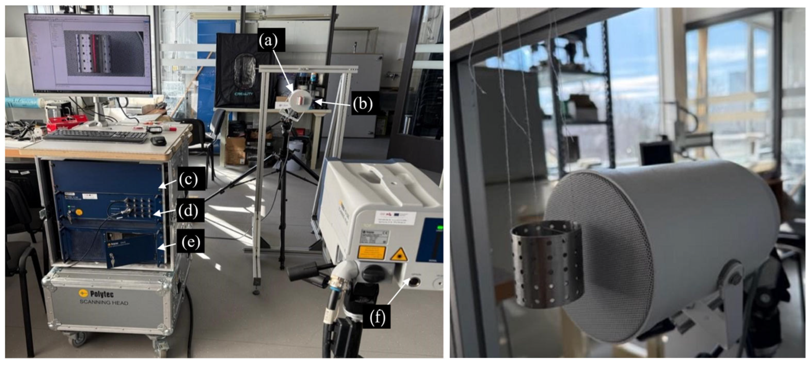
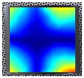
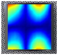
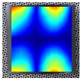
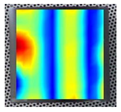
This research analyzes the dependence of the effective elastic modulus on the relative perforation area in perforated, cylindrical stainless-steel specimens. The determination of their frequency characteristics and the visualization of the corresponding mode shapes were performed using a non-contact “Polytec PSV 500 3D” (Polytec GmbH, Waldbronn, Germany) laser vibrometer. The research was conducted at the Institute of High-Performance Materials and Structures of Riga Technical University. Finite element analysis was subsequently used to determine the effective elastic modulus of the stainless-steel material for these specimens [
18,
19]. Numerical analysis was previously developed for the determination of the elastic properties of composite materials [
20] and was adopted for perforated steel cylinders. The manufacturing of cylindrical perforated implants enables the rehabilitation of tubular bone injuries. Although cylindrical implants are typically made from titanium, stainless steel is still used for temporary structures [
21,
22,
23,
24,
25]. Due to its comparable properties and wide availability, stainless steel is also an economically advantageous alternative [
26,
27]. Stainless steel 304 was selected due to its established biocompatibility, corrosion resistance, and mechanical stability, which make it suitable for biomedical applications. In addition, stainless steel can serve as an alternative material in cases of allergy or intolerance to titanium alloys, offering a clinically viable option for implant design. No studies have been conducted to analyze the dependence of the effective elastic modulus on the relative perforation area for perforated stainless-steel cylinders, this work is aimed at uncovering this behavior.
2. Materials and Methods
2.5. Numerical Experiment on Elastic Properties Determination of Perforated Stainless Steel 304 Cylindrical Specimens
To determine the numerical model’s resonance frequencies and corresponding resonant mode shapes, a modal analysis using the Lanczos algorithm is employed. The Lanczos algorithm is a computational method that utilizes only matrix multiplication with long, narrow matrices [
33]. In the experiment, the geometric parameters of the outer surface shape and dimensions-obtained from 3D-scanned models were used to create the numerical models. The thickness of the specimen material (1 mm) was assigned to the outer surface geometry of the models obtained by the scanner, so that the numerical model would correspond to the physical specimen. The density of these models corresponds not to the theoretical density of stainless steel, but to the equivalent density of each physical specimen. The equivalent density
ρ of each specimen was calculated by weighing each specimen and determining its geometric dimensions, using Equation (4).
In Equation (4),
ρ is the equivalent density of the specimen,
m is the mass of the specimen,
V is the volume of the specimen,
l is the length of the specimen,
w is the width of the specimen, and
h is the thickness of the specimen material. The specimen dimensions, masses, and calculated equivalent densities are summarized in
Table 2.
When creating the numerical models, the scanned surfaces of the specimens without perforations were used, as this allows for the determination of the specimen’s resonance frequencies. In the case of modeling perforated specimens, the resulting values would characterize the elastic properties of stainless steel, which are already known.
Based on the results shown in
Table 3, an 8 × 24 mesh was selected for the model of specimen 1, as increasing the number of elements from 7 × 21 to 8 × 24 elements did not significantly alter the calculated frequencies. The resonance frequency values changed within a range of 0.5%. This indicates a stable model and that the resonance frequencies of the finite element models were determined with 0.5% accuracy.
The resonance frequencies of the three-dimensional models were calculated using the finite element method. The finite element analysis was performed in ANSYS Mechanical APDL. The three-dimensional geometries of the scanned specimens were imported in IGES format and verified for dimensional accuracy using keypoint distance queries to confirm the correct scale in meters. Prior to meshing, the geometry was simplified by removing unnecessary solid regions, leaving only the thin shell surface representing the cylindrical wall of each specimen. The SHELL181 element type was selected as it provides reliable performance for thin-walled, curved structures under modal analysis conditions. Material properties, namely the elastic modulus, Poisson’s ratio, and effective density were defined for each simulation according to the experimental plan, using measured specimen mass and geometric parameters to calculate equivalent density. The shell thickness was assigned as 1 mm, corresponding to the physical specimen. Mesh density was determined based on the convergence analysis described earlier; a uniform mapped mesh was generated to achieve stable resonance frequency results. The modal analysis was configured using the Block Lanczos solver with 30 natural modes requested to ensure that the frequency range covered all experimentally observed resonances. After solving, the obtained eigenfrequencies and mode shapes were compared with experimental data to verify numerical accuracy. The APDL environment was chosen over Workbench because it enables direct command-level control, parameter scripting, and efficient batch processing of multiple models, which is essential for full factorial simulation runs and subsequent parameter identification. When a case is reached where the sequences of resonance frequencies from the physical experiments and the numerical calculations coincide, it can be concluded that the properties corresponding to the elastic properties of the physical specimens have been found. The solution to the problem involved analyzing the coincidence of the first fifteen resonance frequencies. The correct identification of the resonance sequence was confirmed by comparing the mode shapes from both the experiments and the numerical calculations. This comparison allowed for a double-check and ensured the correct identification of the elastic properties. Furthermore, solving the inverse problem in conjunction with the numerical method provides the opportunity to conduct research in a non-invasive environment, preserving the specimens for future experiments, which cannot be said for mechanical tests.
The application of the inverse problem facilitated the achievement of the stated research objective, thereby helping to reveal the effective elastic properties of the studied specimens.
2.6. Approximation of Experimental Data Using the Least-Squares Method
Approximation allows for obtaining a general description of a function that better fits noisy or incomplete data. Approximation methods are applied in physics and engineering to characterize complex processes and experimentally obtained data that cannot be described by simple functions. The approximation of the numerically obtained resonance frequencies was carried out using the least-squares method implemented in Python version 3.12.7 (Visual Studio Code version 1.105.1).
The least-squares method is one of the most popular and widely used approaches for performing approximation. Its fundamental principle is to find a function that minimizes the error between the initial data and the approximated function [
34]. More precisely, the least squares method optimizes the function to reduce the squared deviations between the observed data and the approximated value shown in Equation (5).
S is the error function that is minimized, n is several specific values, yi is an experimentally determined values and g(xi) is approximate value.
The least-squares method was used to formulate a regression equation expressed as a second-order polynomial. Approximation with a polynomial is employed to mathematically describe the relationship between variables using a polynomial function that provides the best possible fit to the experimental data. A second-order polynomial is one of the most used regression models, as it can represent both linear and nonlinear relationships between variables [
35]. In its general form, a second-order polynomial is expressed as follows, shown in Equation (6).
y is the dependent variable (result),
x is the independent variable (input parameters), and
a0,
a1, and
a2 are polynomial coefficients. Such a regression equation is applied in situations where the relationship between input and output data is not linear and more accurate data modeling is required than in the case of linear regression. The least-squares method is used to determine the second-order polynomial so that the function fits the experimental data as closely as possible. The fundamental principle of this method is to minimize the error between the experimentally obtained values and the values of the approximation function. Mathematically, this is described by Equation (7).
where
yk is the target value,
xk is the independent variable value,
m is the number of experimental data points, and
S is the function that calculates the total square error.
The formulation of the approximating polynomial involves several steps. First, experimental data to be approximated are obtained. Subsequently, a system of equations is established, corresponding to a solution by the least-squares method. This system of equations is solved, resulting in the calculation of the regression equation coefficients [
35]. As a result, a regression equation expressed as a second-order polynomial with appropriately determined coefficients is obtained.
After calculating the coefficients of the regression equation, it is possible to construct a response surface. A response surface is a mathematical modeling method used to visually analyze how different factors influence the outcome [
36]. Numerical experiments were conducted based on experimental design. Following the application of the finite element method, the numerically obtained results were approximated using the least-squares method. In the numerical experiment, sequences of resonance frequencies were obtained for various combinations of elastic parameters. For each combination, the sequence of the first 15 resonance frequencies was determined, the agreement of which was confirmed by visualizing the mode shapes and comparing them with the resonance sequences obtained from physical experiments. A second-order regression equation, shown in Equation (8), was applied to approximate the results of the numerical experiment [
18,
19].
fi is the i-th order resonance frequency, E is the modulus of elasticity, v is Poisson’s ratio, and b0i, b1i, b2, b12i, b11i, and b22i are the coefficients of the second-order regression function.
3. Results
The determination of the dependence of the effective elastic modulus on the relative perforation area begins with obtaining the resonance frequency sequence and corresponding mode shapes for each physical specimen.
Table 4 summarizes the results of the physical experiments and numerical experiment for specimen Nr. 1.
As can be seen from
Table 4, specimen Nr. 1 exhibits various characteristic mode shapes, which change depending on the vibration order. The resonance frequencies gradually increase, starting from 1116 Hz (physical experiment) and 1113 Hz (numerical experiment), up to 10,332 Hz (physical experiment) and 10,314 Hz (numerical experiment).
Prior to performing the finite element analysis, a convergence check was conducted for each model.
Table 4 shows an example of the convergence check for a model with a diameter of 47.7 mm, a height of 50 mm, and a thickness of 1 mm. For all models during the check, a density of 7850 kg/m
3 was assumed, corresponding to the density of the studied material. The evaluation utilized the first 15 determined resonance frequency values, analyzing the influence of mesh density within the range of 1 × 3 to 22 × 66 finite element distribution.
Figure 8 demonstrates the stability of the convergence result for the 3rd, 7th, and 14th order resonance frequencies of specimen Nr. 1.
As can be seen from
Figure 7, the resonance frequencies converge depending on the number of finite elements used. Thus, the selected mesh density for each model does not affect the accuracy of the numerical calculations, ensuring reliable modeling results. This analysis allowed for the selection of the most appropriate mesh density for each model, maintaining high computational accuracy and avoiding unnecessary consumption of computational resources. It can also be observed that higher-order resonance frequencies (such as the 14th resonance frequency) are more sensitive to mesh refinement and require a larger number of finite elements to achieve stabilization. In contrast, lower-order modes converge faster, resulting in smaller deviations and reduced numerical error even with coarser meshes. After the convergence check of the final models, the finite element method was performed, and the obtained results were approximated using a second-order regression function.
A separate second-order regression function was fitted for each resonance frequency, which allowed for detailed modeling of the dependence of these frequencies on the elastic modulus
E and Poisson’s ratio. The regression coefficients were determined using the least-squares method and are listed in
Table 5.
Regression coefficients provide the ability to evaluate the influence of each parameter on the resonance frequency. The regression function coefficients b1i and b2 characterize the direct dependence on E and v, while the coefficients b12i, b11i, and b22i reflect the mutual interaction of the parameters. Based on the obtained coefficients, response surfaces were created. Surfaces visualize the variation in each resonance frequency depending on the selected material parameters. Response surfaces were used to perform approximation for the entire set of experiments, thereby ensuring that no errors were introduced during the input of the numerical experimental data.
To verify the quality of the approximation, a comparison was made between the numerical and approximated frequencies. The average and maximum relative errors, as well as the coefficients of determination, were calculated for each of the 15 resonance frequency series. The average relative error was calculated using Equation (10).
MRPE is a mean relative percentage error, N is a number of resonance frequencies used in the identification procedure, yi is a resonance frequency value obtained from the numerical experiment, and ŷi is an approximated resonance frequency value.
Using the built-in “max” function in Microsoft Excel, the maximum relative error value was determined for each frequency. After calculating the average and maximum relative error values, the coefficient of determination
R2 was determined for each frequency using Equation (11).
R2 is a coefficient of determination, ŷi is a resonance frequency value obtained from the numerical experiment, is an approximated resonance frequency value, and ȳ is a mean value of the approximated frequencies.
Below is an example of the coefficient of determination calculation for the 6th resonance frequency of sample Nr. 1. To simplify the calculation, the numerator of the expression was computed first, followed by the mean value of the approximated resonance frequency for the given order frequency, and then the denominator.
Table 6 presents the average and maximum relative errors, as well as the coefficient of determination values, for all 15 frequency series of sample Nr. 1.
The values of the effective elastic modulus and the effective shear modulus were determined for each sample and are summarized in
Table 7. The experimentally and numerically obtained resonance frequencies and elastic property values for all samples are also presented.
After processing the results and determining the optimal effective elastic modulus values for each sample, it became possible to evaluate the dependence of the effective elastic modulus of the perforated cylinder on the relative perforation area.
4. Discussion
The main goal of this research is to investigate the dependence of the effective elastic modulus of a perforated stainless-steel cylinder on the relative perforation area. Microsoft Excel software was used to process the results of the dependence of the effective elastic modulus values of cylindrical specimens on the relative perforation area. The software was utilized to compile results in
Table 8 from the obtained data and to create a graph of the studied dependencies (
Figure 8 and
Figure 9). The research determined the effective elastic modulus values of a grade 304 stainless-steel cylinder, as well as obtained the effective shear modulus values for cylinders with a relative perforation area ranging from 0% to 50.24%. The experimentally obtained data are presented in
Table 8.
The
Table 8 specifies the sample number, perforation diameter, relative perforation area, and the values of the effective elastic and shear moduli. The data from the
Table 8 shows that an increase in the relative perforation area from 0% to 50.24% causes a decrease in the elastic modulus from 184.76 GPa to 50.69 GPa, indicating a deterioration in the stiffness properties of the material studied. This reduction can be explained by the fact that as the relative perforation area increases, the effective cross-sectional area of the material capable of bearing the load decreases, leading to elevated stress concentrations around the perforations.
The data presented in the table also indicate a similar trend for the effective shear modulus. As the relative perforation area increases, the effective shear modulus decreases from 67.34 GPa to 21.12 GPa. This parameter is used to determine the material’s ability to resist shear deformation. The shear modulus is another important factor considered during implant manufacturing, as it indicates the mechanical strength and stability of the material used.
Based on the obtained results, it can be concluded that an increase in the relative perforation area leads to a deterioration of the elastic properties in stainless steel, while simultaneously making it mechanically closer to the properties of human bone.
Figure 9 illustrates the dependence of the effective elastic modulus on the relative perforation area. The graph demonstrates that an increase in the relative perforation area leads to a reduction in the effective elastic modulus. The elastic modulus describes a material’s ability to resist elastic deformation. For grade 304 stainless steel, the elastic modulus value without perforations typically ranges from 190 GPa to 203 GPa.
In the studied cylinder without perforations, the effective elastic modulus was 184.76 GPa. Introducing perforations with a diameter of 3 mm, resulting in a relative perforation area of 7.07%, reduced the elastic modulus to 160.47 GPa. Increasing the relative perforation area to 12.56% further decreased the effective elastic modulus to 138.25 GPa. At a relative perforation area of 23.75%, the effective elastic modulus reached 112.02 GPa. When the relative perforation area increased to 50.24%, the effective elastic modulus decreased to 50.69 GPa. The reduction of the relative perforation area from 0% to 50.24% resulted in a sharp decline in the effective elastic modulus. The numerical decrease was 134 GPa, representing a percentage difference of 73%. The graph shows that increasing the relative perforation area from 0% to 20% reduces the effective elastic modulus by 60 GPa, resulting in a relative difference of 34%. Further increasing the perforation area from 20% to 40% reduces the effective elastic modulus by approximately 45 GPa, corresponding to a relative difference of 37.5%. The increase in perforation diameter and the reduction in ligament width between holes lead to a decrease in the effective elastic modulus, as the reduced load-bearing cross-sectional area and stress concentration around the perforation edges diminish the material’s overall stiffness. This tendency agrees well with earlier research findings, which also demonstrated that increasing perforation size or density leads to a reduction in the effective stiffness of the structure [
30].
Based on this analysis, it can be concluded that the effective elastic modulus decreases linearly and uniformly. The graph reveals a linear decreasing trend, described by a regression function with a very high coefficient of determination (R
2 = 0.9905). This high R
2 value indicates that the chosen regression curve accurately reflects the observed relationship between the effective elastic modulus and the relative perforation area. The studied dependence can be mathematically described by Equation (12).
E is an effective elastic modulus and RP is a relative perforation area. This regression function allows for the prediction of elastic modulus values even beyond the experimentally obtained data points within a defined range. The function also indicates that as the perforation area increases, the effective elastic modulus decreases almost uniformly.
The elastic modulus values of human bone fall within the range of 10 GPa to 30 GPa, which is highlighted in orange in
Figure 8. Based on the results obtained in this research, the closest approximation to human bone is sample Nr. 5, with an effective elastic modulus of 50.69 GPa, as its value is the lowest compared to the other samples. Despite having the smallest difference in elastic modulus, there remains a high risk of bone resorption, which could lead to implant loosening. Therefore, to achieve even greater similarity to the elastic properties of human bone, it would be necessary to investigate the effective elastic modulus values of perforated stainless-steel cylinders with a relative perforation area exceeding 50%. In the author’s opinion, it would also be useful to study the influence of the perforated cylinder’s diameter on the effective elastic modulus value, as there may be a correlation that causes this value to increase or decrease.
Within the framework of the research, the values of the effective shear modulus were also determined for each sample, as indicated in
Figure 10. The shear modulus characterizes the material’s ability to resist shear deformation. Similarly to the elastic modulus, a pronounced decrease is observed for the effective shear modulus. For the sample without perforations, the obtained effective shear modulus value was 67.34 GPa, whereas for the sample with the largest relative perforation area, this value decreased to 21.12 GPa. Such a reduction in the effective shear modulus significantly impacts the material’s ability to resist shear deformation, which is important to consider when developing biomechanical implants.
The research results also indicate a decrease in the sequence of resonance frequencies with an increase in the relative perforation area. The first resonance frequency of sample Nr. 1 is 1116 Hz, and the highest is 10,332 Hz, while for sample Nr. 5, the first frequency is already 827 Hz and the last is 7889 Hz. This confirms that, alongside the deterioration of the material’s effective cross-section and stiffness, the resonance frequencies across the system also decrease. The presence of larger or more closely spaced perforations lowers the effective shear modulus due to the reduced number of shear load paths and the concentration of local shear strains within the thin ligaments between perforations.
The average error between the experimentally and numerically determined resonance frequencies increases with the perforation area, mainly due to higher stress concentration, reaching a maximum average error of 1.01% at a 50.24% relative perforation area. According to the data provided in the table, the maximum relative error between experimentally and numerically determined frequencies reached 1.97%. These errors are associated with the approximation process, which utilizes the least-squares method and error functional minimization. It should be noted that numerical frequency values were obtained using the finite element method. The precision of the numerical model played a significant role in this process, as mentioned earlier-the 3D scanner ensured geometric model accuracy up to 1.5%. The accuracy of the numerical frequencies could also be influenced by the discretization of the numerical model into finite elements, whose mesh convergence was selected with an accuracy of up to 0.5%. Therefore, in the author’s opinion, the effective elastic modulus values were determined with a maximum relative error between the experimental and numerical resonance frequencies reached 1.97%, which may result from slight inaccuracies in boundary conditions and geometric simplifications in the numerical model, but the obtained numerical frequency values could also be influenced by other applied methods. The total result error could reach up to 5%, mainly due to combined uncertainties in material properties, geometry, and experimental measurements.
Recent advances in materials science have shown that geometric structuring can be used not only to adjust stiffness but also to induce unusual deformation characteristics, such as a negative Poisson’s ratio (auxetic behavior) [
43,
44]. Perforation-based design approaches therefore provide a versatile route to tailoring mechanical response, combining light weight with adjustable elastic properties. This concept is of particular interest for biomedical implants, where local compliance and energy absorption are critical.
The results of this study demonstrate that the geometric configuration of perforations significantly influences the elastic and shear properties of cylindrical structures. This geometry-driven behavior aligns with the concept of mesoscale architecture, where structural design is used to control macroscopic mechanical response. Recent research on mechanical metamaterials confirms that periodic geometric modifications can enable tunable stiffness and functional adaptability [
45,
46]. The present work thus provides a practical example of geometry-based optimization of mechanical performance and contributes to the broader understanding of architectured material design. These findings may also support future developments in biomedical and lightweight engineering applications, where mechanical efficiency and functionality are equally important [
43].
5. Conclusions
This research successfully applied a non-destructive method for determining the effective elastic modulus of perforated 304 stainless-steel cylinders. The method was based on determining the resonance frequencies of physical specimens using a non-contact vibrometer and solving an inverse problem for numerical models utilizing the finite element method, approximation via the least-squares method, second-order regression functions, as well as the formulation and minimization of an error functional.
The results show that as the relative perforation area increases, the elastic properties of perforated 304 stainless-steel cylinders significantly decrease. With an increase in the relative perforation area from 0% to 50.24%, the effective elastic modulus decreased from 184.76 GPa to 50.69 GPa.
A high degree of agreement was observed between the experimentally and numerically obtained resonance frequency values. The average relative error for all specimens did not exceed 1.01%, while the maximum relative error was less than 2%.
An increase in the relative perforation area leads to a decrease in resonance frequencies—the smaller the perforation area, the higher the frequencies, whereas as the perforation area increases, the frequency values gradually decrease. A larger perforation volume lowers resonance frequencies by reducing stiffness.
The decrease in the effective elastic modulus values affects the material’s mechanical properties. For future studies, it is recommended to also investigate the strength and fatigue properties of perforated 304 stainless-steel cylinders to more thoroughly identify the factors causing the deterioration of the material’s mechanical properties with increasing relative perforation area.
To identify the deeper causes of the perforation-induced reduction in elastic properties, it is recommended to analyze internal changes in the material at the microscopic level. This investigation will help determine whether and how perforations cause local changes in the material’s structure that affect its mechanical behavior.
In future studies we recommend defining optimal parameters for practical applications, especially in medical implant design. This would allow defining optimal parameters for practical applications, particularly in the development of medical implants. Also, future studies should consider a more detailed numerical representation of the perforation geometry to better capture local stress effects and improve the accuracy of elastic property evaluation.
Therefore, future studies should focus on a more detailed analysis of these geometric factors, especially on perforation areas lower than 50%, to establish predictive relationships between perforation geometry and the effective elastic properties of such structures.
Author Contributions
Conceptualization, P.A., A.S. (Anastasija Sirotkina), M.O. and V.M.; methodology, A.S. (Anastasija Sirotkina), V.M. and P.A.; software, P.A. and A.S. (Anastasija Sirotkina); investigation, A.S. (Anastasija Sirotkina), V.M., P.A. and M.O.; data curation, A.S. (Anastasija Sirotkina), V.M., P.A. and M.O.; writing—original draft preparation, A.S. (Anastasija Sirotkina), M.O., visualization, A.S. (Anastasija Sirotkina), P.A. and M.O.; project administration, V.M., M.O., A.S. (Anastasija Sirotkina), I.L. and A.S. (Andris Skromulis). writing—review and editing, M.O., A.S. (Anastasija Sirotkina), V.M., P.A. and I.L. All authors have read and agreed to the published version of the manuscript.
Funding
The study was supported by research and development grant No RTU-PA-2024/1-0091 under the EU Recovery and Resilience Facility funded project No. 5.2.1.1.i.0/2/24/I/CFLA/003 “Implementation of consolidation and management changes at Riga Technical University, Liepaja University, Rezekne Academy of Technology, Latvian Maritime Academy and Liepaja Maritime College for the progress towards excellence in higher education, science, and innovation”.
Data Availability Statement
The data presented in this study are available on request from the corresponding author. The data are not publicly available due to privacy restrictions.
Conflicts of Interest
The authors declare no conflicts of interest.
References
- Hunt, P.; Unterhauser, F.N.; Strobel, M.J.; Weiler, A. Development of a perforated biodegradable interference screw. Arthroscopy 2005, 21, 258–265. [Google Scholar] [CrossRef]
- Ahmed, M.S. Numerical Analysis of the Perforated Steel Sheets Under Uni-Axial Tensile Force. Metals 2019, 9, 632. [Google Scholar] [CrossRef]
- Chentsov, A.V.; Goldstein, R.V.; Mokryakov, V.V.; Andreev, A.O.; Petrovskii, V.N.; Gleser, A.M.; Libman, M.A. Experimental measurements of the effective elastic modulus of steel specimens containing lattices of circular holes. In Proceedings of the 17th International Conference on Experimental Mechanics (ICEM 17), Rhodes, Greece, 3–7 July 2016. [Google Scholar] [CrossRef]
- Singh, D.; Sinha, S.; Singh, H.; Jagetia, A.; Gupta, S.; Gangoo, P.; Tandon, M. Use of Nitinol Shape Memory Alloy Staples (Niti Clips) after Cervical Discoidectomy: Minimally Invasive Instrumentation and Long-Term Results. Minim. Invasive Neurosurg. 2011, 54, 172–178. [Google Scholar] [CrossRef] [PubMed]
- EN 149:2001+A1:2009; Respiratory Protective Devices—Filtering Half Masks to Protect Against Particles—Requirements, Testing, Marking. European Committee for Standardization: Brussels, Belgium, 2009.
- Cheng, Y. Architectural applications of perforated metal panels: Structural and aesthetic considerations. J. Archit. Eng. 2022, 28, 04022016. [Google Scholar]
- Cossetto, D.J.; Gouda, A.D. Uncemented tibial fixation total knee arthroplasty. J. Arthroplast. 2009, 26, 41–42. [Google Scholar] [CrossRef] [PubMed]
- Murphy, W.; Black, J.; Hastings, G. (Eds.) Handbook of Biomaterial Properties, 2nd ed.; Springer: New York, NY, USA, 2016; 676p, ISBN 978-1493933037. [Google Scholar]
- Brunette, D.M.; Tengvall, P.; Textor, M.; Thomsen, P. (Eds.) Titanium in Medicine: Material Science, Surface Science, Engineering, Biological Responses and Medical Applications, 1st ed.; Springer: Berlin, Heidelberg; New York, NY, USA, 2001; 1019p, ISBN 3540-66936-1. [Google Scholar]
- Grigoriev, S.; Sotova, C.; Vereschaka, A.; Uglov, V.; Cherenda, N. Modifying coatings for medical implants made of titanium alloys. Metals 2023, 13, 718. [Google Scholar] [CrossRef]
- Yan, C.; Hao, L.; Hussein, A.; Young, P. Ti–6Al–4V triply periodic minimal surface structures for bone implants fabricated via selective laser melting. J. Mech. Behav. Biomed. Mater. 2015, 51, 61–73. [Google Scholar] [CrossRef]
- Shi, J.; Liang, H.; Jiang, J.; Tang, W.; Yang, J. Design and performance evaluation of porous titanium alloy structures for bone implantation. Math. Probl. Eng. 2019, 2019, 5268280. [Google Scholar] [CrossRef]
- 3-Point Bend Testing. Available online: https://www.bruker.com/es/products-and-solutions/test-and-measurement/tribometers-and-mechanical-testers/3-point-bend-testing.html (accessed on 29 August 2025).
- Dewidar, M.; Khalil, A.; Lim, J. Processing and mechanical properties of porous 316L stainless steel for biomedical applications. Trans. Nonferrous Met. Soc. 2006, 16, 468–473. [Google Scholar] [CrossRef]
- Sanchaniya, J.V.; Rengasamy Kannathasan, K.; Vejanand, S.R.; Joshi, J.; Lasenko, I. Effect of Infill Pattern Design on Tensile Strength of Fused Deposition Modelled Specimens. In Proceedings of the 16th International Scientific and Practical Conference “Environment. Technology. Resources”, Rezekne, Latvia, 19–20 June 2025; Volume IV, pp. 375–382. [Google Scholar] [CrossRef]
- Mukanov, G. Evaluation of the Elastic Modulus of Cellular Titanium Implants by Finite Element Modeling. Ph.D. Thesis, Ural Federal University, Yekaterinburg, Russia, 2018. [Google Scholar]
- Sanchaniya, J.V.; Lasenko, I.; Vijayan, V.; Smogor, H.; Gobins, V.; Kobeissi, A.; Goljandin, D. A Novel Method to Enhance the Mechanical Properties of Polyacrylonitrile Nanofiber Mats: An Experimental and Numerical Investigation. Polymers 2024, 16, 992. [Google Scholar] [CrossRef]
- Barkanov, E.N.; Wesolowski, M.; Akishin, P.; Mihovski, M. Techniques for Non-destructive Material Properties Characterisation. In Non-destructive Testing and Repair of Pipelines. Engineering Materials; Springer International Publishing AG: Cham, Switzerland, 2018; pp. 191–207. [Google Scholar] [CrossRef]
- Bhaduri, A. Mechanical Properties and Working of Metals and Alloys; Springer: Singapore, 2018; 748p, ISBN 978-981-10-7208-6. [Google Scholar]
- Gluhih, S.; Kovalov, A.; Tishkunov, A.; Akishin, P.; Chate, A.; Auzins, E.; Kalnins, M. Identification of the elastic modulus of polymeric materials by using thin-walled cylindrical specimens. Mech. Compos. Mater. 2012, 48, 57–64. [Google Scholar] [CrossRef]
- Kim, S.; Lee, J. Finite element analysis of stress concentration in perforated titanium rings for orthopedic implants. Mater. Sci. Eng. C 2023, 142, 113123. [Google Scholar]
- Hussain, M.; Rizvi, S.H.A.; Abbas, N.; Sajjad, U.; Shad, M.R.; Badshah, M.A.; Malik, A.I. Recent Developments in Coatings for Orthopedic Metallic Implants. Coatings 2021, 11, 791. [Google Scholar] [CrossRef]
- Nouri, A.; Wen, C. Stainless steels in orthopedics. In Structural Biomaterials: Properties, Characteristics and Selection; Woodhead Publishing: Cambridge, UK, 2021; Volume 3, pp. 67–101. [Google Scholar] [CrossRef]
- Sharma, A.; Sharma, G. Biomaterials and their applications. AIP Conf. Proc. 2018, 1953, 080041. [Google Scholar] [CrossRef]
- Newson, T. Stainless steel—A family of medical device materials. In Business Briefing: Medical Device Manufacturing & Technology; World Markets Research Centre: London, UK, 2002; Available online: https://bssa.org.uk/wp-content/uploads/2021/11/Tony-Newson-Medical-Device-Materials.pdf (accessed on 5 September 2025).
- Čapek, J.; Stehlíková, K.; Michalcová, A.; Msallamová, Š.; Vojtěch, D. Microstructure, mechanical and corrosion properties of biodegradable powder metallurgical Fe–2 wt% X (X = Pd, Ag and C) alloys. Mater. Chem. Phys. 2016, 181, 501–511. [Google Scholar] [CrossRef]
- Rajan, A.B.S.; Mary, S.K.S.; Kumar, S.R.R. A systematic review of the use of titanium versus stainless steel implants in orthopedic surgery. J. Orthop. Surg. Res. 2021, 16, e138. [Google Scholar] [CrossRef]
- ASTM A240; Standard Specification for Chromium and Chromium-Nickel Stainless Steel Plate, Sheet, and Strip for Pressure Vessels and for General Applications. ASTM International: West Conshohocken, PA, USA, 2024.
- Abd-Elaziem, W.; Darwish, M.A.; Hamada, A.; Daoush, W.M. Titanium-based alloys and composites for orthopedic implants applications: A comprehensive review. Mater. Des. 2024, 241, 112850. [Google Scholar] [CrossRef]
- Mironovs, V.; Osipova, M.; Akishin, P.; Zemchenkovs, V.; Serdjuks, D. Methods for evaluating the elastic properties of stainless steel perforated plates. Metals 2025, 15, 711. [Google Scholar] [CrossRef]
- 3D-Scaner Creality CR-Scan Raptor 4008050049 CRS07R. Available online: https://domtehno.com/p2261343781-skaner-creality-scan.html (accessed on 22 August 2025).
- Ahmad, N.; Janahiraman, T.V. A study on regression model using response surface methodology. Appl. Mech. Mater. 2014, 619, 341–345. [Google Scholar] [CrossRef]
- Pearson, C.; Ginsburg, B. Deep Learning. In Programming Massively Parallel Processors, 4th ed.; Elsevier: Amsterdam, The Netherlands, 2023; pp. 355–389. [Google Scholar] [CrossRef]
- Golub, G.; Van Loan, C. Matrix Computations, 4th ed.; Johns Hopkins University Press: Baltimore, MD, USA, 1996; 780p, ISBN 978-1-4214-0794-4. [Google Scholar]
- Uhlmann, G. Inverse problems: Seeing the unseen. Bull. Math. Sci. 2014, 4, 209–279. [Google Scholar] [CrossRef]
- Cherednik, V. Regression Analysis. Practicum, N.I., Ed.; Lobachevsky State University of Nizhny Novgorod: Nizhny Novgorod, Russia, 2009; 17p. [Google Scholar]
- Denisiewicz, A.; Socha, T.; Kula, K.; Błażejewski, W.; Wyjadłowski, M. Numerical Analysis of the Load-Bearing Capacity of a Thin-Walled Perforated Beam Cooperating with Chipboard Panels in a Structural System. Materials 2025, 18, 2208. [Google Scholar] [CrossRef]
- Barkanov, E.; Chate, A.; Ručevskis, S.; Skukis, E. Characterisation of composite material properties by an inverse technique. Key Eng. Mater. 2007, 345–346, 1319–1322. [Google Scholar]
- Wesolowski, M.; Barkanov, E.; Rucevskis, S.; Chate, A.K.; la Delfa, G. Characterisation of elastic properties of laminated composites by non-destructive techniques. In Proceedings of the ICCM International Conferences on Composite Materials, Vancouver, BC, Canada, 19–24 July 2009. [Google Scholar]
- Kovalovs, A.; Rucevskis, S. Identification of elastic properties of composite plate. IOP Conf. Ser. Mater. Sci. Eng. 2011, 23, 012034. [Google Scholar] [CrossRef]
- Vovk, S. Methods of Numerical Minimization of the Quasi-Extension Functional. Syst. Technol. 2019, 5, 18–32. [Google Scholar] [CrossRef]
- Kovalovs, A.; Barkanov, E.; Vodka, O. Identification procedure of functionally graded material in sandwich beam. In Proceedings of the 23rd International Scientific Conference Engineering for Rural Development, Jelgava, Latvia, 27–29 May 2024. [Google Scholar] [CrossRef]
- Kulagin, R.; Beygelzimer, Y.; Estrin, Y.; Schumilin, A.; Gumbsch, P. Architectured Lattice Materials with Tunable Anisotropy: Design and Analysis of the Material Property Space with the Aid of Machine Learning. Adv. Eng. Mater. 2020, 22, 2001069. [Google Scholar] [CrossRef]
- Lakes, R.S. Foam Structures with a Negative Poisson’s Ratio. Science 1987, 235, 1038–1040. [Google Scholar] [CrossRef] [PubMed]
- Jiao, P.; Mueller, J.; Raney, J.R.; Zheng, X.R.; Alavi, A.H. Mechanical Metamaterials and Beyond. Nat. Commun. 2023, 14, 6208. [Google Scholar] [CrossRef] [PubMed]
- Estrin, Y.; Bréchet, Y.; Dunstan, D.J.; Brechet, Y. Architecturing Materials at Mesoscale: Some Current Trends. Mater. Res. Lett. 2021, 9, 129–147. [Google Scholar] [CrossRef]
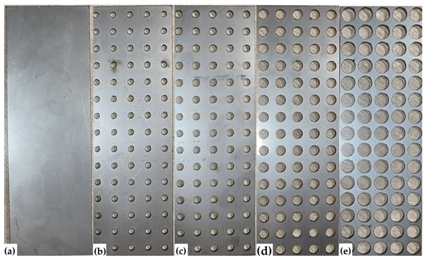
Figure 1.
Perforated stainless steel samples with a width of 150 mm, a length of 50 mm, and a thickness of 1 mm, prepared using the laser-cutting method. (a) Aperf = 0%; (b) Aperf = 7.07%; (c) Aperf = 12.56%; (d) Aperf = 23.75%; and (e) Aperf = 50.24%.
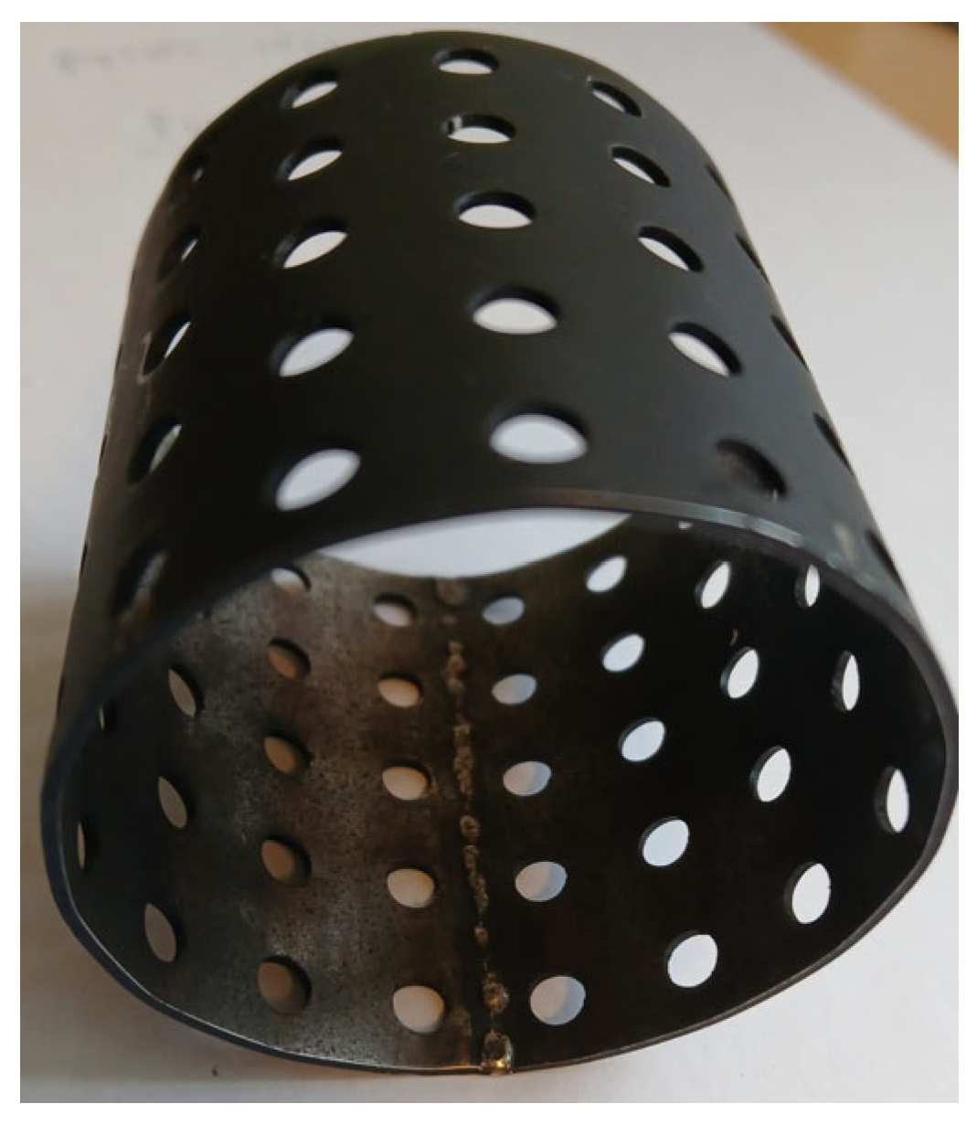
Figure 2.
Laser-welded perforated stainless-steel sample.
Figure 3.
Cylindrical specimens with a height of 50 mm, a thickness of 1 mm, and a diameter of 48 mm, produced by metal rolling and laser-welding methods. (a) Aperf = 0%; (b) Aperf = 7.07%; (c) Aperf = 12.56%; (d) Aperf = 23.75%; and (e) Aperf = 50.24%.
Figure 4.
Three-dimensional model of sample Nr. 5 and Nr. 3 obtained using 3D scanning.
Figure 5.
The “Polytec PSV 500 3D” setup is used for determining the frequency characteristics of the specimens. (a) Loudspeaker; (b) specimen; (c) controller; (d) distribution box; (e) PC; and (f) scanning head.
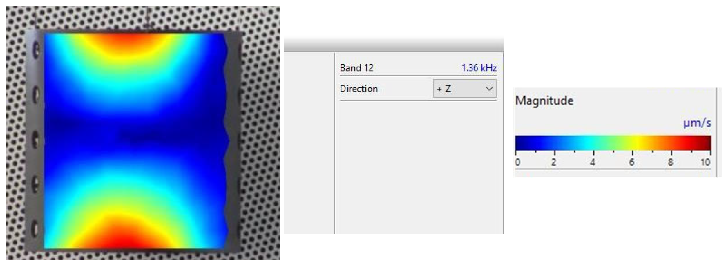
Figure 6.
An example of the obtained 4th resonance frequency and the corresponding mode shape for the studied specimen Nr. 3.
Figure 7.
Explanation of the experimental plan.
Figure 8.
Stabilization of resonance frequencies for the 1st studied sample.
Figure 9.
Dependence of the effective elastic modulus on the relative perforation area.
Figure 10.
Dependence of the effective shear modulus on the relative perforation area.
Table 1.
Perforation parameters for the stainless steel 304 plates.
| Sample Nr. | Perforation Diameter (mm) | Pitch Between Perforations (mm) | Relative Perforation Area (%) |
|---|
| 1. | - | - | - |
| 2. | 3 | 10 | 7.07 |
| 3. | 4 | 10 | 12.56 |
| 4. | 5.5 | 10 | 23.75 |
| 5. | 8 | 10 | 50.24 |
Table 2.
Physical, geometric, experimental, and calculated data of perforated stainless-steel 304 samples.
Sample
Nr. | Thickness
(m) | Length (m) | Width (m) | Mass
(kg) | Effective Specimen Density
(kg/m3) |
|---|
| 1. | 0.001 | 0.15 | 0.05 | 0.05711 | 7615 |
| 2. | 0.001 | 0.15 | 0.05 | 0.05311 | 7082 |
| 3. | 0.001 | 0.15 | 0.05 | 0.04973 | 6631 |
| 4. | 0.001 | 0.15 | 0.05 | 0.04299 | 5733 |
| 5. | 0.001 | 0.15 | 0.05 | 0.02713 | 3617 |
Table 3.
Finite element model convergence checks for the model of specimen Nr. 1.
| Resonance Frequency Number | Number of Finite Elements |
|---|
| 2 × 6 | 4 × 12 | 6 × 18 | 8 × 24 | 10 × 30 | 12 × 36 | 14 × 42 |
|---|
| Resonance Frequency Value, Hz |
|---|
| 1. | 1109 | 1090 | 1088 | 1088 | 1088 | 1088 | 1088 |
| 2. | 1113 | 1094 | 1092 | 1092 | 1091 | 1092 | 1092 |
| 3. | 1462 | 1447 | 1444 | 1443 | 1443 | 1443 | 1443 |
| 4. | 1469 | 1454 | 1451 | 1451 | 1450 | 1451 | 1451 |
| 5. | 3343 | 3100 | 3076 | 3072 | 3070 | 3071 | 3071 |
| 6. | 3421 | 3117 | 3095 | 3090 | 3088 | 3089 | 3088 |
| 7. | 3869 | 3662 | 3637 | 3633 | 3631 | 3632 | 3632 |
| 8. | 3969 | 3687 | 3664 | 3659 | 3657 | 3658 | 3657 |
| 9. | 7557 | 6057 | 5927 | 5900 | 5891 | 5889 | 5887 |
| 10. | 7917 | 6070 | 5932 | 5905 | 5897 | 5897 | 5894 |
| 11. | 8119 | 6708 | 6580 | 6554 | 6545 | 6543 | 6541 |
| 12. | 8521 | 6724 | 6588 | 6561 | 6552 | 6552 | 6550 |
| 13. | 13,883 | 10,143 | 9638 | 9538 | 9505 | 9496 | 9490 |
| 14. | 14,794 | 10,157 | 9661 | 9557 | 9524 | 9517 | 9509 |
| 15. | 17,322 | 10,826 | 10,327 | 10,228 | 10,196 | 10,186 | 10,181 |
Table 5.
Coefficients of the approximation function for specimen Nr. 1.
| Resonance Frequency Number | Number of Finite Elements |
|---|
| b0 | b1 | b2 | b11 | b12 | b22 | b0 |
|---|
| 1. | 290.92 | 5.38 × 10⁻⁹ | 5.59 | −8.51 × 10⁻²¹ | 1.77 × 10⁻⁹ | 3.93 | 290.92 |
| 2. | 383.38 | 7.89 × 10⁻⁹ | −1.80 | −1.11 × 10⁻²⁰ | −5.69 × 10⁻¹⁰ | −6.23 × 10⁻¹ | 383.38 |
| 3. | 385.33 | 7.93 × 10⁻⁹ | −1.82 | −1.12 × 10⁻²⁰ | −5.74 × 10⁻¹⁰ | −6.32 × 10⁻¹ | 385.33 |
| 4. | 818.22 | 1.51 × 10⁻⁸ | 15.57 | −2.39 × 10⁻²⁰ | 4.94 × 10⁻⁹ | 10.93 | 818.22 |
| 5. | 823.00 | 1.52 × 10⁻⁸ | 15.57 | −2.41 × 10⁻²⁰ | 4.94 × 10⁻⁹ | 10.93 | 823.00 |
| 6. | 965.63 | 1.92 × 10⁻⁸ | 3.34 | −2.81 × 10⁻²⁰ | 1.07 × 10⁻⁹ | 3.25 | 965.63 |
| 7. | 972.61 | 1.93 × 10⁻⁸ | 3.35 | −2.83 × 10⁻²⁰ | 1.07 × 10⁻⁹ | 3.24 | 972.61 |
| 8. | 1571.30 | 2.91 × 10⁻⁸ | 29.05 | −4.59 × 10⁻²⁰ | 9.21 × 10⁻⁹ | 20.32 | 1571.30 |
| 9. | 1572.60 | 2.92 × 10⁻⁸ | 29.04 | −4.60 × 10⁻²⁰ | 9.21 × 10⁻⁹ | 20.31 | 1572.60 |
| 10. | 1742.70 | 3.39 × 10⁻⁸ | 14.22 | −5.08 × 10⁻²⁰ | 4.51 × 10⁻⁹ | 10.77 | 1742.70 |
| 11. | 1744.40 | 3.39 × 10⁻⁸ | 14.23 | −5.08 × 10⁻²⁰ | 4.51 × 10⁻⁹ | 10.77 | 1744.40 |
| 12. | 2539.50 | 4.72 × 10⁻⁸ | 45.86 | −7.42 × 10⁻²⁰ | 1.45 × 10⁻⁸ | 31.92 | 2539.50 |
| 13. | 2544.60 | 4.73 × 10⁻⁸ | 45.63 | −7.44 × 10⁻²⁰ | 1.45 × 10⁻⁸ | 31.73 | 2544.60 |
| 14. | 2720.20 | 5.23 × 10⁻⁸ | 29.75 | −7.93 × 10⁻²⁰ | 9.44 × 10⁻⁹ | 21.33 | 2720.20 |
| 15. | 2726.00 | 5.24 × 10⁻⁸ | 29.78 | −7.95 × 10⁻²⁰ | 9.44 × 10⁻⁹ | 21.28 | 2726.00 |
Table 6.
Verification of approximation quality for each resonance frequency series of sample Nr. 1.
| | Resonance Frequency Order Number |
|---|
| 1 | 2 | 3 | 4 | 5 | 6 | 7 | 8 | 9 | 10 | 11 | 12 | 13 | 14 | 15 |
|---|
| Mean relative error, % | 0.59 | 0.47 | 0.47 | 0.58 | 0.58 | 0.47 | 0.47 | 0.57 | 0.57 | 0.48 | 0.48 | 0.57 | 0.56 | 0.5 | 0.5 |
| Maximum relative error, % | 1.82 | 1.21 | 1.21 | 1.81 | 1.8 | 1.19 | 1.19 | 1.77 | 1.77 | 1.35 | 1.35 | 1.74 | 1.74 | 1.44 | 1.44 |
| R2 value | 0.9993 | 0.9996 | 0.9996 | 0.9993 | 0.9993 | 0.9996 | 0.9996 | 0.9993 | 0.9994 | 0.9995 | 0.9995 | 0.9994 | 0.9994 | 0.9995 | 0.9995 |
Table 7.
The calculated results for the samples: effective elastic modulus and effective shear modulus.
| Sample Nr. | Effective Elastic Modulus (GPa) | Effective Shear Modulus (GPa) |
|---|
| 1. | 184.76 | 67.34 |
| 2. | 160.47 | 64.57 |
| 3. | 138.25 | 53.96 |
| 4. | 112.02 | 46.67 |
| 5. | 50.69 | 21.12 |
Table 8.
The calculated results of the specimens investigated are presented.
| Sample Nr. | Perforation Diameter (mm) | Relative Perforation Area (%) | Effective Elastic Modulus (GPa) | Effective Shear Modulus (GPa) |
|---|
| 1. | 0 | 0 | 184.76 | 67.34 |
| 2. | 3 | 7.07 | 160.47 | 64.57 |
| 3. | 4 | 12.56 | 138.25 | 53.96 |
| 4. | 5.5 | 23.75 | 112.02 | 46.67 |
| 5. | 8 | 50.24 | 50.69 | 21.12 |
| Disclaimer/Publisher’s Note: The statements, opinions and data contained in all publications are solely those of the individual author(s) and contributor(s) and not of MDPI and/or the editor(s). MDPI and/or the editor(s) disclaim responsibility for any injury to people or property resulting from any ideas, methods, instructions or products referred to in the content. |
© 2025 by the authors. Licensee MDPI, Basel, Switzerland. This article is an open access article distributed under the terms and conditions of the Creative Commons Attribution (CC BY) license (https://creativecommons.org/licenses/by/4.0/).
