The Time–Frequency Analysis and Prediction of Mold Level Fluctuations in the Continuous Casting Process

Abstract

Mold level fluctuation significantly affects the stability and quality of the slab during the continuous casting process. However, traditional mechanism models are insufficient for providing accurate time-series predictions under complex and multivariable operating conditions. Additionally, the dynamic interdependencies between process variables and transient abnormal fluctuation events have been largely overlooked in existing studies. To address these limitations, we propose an integrated time–frequency characterization and prediction framework that combines multi-domain feature extraction with a long-sequence Informer model. First, the preprocessing pipeline transforms heterogeneous sensor data into standardized time series through normalization and standardization, thereby establishing a robust foundation for subsequent feature extraction and predictive modeling. Second, the time–domain and frequency–domain feature extraction methods are integrated to capture essential patterns in casting signals with improved resolution and interpretability. Third, the fusion features are embedded into a time-series prediction model, which performs robust forecasting of mold level behavior and enhances the identification of root causes behind fluctuation anomalies. Compared with conventional LSTM and Transformer models, the proposed framework achieves over 90% reduction in prediction error and provides interpretable insights into the correlations between casting parameters and mold level variations. Finally, real industrial experimental results demonstrate the performance of the proposed framework in enhancing prediction reliability and providing insight into fluctuations with scalable implementation.

1. Introduction

Continuous casting technology has attracted increasing attention in modern steel manufacturing, which significantly influences both product quality and production efficiency [1,2]. The mold serves as a critical component of the continuous casting process by initiating the solidification of molten steel to directly affect the dimensional accuracy and internal integrity of the final product [3]. As illustrated in Figure 1, the structure of continuous casting structure and continuous casting mold, the design of the configuration and the mold structure is closely associated with the thermal and flow conditions within the casting zone. Among the various factors influencing casting stability, abnormal fluctuations in the molten steel level within the mold would cause surface defects and internal cracks during the solidification process [4]. Mold level fluctuation refers to the time–varying variation of the molten steel surface height within the mold during the continuous casting process. Stable control of the mold level is therefore essential for preventing defects and maintaining continuous and uniform solidification quality. There are three primary research subdirections for the real-time prediction of mold level fluctuations, including signal processing methods, traditional modeling techniques, and AI-based approaches.

Mold level stability impacted by a range of factors across the entire production chain is critical to both product quality and casting efficiency in continuous casting [5]. Signal processing is the primary technique task for real-time prediction of mold level fluctuations, the methods of which provide the practical foundation for subsequent modeling and intelligent analysis in industrial operations [6]. In the dynamic monitoring of mold level fluctuations during continuous casting, the main challenges involve extracting meaningful features and identifying fluctuation patterns from nonstationary and noise-corrupted signals. Current research predominantly employs the wavelet transform techniques and their variants, time–frequency joint analysis methods, and higher-order statistical computations for signal processing and analysis [7,8]. The wavelet transform is widely applied to the detection of transient disturbances and the suppression of nonlinear noise, due to its inherent capability for multiscale decomposition and localized signal analysis. The existing analytical framework can be broadly categorized into two methodological categories according to their processing principles: frequency–domain feature extraction based on discrete and continuous wavelet decomposition [9,10], and adaptive time–frequency analysis approaches such as empirical mode decomposition [11]. Wavelet-based methods demonstrate superior performance over traditional approaches in capturing complex and multimodal signals. However, inconsistencies in feature extraction processes and the absence of standardized multimodal integration frameworks impede effective quantitative analysis and precise system control. Therefore, transitioning toward dynamic time-series modeling is crucial to address these challenges.

Traditional modeling techniques demonstrate significant limitations in the control of the continuous casting process. Mechanism-based models frequently lack the adaptability required to accommodate complex and dynamic operating conditions, especially in situations involving multiple steel grades [12] and variable casting speeds [13,14]. Similarly, traditional linear time-series analysis methods exhibit limited responsiveness to nonlinear and transient disturbances in mold level fluctuations. The commonly employed PID control strategies in the secondary cooling zone [15] prove to be insufficient for addressing the unsteady-state heat transfer effects. These deficiencies fundamentally stem from the limited capacity of traditional models to capture the high-dimensional, nonlinear, and time-dependent relationships inherent in the casting process. However, traditional approaches often cannot adapt to the complex and transient operational conditions, thus limiting their practical effectiveness in real-world industrial applications.

Recent advancements in artificial intelligence, particularly in the domain of time-series forecasting, significantly reshape this landscape. Transformer architectures [16,17,18] that incorporate self-attention mechanisms have substantially enhanced the long-range prediction accuracy of critical process parameters. Spatiotemporal neural networks have facilitated the integrated modeling of multi-dimensional casting variables by effectively capturing both spatial topology and temporal evolution patterns, such as ConvLSTM [19,20]. Meanwhile, interpretable frameworks such as N-BEATS [21,22] facilitate transparent decision-making by leveraging trend and seasonal decomposition. In practical applications, hybrid deep learning models [23,24] have exhibited significant enhancements in predicting strand surface temperature distributions, thereby enabling more accurate thermal management [25]. Spatiotemporal graph attention networks further facilitate real-time monitoring and early warning of mold level fluctuations by dynamically correlating process parameters throughout the casting stages. Physics-informed neural networks, which incorporate fundamental heat transfer principles into data-driven architectures, provide advanced and optimized control strategies for secondary cooling water distribution, as validated by quantifiable improvements in strand surface quality. Collectively, these advancements suggest that AI-driven time-series modeling is successfully addressing the limitations of linearity and rigidity inherent in traditional control methodologies [17,26]. By combining advanced deep spatiotemporal feature extraction techniques with domain-specific physical knowledge, these models provide enhanced predictive capabilities and achieve superior control accuracy for continuous casting processes.

In addition to predictive modeling, recent optimization-oriented studies in metals have demonstrated complementary strategies for improving casting performance. For example, Brezina et al. compared meta-heuristic optimization algorithms for secondary cooling in continuous steel casting [27]. Brezocnik and Župerl optimized the continuous casting process of hypoeutectoid steel grades using multiple linear regression and genetic programming [28]. Yang et al. developed a digital-twin-based coordinated optimal control framework that integrates metaheuristic optimization and real-time feedback for continuous casting [29]. To extend the applicability of metaheuristic techniques, Rao and Davim (2025) investigated the optimization of different metal casting processes using three advanced algorithms, demonstrating their effectiveness across various casting environments [30]. In addition, Kovačič et al. applied genetic programming for billet-cooling optimization after continuous casting and verified the industrial scalability of the method [31]. These optimization approaches can be effectively combined with data-driven predictive frameworks, where predicted mold-level trends and cross-variable correlations serve as inputs or constraints for multi-objective control of casting speed, secondary-cooling intensity, and argon-flow regulation.

However, current methodologies lack comprehensive multi-factor fusion analysis of continuous casting data, which hinders their capacity to precisely capture and quantify multi-scale fluctuations of the mold level. Moreover, most existing data-driven approaches rely on single-domain features or shallow models, limiting their ability to describe nonlinear correlations and long-term dependencies under complex operating conditions. To overcome these limitations, this study proposes a unified time–frequency characterization and Informer-based prediction framework that bridges multi-domain feature analysis and intelligent forecasting for enhanced interpretability and industrial applicability.

In this article, the primary contributions can be succinctly summarized as follows:

• A novel time–frequency analysis and prediction framework is developed for mold level fluctuations in continuous casting, which can visualize and quantify dynamic correlations between fluctuation patterns and key process variables with improved interpretability.
• An integrated feature extraction strategy combining time–domain and frequency–domain analyses is utilized to identify the potential factors influencing mold level behavior and to reveal the coupling mechanisms between casting signals and liquid level responses.
• An Informer-based long-sequence prediction model is established to achieve accurate forecasting of mold level trends and to effectively suppress abnormal fluctuation events under multivariable casting conditions.
• Comprehensive validation using real industrial production data demonstrates that the proposed system achieves substantial improvement in prediction accuracy (over 90% reduction in MAE compared with baseline models) and provides a scalable solution for adaptive optimization of the continuous casting process.

The remainder of this paper is organized as follows. Section 2 provides an overview of the related work. In Section 3, we present the framework of the time–frequency analysis and predictions of mold level fluctuations in continuous casting processes. Section 4 delves into the details of the time series forecasting model. Section 5 concludes with future directions.

2. Related Work

Recently, a diverse range of signal processing and modeling techniques has been extensively utilized in the investigation of mold level control within continuous casting processes. A multiphase transient model for thin slab continuous casting molds has been developed to precisely simulate the asymmetric flow behavior of molten steel under various operating conditions. This model elucidates the influence of heat transfer and solidification processes on steel flow by comparing the flow field characteristics between three-dimensional (3D) and two-dimensional (2D) simulations.

To systematically analyze the wave characteristics and fluctuation frequencies in mold water models, the effective wave height combined with Fast Fourier Transform (FFT) analysis is utilized. Furthermore, Particle Image Velocimetry (PIV) measurements have been employed to investigate the coupling mechanism between flow field distributions and mold level fluctuations as reported in Reference [32]. The Continuous Wavelet Transform (CWT) has been demonstrated to be an effective tool for analyzing the time–frequency characteristics of instantaneous abnormal fluctuations in mold level and stopper rod displacements [33]. Additionally, the Discrete Wavelet Transform (DWT) algorithm has been utilized for the purpose of feature extraction and frequency classification in analyzing mold level fluctuations [34,35]. Although these conventional methods have made significant contributions, they are frequently limited by specific plant conditions and exhibit insufficient general applicability, thereby restricting their broad implementation in industrial contexts.

Numerous advanced time series forecasting methods have been developed and widely applied across various domains. For example, a Temporal Recurrent Neural Network (TRNN) model was proposed to effectively process and compress trading volume data, thereby substantially improving computational efficiency while maintaining prediction accuracy [36]. The Graphformer model introduces a novel graph attention mechanism as an alternative to traditional self-attention, facilitating the automatic learning of implicit sparse graph structures directly from raw data. This approach not only enhances the model’s generalization capability for time series that lack explicit graph structures but also effectively identifies latent spatial dependencies among sequences [37]. Empirical studies have demonstrated that this method attains near-optimal zero-shot prediction performance across multiple public datasets, competing with the accuracy of dataset-specific supervised models [38]. In parallel, a comprehensive analysis of Long Short-Term Memory (LSTM) networks has been carried out by dissecting individual computational components to systematically assess their contributions to forecasting performance [39,40]. However, it is important to highlight that the majority of these methods have primarily been utilized in traditional fields, such as meteorology and finance. In contrast, their incorporation and validation within industrial contexts remain relatively under investigated.

The rapid advancement of artificial intelligence (AI) technologies has significantly accelerated the development of a broad spectrum of innovative applications across various industrial sectors. One notable advancement is the Intelligent Adaptive Mold Level Fluctuation (IAMLF) predictive control method, which dynamically adjusts the stopper rod position in response to real-time mold level predictions, thus enabling more accurate level regulation [41]. Additionally, a convolutional neural network (CNN) model optimized via a genetic algorithm has been successfully implemented to develop a real-time prediction system for mold level fluctuations in continuous casting processes [42]. This system integrates feature heatmap visualization and Shapley Additive Explanations (SHAP) for a comprehensive analysis of the impact of various production parameters on mold level stability [43], as well as for quantitatively evaluating each parameter’s contribution to the model’s predictive performance [44,45]. Moreover, advanced deep learning-based intelligent fault diagnosis systems have been developed for critical components in the continuous casting process, including submerged entry nozzles and casting rollers. Nevertheless, it is crucial to emphasize that the implementation of intelligent methodologies for mold level fluctuation prediction remains comparatively constrained. Substantial research gaps continue to exist in this domain, underscoring the necessity for additional investigation and advancement.

3. Proposed Framework

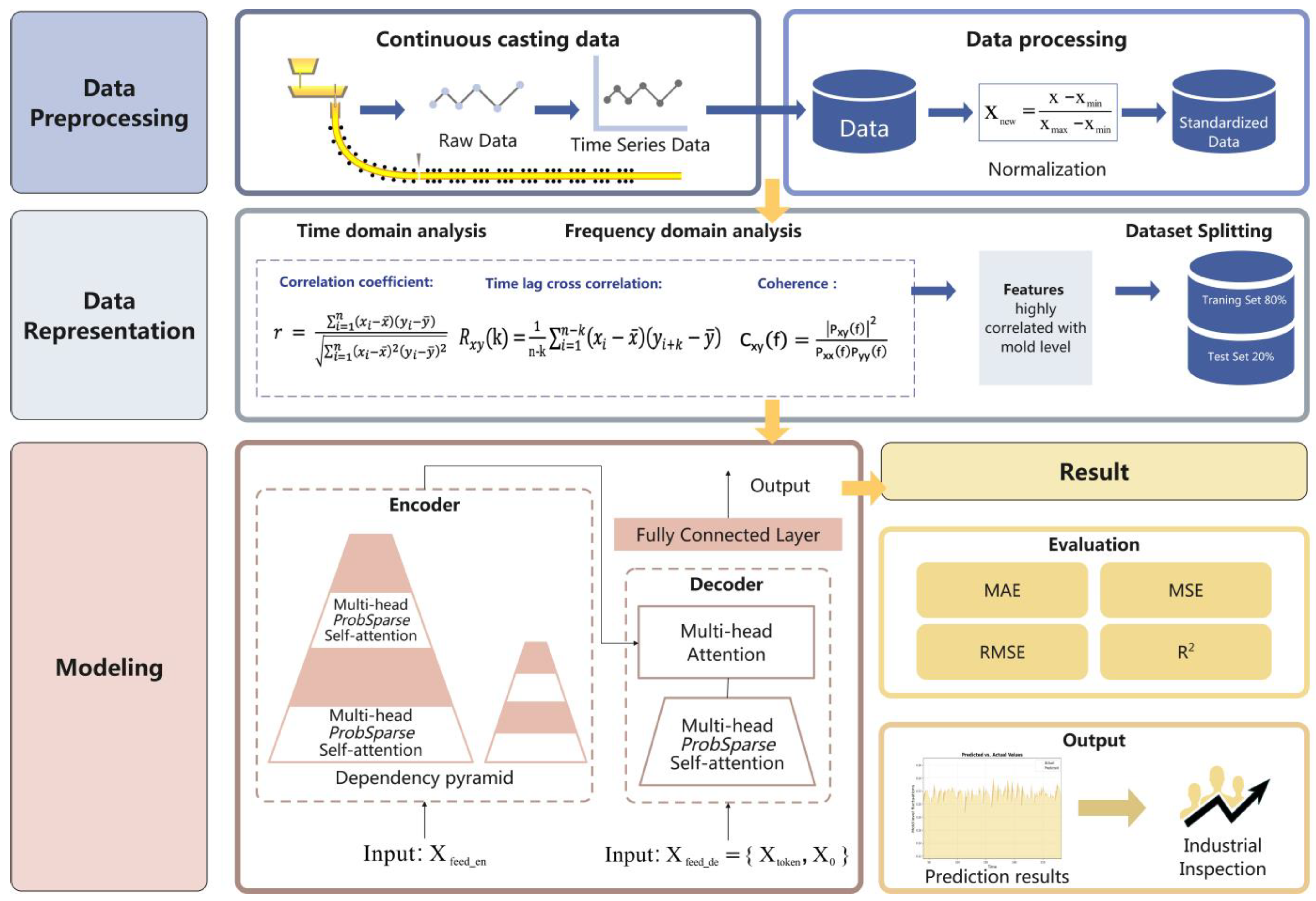
The predicting framework of mold level fluctuations in continuous casting processes is described in Figure 2. The framework of mold level fluctuation prediction system. which consists of four core modules, including continuous casting data preprocessing, data representation, mold level fluctuation time prediction, and predictive performance evaluation. Initially, the heterogeneous raw data acquired from various sensors within the facility are systematically arranged into time series according to the timestamps and heat numbers. These datasets are subsequently subjected to uniform normalization and standardization. Then, the preprocessed data are analyzed through multi-domain feature representation. This process identifies the most critical features correlated with mold level fluctuations, which are subsequently utilized as inputs for training the prediction model. For the prediction task, we employ the Informer model [46], which is a specialized architecture designed specifically for long-sequence time series forecasting. These core technologies are presented in the following subsections.

3.1. Data Preprocessing

In the data preprocessing stage, the heterogeneous raw signals collected from multiple sensors deployed within the continuous casting facility are first aggregated and systematically aligned according to their timestamps and heat numbers. This step ensures temporal coherence of the datasets and facilitates their transformation into structured time series representations suitable for subsequent analysis. To eliminate the influence of differing measurement scales and enhance comparability across variables, the aggregated data are subjected to normalization and standardization procedures.

Specifically, min–max normalization is employed to rescale each feature into a fixed interval, as defined by

$$x_{\mathrm{new}}={\displaystyle \frac{x-x_{min}}{x_{max}-x_{min}}}$$

(1)

where $x_{min}$ and $x_{max}$ denote the minimum and maximum values of the corresponding feature, respectively. In addition, Z-score standardization is adopted to transform features into a distribution with zero mean and unit variance, expressed as

$$x_{\mathrm{std}}={\displaystyle \frac{x-\mathsf{\mu }}{\mathsf{\sigma }}}$$

(2)

where $\mathsf{\mu }$ and $\mathsf{\sigma }$ represent the mean and standard deviation of the feature, respectively.

Through the preprocessing pipeline, the resulting standardized datasets exhibit consistent scales and statistical properties, thereby providing a robust and reliable foundation for subsequent feature extraction and predictive modeling.

Min–max normalization ensures numerical uniformity and accelerates convergence during model training, while Z-score standardization preserves inter-variable relationships by removing mean and variance bias. Their combined use provides balanced feature scaling across heterogeneous sensors.

The key continuous casting parameters used in this study are summarized in

Table 1. Definitions of key continuous casting parameters used in this study.

Parameter	Definition
Net weight	The net weight of molten steel in the tundish that is fed into the mold during the casting process. It represents the amount of steel available for casting. The identification number of the tundish car, which transports the tundish (the vessel holding molten steel) to the caster for continuous casting.
TC No (Tundish Car Number)
Pour length	The length of the casting, representing the portion of steel being continuously poured into the mold. It is critical for determining the quality of the steel slab or billet.
Argon pressure of Car 3	The argon gas pressure applied to Tundish Car 3. Argon is used to reduce gas bubble formation and control molten steel flow for smooth casting.
Argon pressure of Car 4	The argon gas pressure applied to Tundish Car 4, used similarly to regulate flow and prevent casting defects.
Argon flow rate of Car 3	The flow rate of argon gas in Tundish Car 3, which plays a similar role in controlling steel flow.
Argon flow rate of Car 4	The flow rate of argon gas in Tundish Car 4. Proper control of this flow rate helps stabilize the mold and improve casting uniformity.
Stopper gap	The opening of the stopper rod that controls molten steel flow from the tundish into the mold. This gap is critical for maintaining stable mold levels.
Width	The adjustable width of the cast product (slab or billet), influencing the overall geometry and surface quality.
Speed (Casting speed)	The linear withdrawal speed of the mold from the continuous casting machine, which directly affects solidification rate and product quality.
Mold level fluctuation	Mold level fluctuation refers to the time-varying oscillation of the molten steel surface height within the mold during the continuous casting process.

. These variables were continuously monitored during the casting process and serve as the input features for subsequent time–frequency analysis and prediction modeling.

3.2. Time Domain Analysis

The Pearson correlation coefficient, commonly denoted as $r$, is a statistical measure that quantifies the strength and direction of the linear relationship between the relative movements of two variables. The formula for calculating the Pearson correlation coefficient is presented by

$$r = {\displaystyle \frac{{\sum }_{i=1}^n\left(x_i-\overline{x}\right)\left(y_i-\overline{y}\right)}{\sqrt{{\sum }_{i=1}^n{\left(x_i-\overline{x}\right)}^2{\left(y_i-\overline{y}\right)}^2}}}$$

(3)

where $x_i$ and $y_i$ denote the individual sample points indexed with $i$, $\overline{x}$ and $\overline{y}$ represent the means of $x$ and $y,$ respectively, and $n$ is the total number of samples. The numerator denotes the covariance of $x$ and $y$, while the denominator corresponds to the product of the standard deviations of $x$ and $y$. The resulting coefficient is a value that ranges from $-1$ to $1$, inclusive. A value of $1$ indicates a perfect positive linear relationship, $-1$ indicates a perfect negative linear relationship, and $0$ indicates no linear relationship between the two variables.

The Pearson correlation coefficient is widely utilized in mathematics, statistics, and social sciences as a quantitative measure of the degree of linear dependence between two variables. All Pearson correlation coefficients are employed to quantify global synchronization, effectively condensing the relationship between two signals into a single value. However, continuous casting data may exhibit significant fluctuations during a casting stage, and a single value might not sufficiently capture the relationship between two variables. The Pearson coefficient provides a foundational calculation, which is complemented by other more precise methods to ensure a comprehensive analysis.

The time-lag cross-correlation method was employed to analyze the correlation between two time series. This approach allows for the quantification of the correlation between two signals and the determination of the delay in the effect of one signal on the other. The time-lag cross-correlation is computed as

$$R_{xy}\left(k\right)={\displaystyle \frac{1}{n-k}}{\displaystyle \sum _{i=1}^{n-k}}\left(x_i-\overline{x}\right)\left(y_{i+k}-\overline{y}\right)$$

(4)

where $k$ denotes the time-lag parameter, which represents the delay of $y$ relative to $x$ when computing the correlation between $x$ and $y$. $R_{xy}\left(k\right)$ represents the cross-correlation between $x$ and $y$ at a time lag of $k$, $n$ denotes the number of data points, $x_i$ and $y_i$ are the values of $x$ and $y$ at $i$-th time point, $\overline{x}$ and $\overline{y}$ represent the means of $x$ and $y$, respectively.

To enhance comprehension and provide a visual representation of the time-lag cross-correlation, a correlation plot can be constructed. The plot illustrates how the correlation between $x$ and $y$ varies under different time lags, thereby facilitating a deeper understanding of the dynamic relationship between two signals.

3.3. Frequency Domain Analysis

Specifically, coherence coefficients and time-lagged cross-correlation methods are employed in the time domain, whereas coherence analysis and continuous wavelet transform are utilized in the frequency domain.

Coherence is a metric that quantifies the linear relationship between two signals in the frequency domain, as it assesses the degree to which one signal can be predicted from another at various frequencies. The coherence function for two signals $x\left(t\right)$ and $y\left(t\right)$ is defined as follows:

$$C_{xy}\left(f\right)={\displaystyle \frac{{\left|P_{xy}\left(f\right)\right|}^2}{P_{xx}\left(f\right)P_{yy}\left(f\right)}}$$

(5)

where $P_{xy}\left(f\right)$ denotes the cross power spectral density of $x\left(t\right)$ and $y\left(t\right)$, while $P_{xx}\left(f\right)$ and $P_{yy}\left(f\right)$ represent the auto power spectral densities of $x\left(t\right)$ and $y\left(t\right)$, respectively. The coherence value varies within the range of $0$ to $1$, where a value of $1$ signifies a perfect linear relationship at a specific frequency, and a value of $0$ implies no relationship.

3.4. Informer

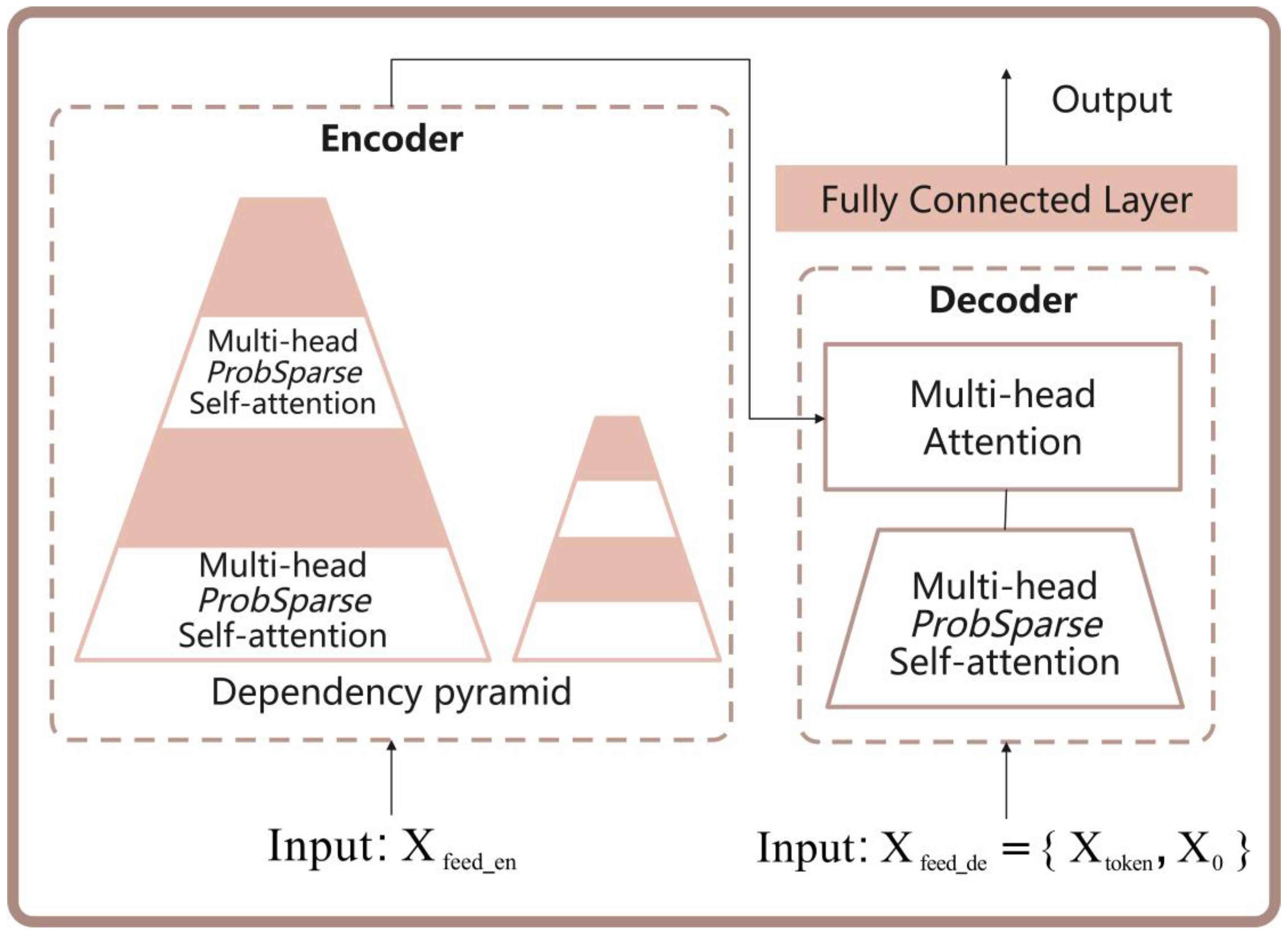
The Informer model embodies a pioneering deep learning architecture explicitly tailored for Long Sequence Time-Series Forecasting (LSTF). Through innovative modifications to the core components of the traditional Transformer framework, it achieves substantial reductions in computational complexity and memory usage while concurrently improving prediction accuracy and efficiency for long-term temporal dependencies. As depicted in Figure 3, the framework of the Informer-based mold level fluctuation prediction system, the architectural design of Informer centers on three key innovations: the Probabilistic Sparse Self-Attention Mechanism, the Self-Attention Distillation, and the Generative Decoder.

ProbSparse self-attention minimizes computational overhead by sparsifying attention operations. Self-attention distilling eliminates parameter redundancy through hierarchical feature compression. Layer stacking enhances robustness via progressive temporal pattern refinement. The system incorporates two key technologies: multi-domain data representation methods that extract discriminative features via hybrid time–frequency analysis, and an optimized Informer architecture that enables precise long-term fluctuation prediction. These two core technologies—multi-domain feature representation and the optimized Informer architecture—are elaborated in detail in the following subsections.

3.4.1. Probabilistic Sparse Self-Attention Mechanism

The probabilistic sparse self-attention mechanism constitutes a pivotal advancement in mitigating the computational inefficiency inherent in traditional Transformer architectures for long sequence modeling. Conventional self-attention mechanisms compute pairwise interactions between all queries $Q\in R^{L_Q\times d}$ and keys $K\in R^{L_K\times d}$, resulting in quadratic complexity $O\left(L_Q{L}_K\right)$. This renders such mechanisms prohibitively costly for sequences exceeding $L > 1000$ steps, thereby constraining their practicality in real-time industrial applications, including energy load forecasting and high-frequency financial prediction.

The fundamental innovation of this mechanism resides in its utilization of the long-tail distribution inherent in attention matrices. Empirical analyses demonstrate that, in most practical scenarios, only a limited subset of queries $q_i$ significantly contributes to the attention output, whereas the majority exert minimal influence. To formalize this insight, the sparse importance score $M\left(q_i,K\right)$ is introduced to quantify the deviation of each query’s attention distribution from uniformity as follows:

$$M\left(q_i,K\right)=\ln {\displaystyle \sum _{j=1}^{L_K}}{e}^{{\displaystyle \frac{q_i{k}_j^{\mathrm{\top }}}{\sqrt{d}}}}-{\displaystyle \frac{1}{L_K}}{\displaystyle \sum _{j=1}^{L_K}}{\displaystyle \frac{q_i{k}_j^{\mathrm{\top }}}{\sqrt{d}}}$$

(6)

where $q_i\in R^d$ is the $i$-th query vector and $k_j\in R^d$ is the $j$-th key vector. The first term captures the log-sum-exp of query-key interactions, reflecting the sparsity of dominant attention weights, while the second term computes their arithmetic mean to measure baseline uniformity. Queries with higher $M\left(q_i,K\right)$ values indicate stronger non-uniform attention patterns, signifying their critical role in temporal dependency modeling.

By selecting the top-$u$ queries $u=c\cdot \ln L_Q$, where $c$ is a hyperparameter controlling sparsity intensity, the mechanism constructs a sparse query matrix $\overline{Q}\in R^{u\times d}$. This enables the following sparsity-aware attention computation:

$$ProbSparseAttention\left(Q,K,V\right)=\mathrm{Softmax}\left({\displaystyle \frac{\overline{Q}{K}^{\mathrm{\top }}}{\sqrt{d}}}\right)V$$

(7)

where $V\in R^{L_V\times d}$ is the value matrix.

3.4.2. Self-Attention Distillation

To further address memory bottlenecks in multi-layer encoder architectures, the self-attention distillation technique hierarchically compresses intermediate feature representations through a pyramid-like structure. As encoder depth increases, this operation progressively eliminates redundant spatial- temporal features while preserving essential patterns critical for long-term forecasting.

3.4.3. Generative Decoder

The generative decoder adopts a parallel sequence generation paradigm to replace the traditional autoregressive decoding, effectively addressing the issues of error accumulation and inference latency. The system is built upon three principal components. First, the decoder input is constructed by hybridizing a segment of historical observations with future placeholders. Specifically, the most recent $L_x$ time steps of historical data $X_{t_c-L_x+1:t_c}\in R^{L_x\times d}$ are concatenated with zero-initialized future placeholders $0_{1:T}\in R^{T\times d}$ to form a composite matrix $X_{t_c-L_x+1:t_c}\in R^{L_x\times d}$, which serves as a structured input for parallel prediction. Second, a lower-triangular masking mechanism is introduced to constrain the attention scope, ensuring that each decoding step only attends to historical and current positions, thereby preventing information leakage from the future.

Finally, the decoder hidden states $H_{\mathrm{decoder}}\in R^{\left(L_x+T\right)\times d}$, produced by the masked ProbSparse self-attention mechanism, are directly projected into predicted future values through the following linear projection layer:

$$\widehat{Y_{1:T}}=W\cdot H_{\mathrm{decoder}}+b$$

(8)

where $W\in R^{d\times 1}$ and $b\in R$ are learnable parameters.

The proposed architecture reduces inference complexity to $O\left(1\right)$, fully decoupling prediction latency from the prediction horizon $T$. Moreover, the approach mitigates error accumulation typically observed in autoregressive models through a single end-to-end forward pass. Experimental results demonstrate that the generative decoder not only significantly improves inference efficiency but also effectively reduces cumulative error in long-term forecasting, offering an innovative solution that balances speed and accuracy for real-time long-horizon time series prediction tasks.

3.5. Evaluation Methods

The present study employs Mean Absolute Error ($MAE$), Mean Squared Error ($MSE$), Root Mean Squared Error ($RMSE$), and Coefficient of Determination ($R^2$) as performance evaluation metrics for the model. An $MAE$ that measures the average magnitude of absolute errors between the predicted values $\widehat{y_i}$ and the actual values $y_i$ is recorded as

$$MAE={\displaystyle \frac{1}{n}}{\displaystyle \sum _{i=1}^n}\left|y_i-\widehat{y_i}\right|$$

(9)

where $y_i$ represents the actual value of the $i$-th sample, and $\widehat{y_i}$ denotes the corresponding predicted value.

$MSE$ is a widely used metric in regression analysis to quantify the discrepancy between predicted and actual values. It calculates the average of the squared differences between predictions and true values, reflecting the magnitude of model errors. $MSE$ is recorded as

$$MSE={\displaystyle \frac{1}{n}}{\displaystyle \sum _{i=1}^n}{\left(y_i-\widehat{y_i}\right)}^2$$

(10)

An $RMSE$ that computes the square root of the mean squared error between predicted and actual values is given by

$$RMSE=\sqrt{{\displaystyle \frac{1}{n}}{\displaystyle \sum _{i=1}^n}{\left(y_i-\widehat{y_i}\right)}^2}$$

(11)

Compared with $MSE$, the $RMSE$ penalizes larger errors more severely due to the squaring operation.

The Mean Absolute Percentage Error (MAPE) measures the average relative error between the predicted values $\widehat{y_i}$ and the actual values $y_i$, expressed as a percentage. The MAPE provides an interpretable measure of prediction accuracy by quantifying the average deviation of predictions relative to actual values, making it particularly useful for comparing performance across datasets with different scales. The MAPE is given by

$$MAPE = {\displaystyle \frac{100\backslash \%}{n}}{\displaystyle \sum _{i=1}^n}\left|{\displaystyle \frac{y_i-\widehat{y_i}}{y_i}}\right|$$

(12)

where $y_i$ represents the actual value of the $i$-th sample, and $\widehat{y_i}$ denotes the corresponding predicted value.

4. Experiments and Results

4.1. Experimental Platform

In this study, a total of 210,000 data points are collected from a continuous twin-stream caster (China). The data is acquired at a sampling frequency of one data point per second. These data points are recorded using a set of sensors placed at various positions throughout the casting process, including sensors for monitoring casting speed, stopper control, and argon flow rate. All collected data are subject to preprocessing procedures to standardize the measurements. Specifically, min–max normalization is applied to rescale each feature to a fixed range between 0 and 1, and Z-score standardization is used to remove scale bias and maintain consistent distribution characteristics across the heterogeneous sensor data. During model training, the learning rate is set to 0.001, and the batch size is set to 32, which are commonly adopted configurations for time-series forecasting tasks to ensure stable convergence and efficient learning.

The dataset is then divided into two distinct sets, including training set to 80% of the data for training the model and testing set to 20% of the data for final evaluation to assess the model’s generalizability on unseen data. The input sequence length for the model is set to sixty time steps, with a label length of thirty and a prediction horizon of ten time steps. This configuration aims to balance model performance with prediction accuracy.

To evaluate the model’s stability and generalization capability, training is conducted over five iterations, and performance metrics are calculated after each iteration to track improvements. The training process also includes early stopping based on the validation set performance to avoid overfitting.

4.2. Results of Time Domain Analysis

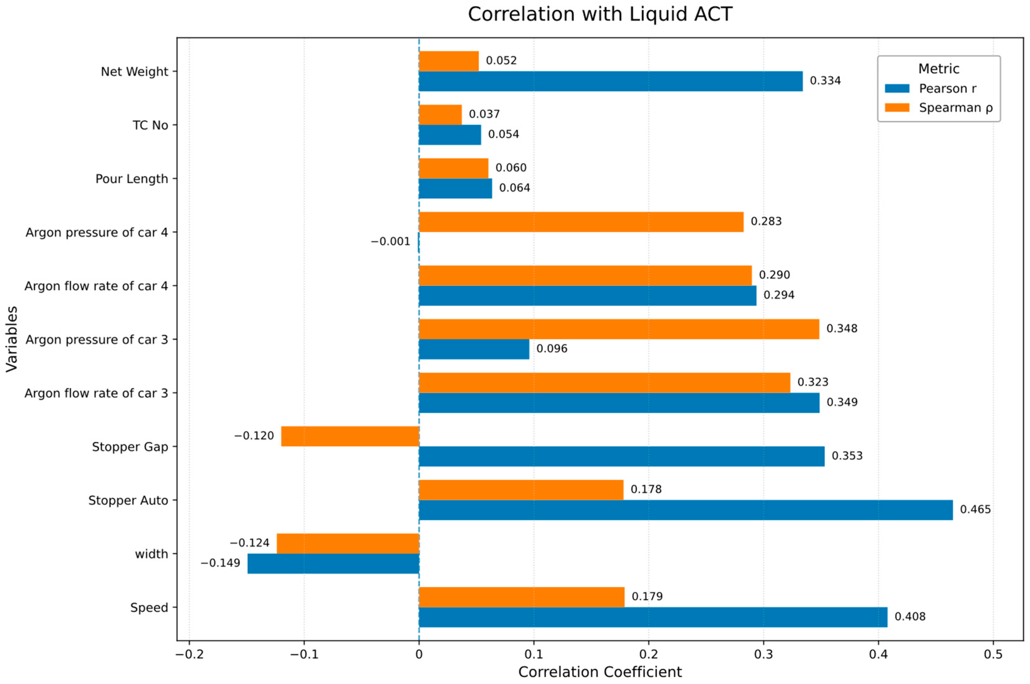
Figure 1 illustrates a comparative correlation analysis between mold level fluctuation values and multiple process parameters in continuous casting operations. Both Pearson and Spearman correlation coefficients are computed to quantify the type and intensity of these relationships.

As shown in Figure 4, the Pearson coefficient reflects the linear correlation strength, while the Spearman coefficient identifies monotonic but potentially nonlinear dependencies. The large discrepancies between them indicate nonlinear coupling effects among process parameters, particularly between argon flow rate and casting speed. This justifies the necessity of adopting a hybrid time–frequency analysis framework for comprehensive characterization.

Among the parameters evaluated, stopper auto exhibits the strongest linear correlation with mold level fluctuations (Pearson: 0.465). Similarly, casting speed demonstrates a strong positive correlation (Pearson: 0.408). Notably, the actual argon flow rate of three tapping rods and four tapping rods both show moderately strong correlations (Pearson: 0.349 and 0.294, respectively), reflecting the potential impact of argon flow regulation on mold level stability. These parameters may influence molten steel flow in the mold, which are recognized as primary causes of level fluctuations. In contrast, parameters such as width and stopper gap exhibit weak negative correlations (Pearson: −0.149; Spearman: −0.120). Collectively, stopper auto, casting speed, and argon flow rates demonstrate significant influences and should be prioritized for close monitoring or integration into predictive control models.

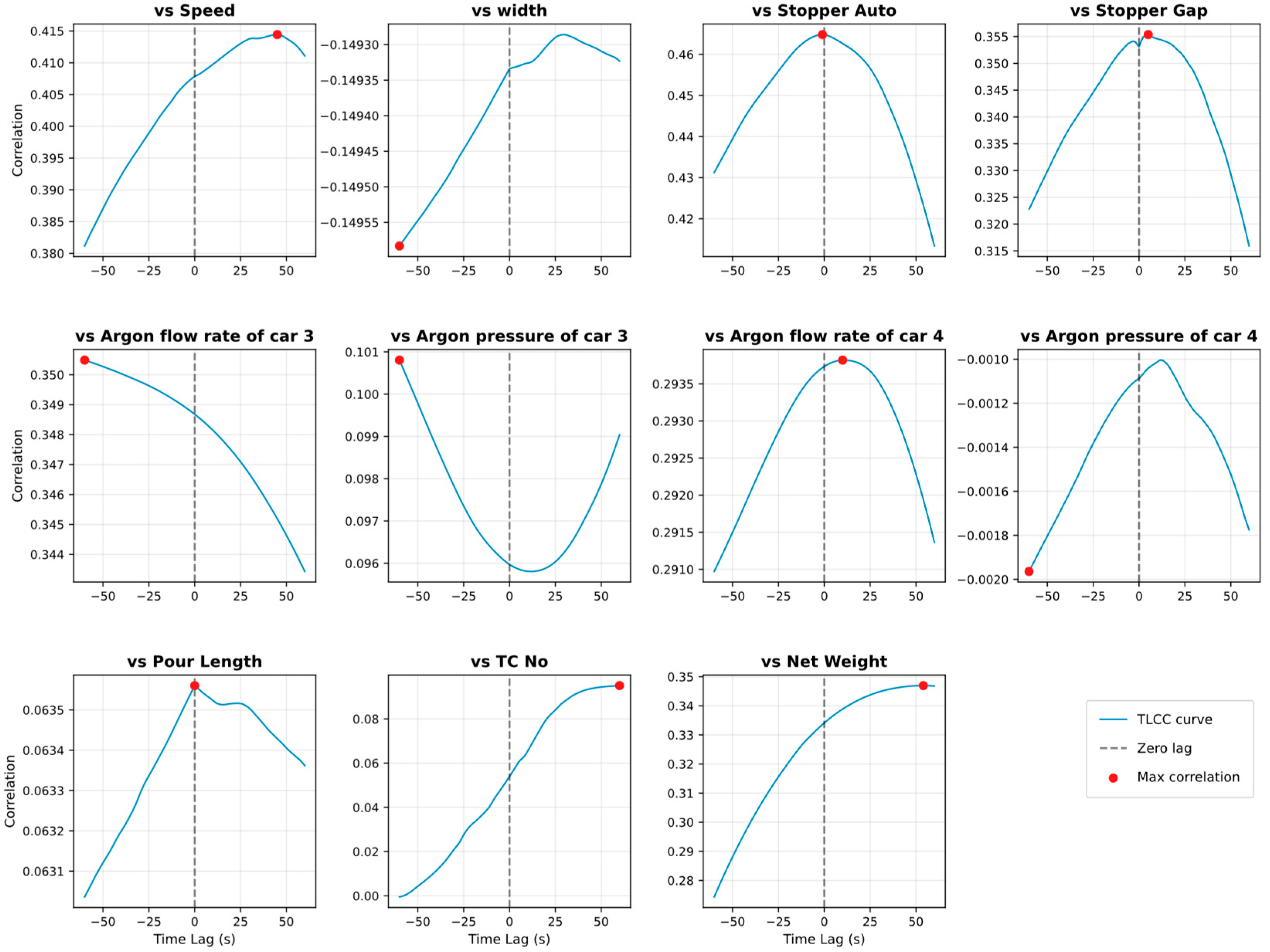
Figure 5 displays the time-lagged cross-correlation (TLCC) results between mold level fluctuations and key process parameters in continuous casting. Each subplot presents the correlation coefficient across different time lags (in seconds), where positive values indicate that the parameter precedes the fluctuation, while negative values suggest that it follows. Casting speed exhibits a peak correlation at approximately +50 s, indicating a delayed influence on mold level variations. The argon flow rate of car three shows a significant correlation at around −60 s, suggesting its potential as an early indicator of mold level instability. Notably, stopper auto demonstrates the highest correlation peak (~0.46), further supporting its critical role in mold level control. In contrast, certain parameters, such as the argon pressure of car four, exhibit minimal correlation, implying limited direct impact. Overall, the TLCC analysis identifies stopper auto, casting speed, and car three argon flow rate as the most significantly time-correlated parameters, offering valuable insights for prioritizing monitoring efforts and enhancing predictive control strategies.

Physically, the argon flow rate at car three interacts with the molten steel flow through a two-phase flow mechanism, where gas bubbles reduce the effective density of the steel jet, increasing the jet’s velocity and causing a pressure fluctuation at the mold meniscus. These pressure fluctuations are detected before visible changes occur in the mold level. According to momentum continuity and Bernoulli’s principle, the pressure variation $\Delta P$ caused by argon flow is given by the following equation:

$$\Delta P\approx \rho gh+{\displaystyle \frac{1}{2}}\rho v^2\left(1-{\alpha }_g\right)$$

(13)

where the terms are as defined previously. This pressure fluctuation is responsible for the early detection of instability, well before the mold level reaches a critical deviation.

4.3. Results of Frequency Domain Analysis

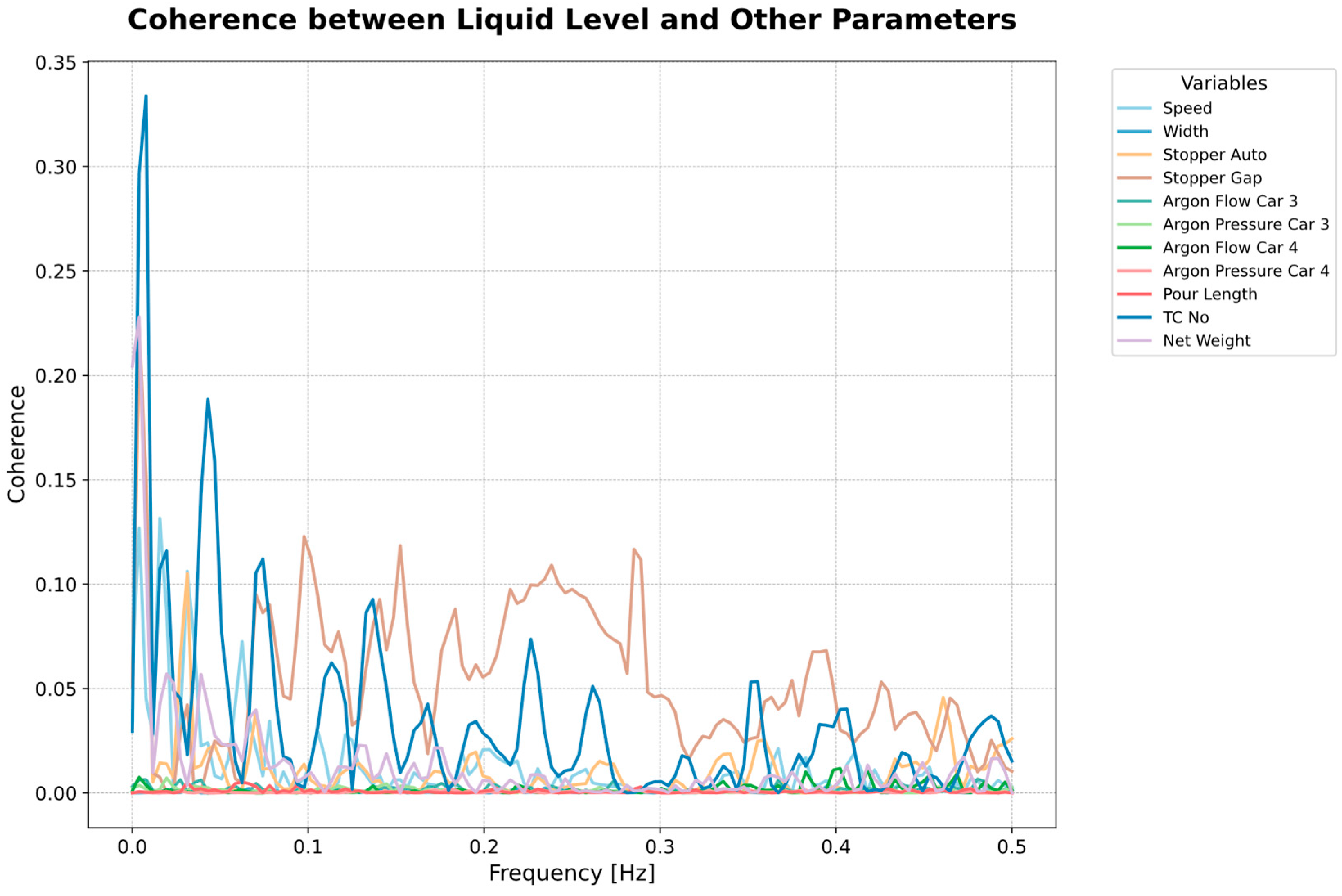
Figure 6 displays coherence spectra that illustrate the frequency–domain relationships between mold level fluctuations and various operational parameters during the continuous casting process. This coherence analysis reveals a strong linear relationship between mold liquid level fluctuations and the automatic stopper control system (Stopper Auto) within the critical 0.2–0.3 Hz frequency band (peak coherence ≈ 0.35), identifying it as the dominant influence on level stability. Casting speed shows a secondary, measurable relationship (peak coherence ≈ 0.25 at 0.2 Hz). All other parameters exhibit negligible coherence (<0.15) across the analyzed spectrum (0.1–0.5 Hz), indicating minimal linear correlation with level variations in this frequency range under the studied conditions. This highlights the primary importance of stopper control dynamics for level regulation.

In summary, the stopper auto setting, casting speed, and the actual argon flow rate of three tapping rod demonstrate significant correlations with mold level fluctuations in both the time and frequency domains. Identified factors serve as essential input variables within data-driven modeling frameworks, thereby facilitating more accurate prediction of mold level behavior during continuous casting processes.

4.4. Results of Three Deep Learning Models

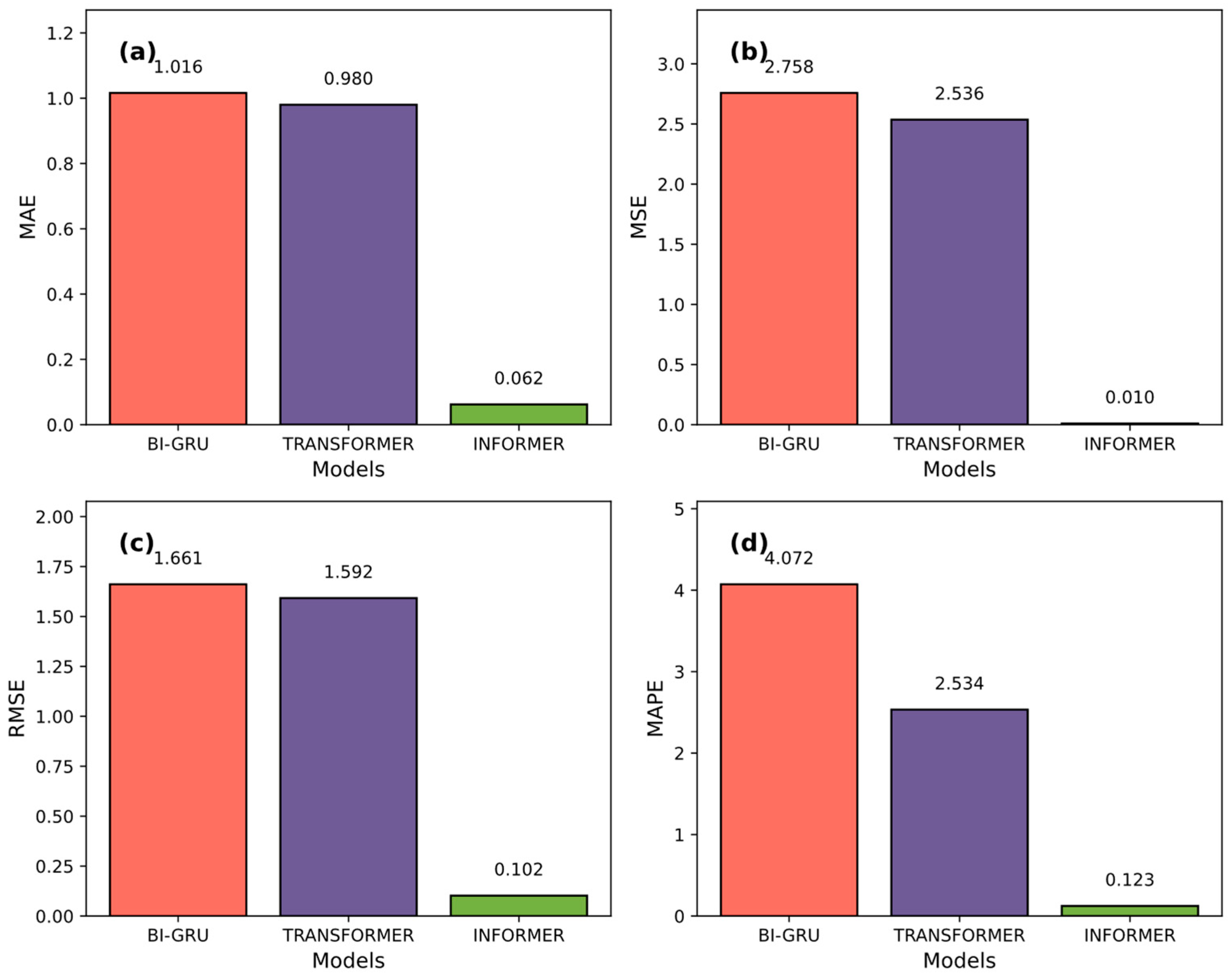
Figure 7 illustrates the prediction performance of three deep learning models evaluated by multiple metrics. As shown in Figure 7a, the Informer model exhibits a significantly lower Mean Absolute Error (MAE) than the other two models: Bi-GRU and Transformer achieve MAE values of 1.016 and 0.980, respectively, while the Informer achieves a notably lower MAE of 0.062, demonstrating a substantial improvement in prediction accuracy. Figure 7b shows a similar trend for Mean Squared Error (MSE): Bi-GRU and Transformer yield MSE values of 2.758 and 2.536, whereas Informer achieves an MSE of only 0.010, highlighting its superiority in minimizing prediction error variance. In Figure 7c, the Root Mean Squared Error (RMSE) results further confirm the Informer’s dominance, with RMSE values of 1.661 and 1.592 for Bi-GRU and Transformer, respectively, and where the Informer achieves a significantly lower RMSE of 0.102, indicating more stable predictions. Finally, Figure 7d displays the Mean Absolute Percentage Error (MAPE), where Informer achieves the lowest value of 0.123—substantially outperforming Transformer (2.534) and Bi-GRU (4.072). Collectively, the experimental findings demonstrate that the Informer model excels in both accuracy and robustness across all evaluation metrics.

It should be noted that the model’s predictive accuracy may decline when testing conditions differ substantially from the training domain, for example, under unseen casting speeds or steel grades. Such extrapolation introduces distributional shifts that increase prediction uncertainty. Future work will address this limitation by integrating domain adaptation and transfer learning strategies to enhance model generalization under varying operating conditions.

4.5. Results of Different Input Strategies Evaluated Using Multiple Metrics

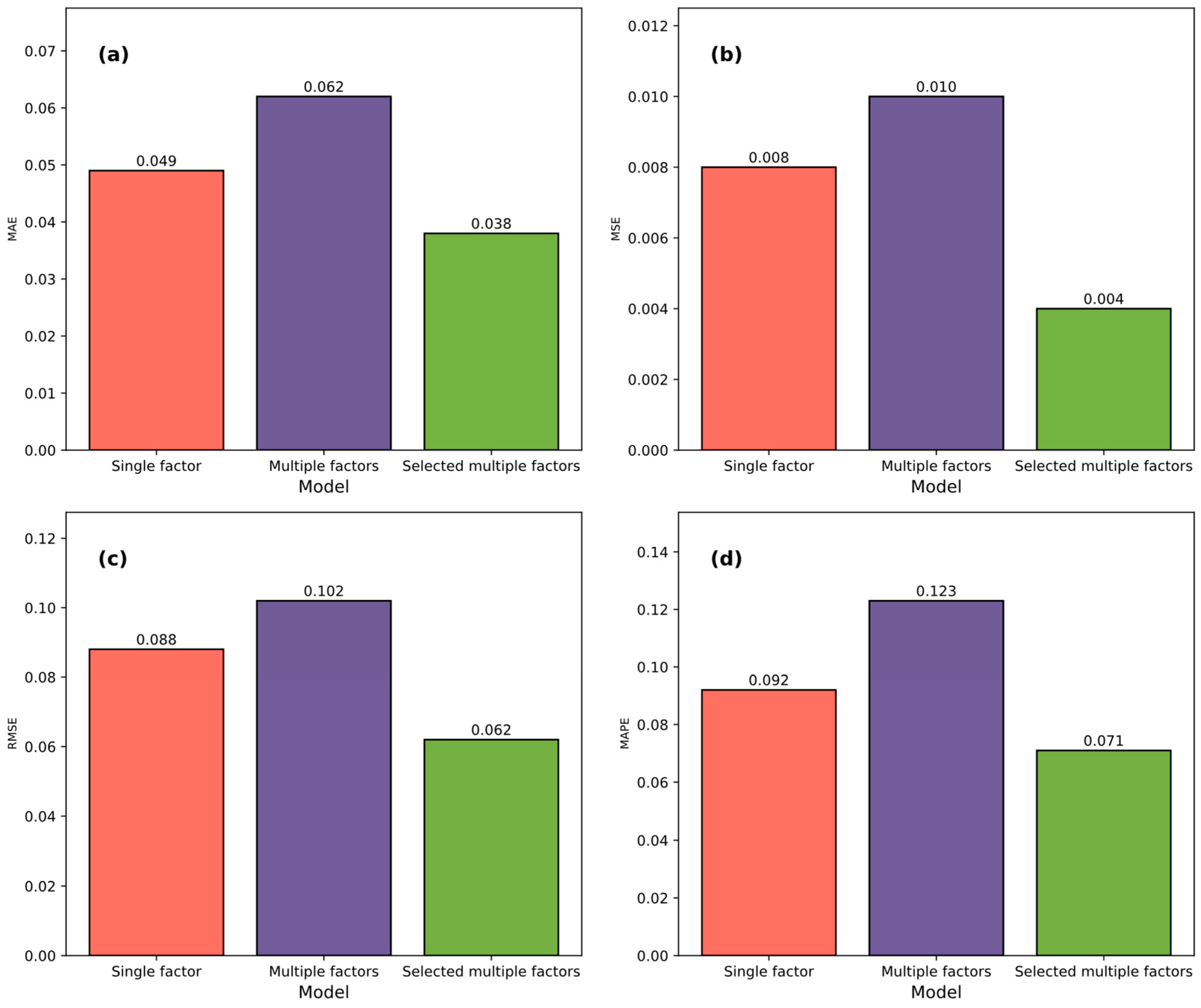
Figure 8 presents the prediction performance of different input strategies evaluated using multiple metrics. As shown in Figure 8a, the model incorporating selected multiple factors achieves the lowest MAE of 0.038, compared to 0.049 for the single-factor strategy and 0.062 for the unselected multi-factor strategy. This indicates that feature selection reduces absolute errors and enhances prediction accuracy. In Figure 8b, the selected multiple factors strategy yields the best MSE result (0.004), significantly lower than the single-factor (0.008) and unselected multi-factor (0.010) configurations, suggesting that refined input features mitigate prediction error variance. Figure 8c shows consistent trends in RMSE. The selected multiple factors strategy achieves an RMSE of 0.062, outperforming both the single-factor (0.088) and unselected multi-factor (0.102) approaches, which further validates improved prediction stability. Figure 8d displays MAPE values, where the selected multiple factors model records the lowest MAPE (0.071), while the unselected multi-factor model exhibits the highest (0.123), indicating that feature selection enhances robustness and reduces relative prediction errors. The consistent improvement across all metrics underscores the effectiveness of input factor selection in enhancing model generalization and predictive performance.

Figure 7 and Figure 8 collectively demonstrate that the Informer model outperforms Bi-GRU and Transformer across all evaluation metrics (MAE, MSE, RMSE, MAPE), with the lowest errors attributed to its efficiency in long-sequence time-series forecasting. Additionally, the input strategy incorporating selected multiple factors (e.g., stopper auto, casting speed, car three argon flow rate) consistently achieves superior prediction performance compared to single-factor or unselected multi-factor approaches, highlighting the critical role of feature selection in enhancing model accuracy and robustness.

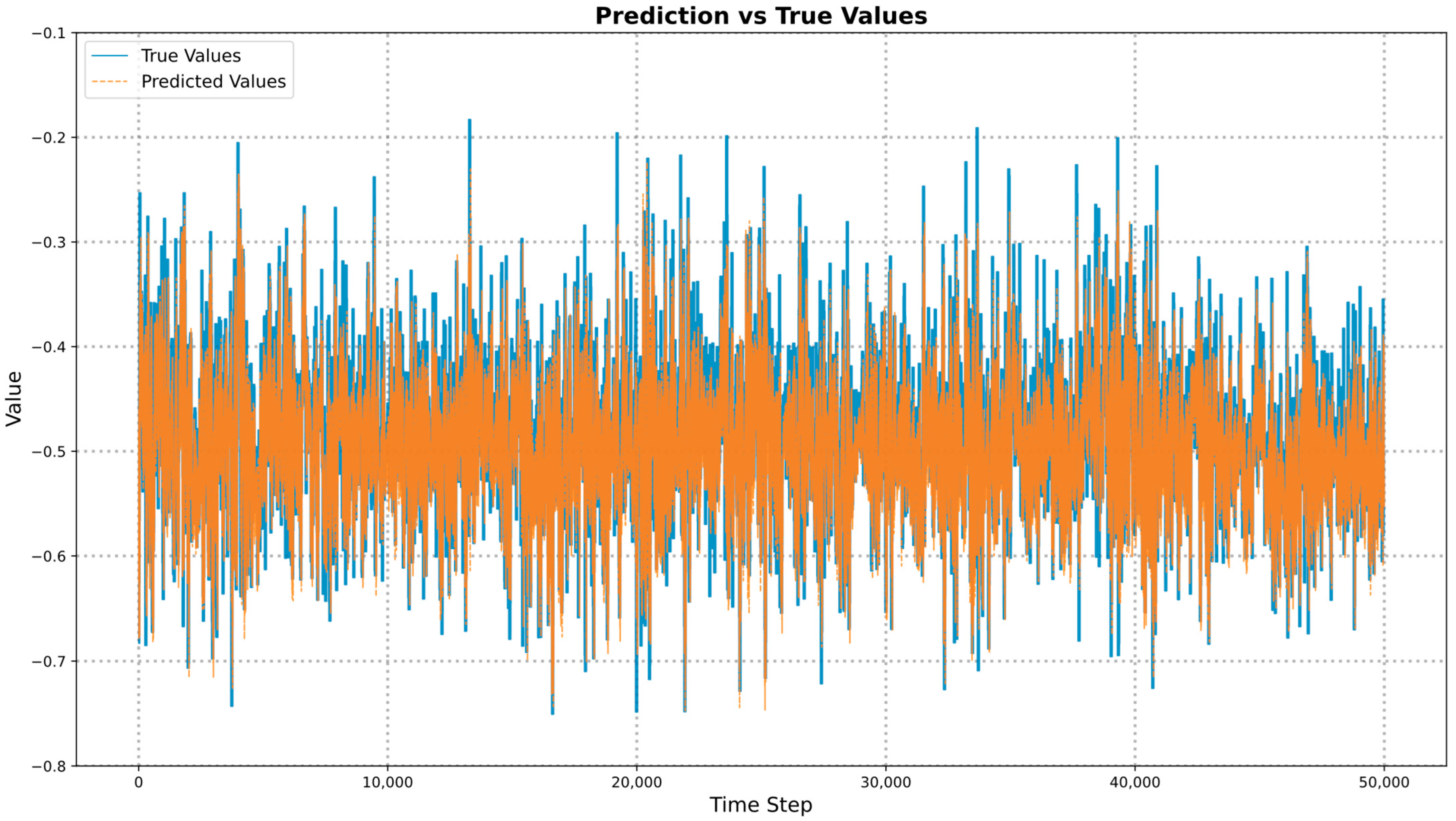
Notably, Figure 9 presents the time prediction results of the Informer model trained on the filtered features, showcasing the optimal performance among all tested configurations, which validates the effectiveness of integrating domain-informed feature selection with advanced deep learning architectures for mold level fluctuation forecasting in continuous casting.

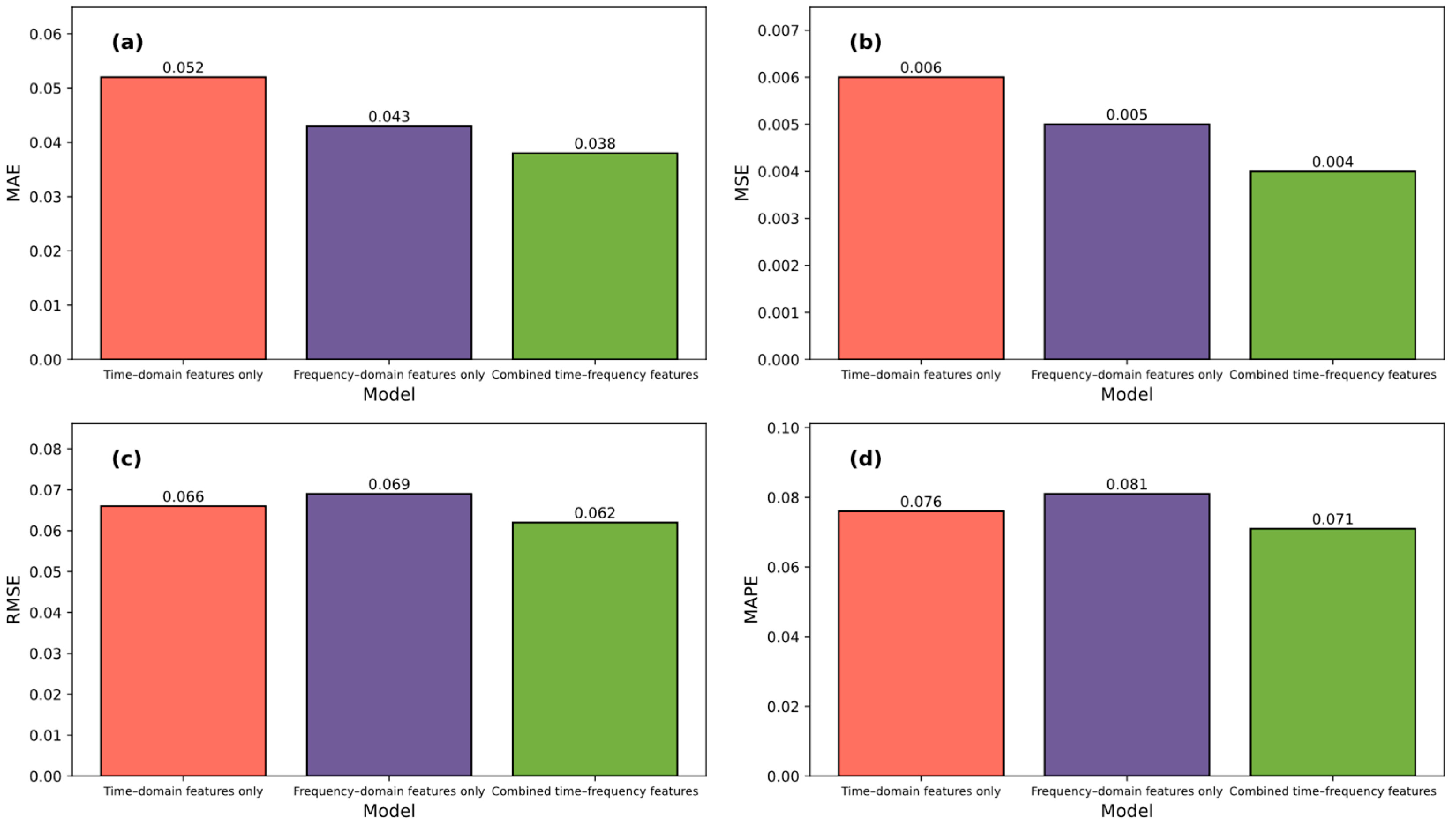
To assess the individual contributions of time–domain and frequency–domain features, we conducted an ablation analysis by training three models: one using time–domain features only, another using frequency–domain features only, and a final model using combined time–frequency features. Figure 10 presents the comparison of model performance across multiple evaluation metrics: MAE, MSE, RMSE, and MAPE.

As shown in Figure 10, the model incorporating combined time–frequency features consistently outperforms the models using time–domain features only or frequency–domain features only. Specifically, the model that uses time–domain features only shows higher error rates across all metrics, while the model using frequency–domain features only performs slightly better but still lags behind the model that uses combined time–frequency features. The combined features model achieves the lowest errors in all metrics, highlighting the complementary advantages of combining both time–domain and frequency–domain features for improved accuracy and robustness.

5. Conclusions

This paper presents an innovative system for analyzing and predicting mold level fluctuations through the integration of time–frequency analysis and machine learning methodologies. Unlike traditional single-domain or purely data-driven approaches, the proposed framework unifies multi-domain feature characterization and an Informer-based long-sequence forecasting model to achieve interpretable and high-precision prediction of mold level behavior. By extracting multiscale features and incorporating them into advanced deep learning models, the proposed method enhances both anomaly detection capabilities and predictive accuracy. Experimental comparisons indicate that the proposed framework achieves more than 90% reduction in mean absolute error (MAE) compared with conventional LSTM and Transformer models, validating its superior performance and robustness. The proposed framework has been rigorously validated using real-world production data, demonstrating its robust applicability in industrial settings and its potential for guiding adaptive process optimization in continuous casting operations.

In future activities, we will emphasize integrating a broader range of sensor data to improve system resilience under complex casting conditions, such as temperature fields and flow signals. The proposed predictive framework can also be integrated with recent optimization and control strategies reported in metals, including genetic programming-based cooling optimization, digital-twin-driven coordinated control, and reinforcement-learning-based casting regulation. Such integration will allow the predicted mold-level trends and correlation features to serve as inputs for adaptive optimization of secondary cooling and mold flow. Additionally, physics-informed modeling will be investigated to reinforce the synergy between empirical data and underlying physical processes. Furthermore, the deployment of the system for real-time monitoring and its integration with adaptive control logic will facilitate the development of autonomous, intelligent continuous casting systems.

References

1. Saini, D.K.; Jha, P.K. Fabrication of aluminum metal matrix composite through continuous casting route: A review and future directions. J. Manuf. Process. 2023, 96, 138–160. [Google Scholar] [CrossRef]
2. Li, C.; Zhang, T.; Liu, Y.; Liu, J. Effect of process parameters on surface quality and bonding quality of brass cladding copper stranded wire prepared by continuous pouring process for clad. J. Mater. Res. Technol. 2023, 26, 8025–8035. [Google Scholar] [CrossRef]
3. Li, Q.; Wen, G.; Chen, F.; Tang, P.; Hou, Z.; Mo, X. Irregular initial solidification by mold thermal monitoring in the continuous casting of steels: A review. Int. J. Miner. Metall. Mater. 2024, 31, 1003–1015. [Google Scholar] [CrossRef]
4. Zhao, P.; Li, Q.; Kuang, S.B.; Zou, Z. LBM-LES simulation of the transient asymmetric flow and free surface fluctuations under steady operating conditions of slab continuous casting process. Metall. Mater. Trans. B 2017, 48, 456–470. [Google Scholar] [CrossRef]
5. Zhang, Q. Numerical simulation of influence of casting speed variation on surface fluctuation of molten steel in mold. J. Iron Steel Res. Int. 2010, 17, 15–19. [Google Scholar] [CrossRef]
6. Lei, H.; Liu, J.; Tang, G.; Zhang, H.; Jiang, Z.; Lv, P. Deep insight into mold level fluctuation during casting different steel grades. JOM 2023, 75, 914–919. [Google Scholar] [CrossRef]
7. Ma, Y.; Fang, B.; Ding, Q.; Wang, F. Analysis of mold friction in a continuous casting using wavelet transform. Metall. Mater. Trans. B 2018, 49, 558–568. [Google Scholar] [CrossRef]
8. Yong, M.; Fangyin, W.; Cheng, P.; Wei, G.; Bohan, F. Analysis of Mold Friction in a Continuous Casting Using Wavelet Entropy. Metall. Mater. Trans. B 2016, 47, 1565–1572. [Google Scholar] [CrossRef]
9. Wei, Z.J.; Wang, T.; Feng, C.; Li, X.-Y.; Liu, Y.; Wang, X.-D.; Yao, M. Modeling and Simulation of Multi-phase and Multi-physical Fields for Slab Continuous Casting Mold Under Ruler Electromagnetic Braking. Metall. Mater. Trans. B 2024, 55, 2194–2208. [Google Scholar] [CrossRef]
10. Jin, Y.; Luo, S.; Meng, X.; Liu, Z.; Wang, C.; Wang, W.; Zhu, M. A Real-Time Prediction Method for Heat Flux in Continuous Casting Mold with Optical Fibers. Metall. Mater. Trans. B 2025, 56, 1865–1878. [Google Scholar] [CrossRef]
11. Xie, Z.; Yu, D.; Zhan, C.; Zhao, Q.; Wang, J.; Liu, J.; Liu, J. Ball screw fault diagnosis based on continuous wavelet transform and two-dimensional convolution neural network. Meas. Control 2023, 56, 518–528. [Google Scholar] [CrossRef]
12. Yang, W.; Zhang, L.; Ren, Y.; Chen, W.; Liu, F. Formation and prevention of nozzle clogging during the continuous casting of steels: A review. ISIJ Int. 2024, 64, 1–20. [Google Scholar] [CrossRef]
13. Dong, X.; Li, L.; Tang, Z.; Huang, L.; Liu, H.; Liao, D.; Yu, H. The Effect of Continuous Casting Cooling Process on the Surface Quality of Low-Nickel Austenitic Stainless Steel. Steel Res. Int. 2025, 2400957, 108–117. [Google Scholar] [CrossRef]
14. Guo, D.; Zeng, Z.; Peng, Z.; Guo, K.; Hou, Z. Effect of Casting Speed on CET Position Fluctuation Along the Casting Direction in Continuous Casting Billets. Metall. Mater. Trans. B 2023, 54, 450–464. [Google Scholar] [CrossRef]
15. Landauer, J.; Marko, L.; Kugi, A.; Steinboeck, A. Mathematical modeling and system analysis for preventing unsteady bulging in continuous slab casting machines. J. Process Control 2024, 139, 103232. [Google Scholar] [CrossRef]
16. Han, K.; Xiao, A.; Wu, E.; Guo, J.; Xu, C.; Wang, Y. Transformer in transformer. Adv. Neural Inf. Process. Syst. 2021, 34, 15908–15919. [Google Scholar]
17. Deng, Z.; Zhang, Y.; Zhang, L.; Cong, J. A Transformer and Random Forest Hybrid Model for the Prediction of Non-metallic Inclusions in Continuous Casting Slabs. Integr. Mater. Manuf. Innov. 2023, 12, 466–480. [Google Scholar] [CrossRef]
18. Fang, X.; Liu, C.; Yang, H.; Zheng, X.; Chen, X. Noise-Reduced Anomaly Attention Transformer for Intelligent Microscale Defects Detection in Metal Materials. IEEE Trans. Instrum. Meas. 2024, 73, 6505313. [Google Scholar] [CrossRef]
19. Zhang, C. Application of neural network in steelmaking and continuous casting: A review. Ironmak. Steelmak. 2024, 03019233241301144. [Google Scholar] [CrossRef]
20. Sun, F.; Jin, W. CAST: A convolutional attention spatiotemporal network for predictive learning. Appl. Intell. 2023, 53, 23553–23563. [Google Scholar] [CrossRef]
21. Yang, R.; Cao, L.; Li, J.; Yang, J. Variational Hierarchical N-BEATS Model for Long-term Time-series Forecasting. IEEE Trans. Neural Netw. Learn. Syst. 2025, 36, 19398–19410. [Google Scholar] [CrossRef]
22. Van Belle, J.; Crevits, R.; Caljon, D.; Verbeke, W. Probabilistic forecasting with modified N-BEATS networks. IEEE Trans. Neural Netw. Learn. Syst. 2024, 35, 18872–18885. [Google Scholar] [CrossRef]
23. Zhou, Y.; Xu, K.; He, F.; Zhang, Z. Application of time series data anomaly detection based on deep learning in continuous casting process. ISIJ Int. 2022, 62, 689–698. [Google Scholar] [CrossRef]
24. Yang, H.; Fang, Y.; Liu, L.; Ju, H.; Kang, K. Improved YOLOv5 based on feature fusion and attention mechanism and its application in continuous casting slab detection. IEEE Trans. Instrum. Meas. 2023, 72, 1–16. [Google Scholar] [CrossRef]
25. Wang, T.; Li, K.; Li, S.; Wang, L.; Yang, J.; Feng, L. Asymmetric flow behavior of molten steel in thin slab continuous casting mold. Metall. Mater. Trans. B 2023, 54, 3542–3553. [Google Scholar] [CrossRef]
26. Sun, Y.; Liu, Z.; Xiong, Y.; Yang, J.; Xu, G.; Li, B. A Novel Feedforward Neural Network Model for Predicting the Level Fluctuation in Continuous Casting Mold. Metall. Mater. Trans. B 2025, 56, 5009–5026. [Google Scholar] [CrossRef]
27. Brezina, M.; Mauder, T.; Klimes, L.; Stetina, J. Comparison of Optimization-Regulation Algorithms for Secondary Cooling in Continuous Steel Casting. Metals 2021, 11, 237. [Google Scholar] [CrossRef]
28. Brezocnik, M.; Župerl, U. Optimization of the Continuous Casting Process of Hypoeutectoid Steel Grades Using Multiple Linear Regression and Genetic Programming—An Industrial Study. Metals 2021, 11, 972. [Google Scholar] [CrossRef]
29. Yang, J.; Ji, Z.; Liu, W.; Xie, Z. Digital-Twin-Based Coordinated Optimal Control for Steel Continuous Casting Process. Metals 2023, 13, 816. [Google Scholar] [CrossRef]
30. Rao, R.V.; Davim, J.P. Optimization of Different Metal Casting Processes Using Three Simple and Efficient Advanced Algorithms. Metals 2025, 15, 1057. [Google Scholar] [CrossRef]
31. Kovačič, M.; Zupanc, A.; Vertnik, R.; Župerl, U. Optimization of Billet Cooling after Continuous Casting Using Genetic Programming—Industrial Study. Metals 2024, 14, 819. [Google Scholar] [CrossRef]
32. Wang, Z.; Shan, Q.; Gao, Y.; Pan, H.; Lu, B.; Wen, J.; Cui, H. Physical Simulation of Mold Level Fluctuation Characteristics. Metall. Mater. Trans. B 2023, 54, 2591–2604. [Google Scholar] [CrossRef]
33. Meng, X.; Luo, S.; Zhou, Y.; Wang, W.; Zhu, M. Time–Frequency Characteristics and Predictions of Instantaneous Abnormal Level Fluctuation in Slab Continuous Casting Mold. Metall. Mater. Trans. B 2023, 54, 2426–2438. [Google Scholar] [CrossRef]
34. Wang, Z.; Shan, Q.; Cui, H.; Pan, H.; Lu, B.; Shi, X.; Wen, J. Characteristic analysis of mold level fluctuation during continuous casting of Ti-bearing IF steel. J. Mater. Res. Technol. 2024, 31, 1367–1378. [Google Scholar] [CrossRef]
35. Wang, Z.; Wang, R.; Liu, J.; Yu, W.; Li, G.; Cui, H. Exploration of the causes of abnormal mold level fluctuation in thin slab continuous casting mold. J. Mater. Res. Technol. 2024, 33, 1460–1469. [Google Scholar] [CrossRef]
36. Lu, M.; Xu, X. TRNN: An efficient time-series recurrent neural network for stock price prediction. Inf. Sci. 2024, 657, 119951. [Google Scholar] [CrossRef]
37. Wang, Y.; Long, H.; Zheng, L.; Shang, J. Graphformer: Adaptive graph correlation transformer for multivariate long sequence time series forecasting. Knowl.-Based Syst. 2024, 285, 111321. [Google Scholar] [CrossRef]
38. Das, A.; Kong, W.; Sen, R.; Zhou, Y. A decoder-only foundation model for time-series forecasting. In Proceedings of the Forty-first International Conference on Machine Learning, Vienna, Austria, 21–27 July 2024. [Google Scholar]
39. Yadav, H.; Thakkar, A. NOA-LSTM: An efficient LSTM cell architecture for time series forecasting. Expert Syst. Appl. 2024, 238, 122333. [Google Scholar] [CrossRef]
40. Hochreiter, S.; Schmidhuber, J. Long short-term memory. Neural Comput. 1997, 9, 1735–1780. [Google Scholar] [CrossRef]
41. Meng, X.; Luo, S.; Zhou, Y.; Wang, W.; Zhu, M. Control of Instantaneous Abnormal Mold Level Fluctuation in Slab Continuous Casting Mold Based on Bidirectional Long Short-Term Memory Model. Steel Res. Int. 2025, 96, 2400656. [Google Scholar] [CrossRef]
42. He, Y.; Zhou, H.; Zhang, B.; Guo, H.; Li, B.; Zhang, T.; Yang, K.; Li, Y. Prediction model of liquid level fluctuation in continuous casting mold based on GA-CNN. Metall. Mater. Trans. B 2024, 55, 1414–1427. [Google Scholar] [CrossRef]
43. He, Y.; Zhou, H.; Li, Y.; Zhang, T.; Li, B.; Ren, Z.; Zhu, Q. Multi-task learning model of continuous casting slab temperature based on DNNs and SHAP analysis. Metall. Mater. Trans. B 2024, 55, 5120–5132. [Google Scholar] [CrossRef]
44. Diniz, A.P.M.; Ciarelli, P.M.; Salles, E.O.T.; Coco, K.F. Use of deep neural networks for clogging detection in the submerged entry nozzle of the continuous casting. Expert Syst. Appl. 2024, 238, 121963. [Google Scholar] [CrossRef]
45. Xu, E.; Zou, F.; Shan, P. A multi-stage fault prediction method of continuous casting machine based on Weibull distribution and deep learning. Alex. Eng. J. 2023, 77, 165–175. [Google Scholar] [CrossRef]
46. Zhou, H.; Zhang, S.; Peng, J.; Zhang, S.; Li, J.; Xiong, H.; Zhang, W. Informer: Beyond efficient transformer for long sequence time-series forecasting. In Proceedings of the AAAI Conference on Artificial Intelligence, Virtual, 2–9 February 2021; AAAI Press: Washington, DC, USA, 2021; Volume 35, pp. 11106–11115. [Google Scholar]
Figure 1. The structure of continuous casting structure and continuous casting mold.
Metals 15 01253 g001
Figure 2. The framework of mold level fluctuation prediction system.
Metals 15 01253 g002
Figure 3. The framework of the Informer-based mold level fluctuation prediction system.
Metals 15 01253 g003
Figure 4. Correlation analysis between mold level fluctuations and continuous casting parameters.
Metals 15 01253 g004
Figure 5. Time-Lagged Cross-Correlation (TLCC) analysis of mold level fluctuations with continuous casting parameter.
Metals 15 01253 g005
Figure 6. Coherence analysis between mold liquid level and casting parameters.
Metals 15 01253 g006
Figure 7. Prediction performance of three deep learning models. (a) MAE, (b) MSE, (c) RMSE, and (d) MAPE.
Metals 15 01253 g007
Figure 8. Prediction performance of different input strategies evaluated using multiple metrics. (a) MAE, (b) MSE, (c) RMSE, and (d) MAPE.
Metals 15 01253 g008
Figure 9. The time prediction results of the Informer model trained on the filtered features.
Metals 15 01253 g009
Figure 10. Performance comparison of models using different feature types. (a) MAE, (b) MSE, (c) RMSE, and (d) MAPE.
Metals 15 01253 g010