1. Introduction
The selection of steel for specific machine parts, tools or constructions is preceded by the definition of the required properties. The required properties of steels, such as hardenability, are achieved by means of a specific chemical composition and manufacturing process. During the material production of machine parts and tools, it would be very beneficial for the required hardenability if the chemical composition of the steel was known.
Hardenability is defined as the ability of ferrous alloys to acquire hardness after austenitization and quenching. This includes the ability to reach the highest possible hardness and hardness distribution within a cross-section [
1]. The maximum hardness of heat-treated steel primarily depends on the carbon content. Alloying elements have little effect on the maximum hardness, but they significantly affect the depth to which this maximum hardness can be developed. Thus, one of the first decisions to be made is what carbon content is necessary to obtain the desired hardness. The next step is to determine what alloy content will give the proper hardening response in the section size involved [
2].
Jominy and Boegehold developed the end-quench hardenability test that characterizes the hardenability of a steel from a single specimen in 1938 [
3]. The Jominy test is still used worldwide and is part of many standards such as EN ISO 642: 1999, ASTM A255 and JIS G 0561 [
4,
5,
6]. The result of the Jominy test is the Jominy curve, which shows the measured hardness values at different distances from the quenched end. As mentioned before, the chemical composition of steel has a significant influence on hardenability, and thus numerous attempts have been made to characterize a steel’s hardenability from its chemical composition. An accurate model to calculate hardenability (Jominy curve) at an early stage of the steel production could result in controlling the hardenability of the final product. Grossmann characterized hardenability by defining the ideal critical diameter as the largest diameter of a cylindrical specimen which transforms into at least 50% of martensite when quenched with an infinitely large cooling rate at the surface [
7]. In his later work, Grossmann proposed multiplying coefficients for alloying elements for the calculation of the critical diameter [
8]. Numerous studies followed, trying to characterize a steel’s hardenability from its chemical composition [
9,
10,
11,
12,
13,
14,
15,
16,
17,
18].
Nevertheless, the relationship between the chemical composition of steel and the resulting values obtained after the Jominy end-quench test, and vice versa, cannot be defined precisely enough by any mathematical function. More complex regression analysis is necessary instead. Developments in computers and software have positioned artificial neural networks at the forefront in technical science in general, and materials science in particular [
19,
20,
21,
22,
23,
24,
25].
Deep learning is a powerful tool for finding patterns in multi-dimensional data. Deep learning, as a subset of machine learning, uses algorithms in a way where a computer can learn from an empirical dataset by modeling nonlinear relationships between the material properties and influencing factors [
26]. Artificial neural networks (ANNs) are widely used in modeling steel and metal alloy issues due to their efficiency in handling regression tasks. ANNs are characterized by their ability to learn from labeled datasets and are, therefore, well suited for supervised learning applications. The creation of a representative dataset is crucial for the development of an effective model based on artificial neural networks [
27,
28,
29,
30].
Designing the chemical composition of the steel with the required properties is a crucial task from a manufacturing point of view [
31,
32,
33,
34,
35]. Knowing the required hardenability for machine parts or tools enables the design of a steel with an optimal chemical composition. Such a steel will have adequate hardenability, for specific application. The quenching and tempering of steels with insufficient hardenability does not provide appropriate hardness in deeper layers and can cause functional problems. On the other hand, excessive hardenability indicates the usage of a surplus of alloying elements and thus increases the cost.
The content of alloying elements should not be higher than necessary to ensure adequate hardenability.
In this paper, an innovative approach is introduced that enables the automated and precise prediction of a steel’s chemical composition based on the Jominy curve, respecting the microstructure at different distances from the quenched end of the Jominy specimen. In other words, the research question that we wanted to answer in this article is as follows: what chemical composition can steel have that will have the required Jominy curve? To determine the relationship between the Jominy curve and the chemical composition, artificial neural networks were used. Steels for quenching and tempering and case hardening were investigated. It is known that during the Jominy test, areas closer to the quenched-end are cooled faster. The result is that different microstructures are achieved at different distances from the quenched end of the Jominy specimen. Steels with different chemical compositions can achieve the same microstructure (e.g., 99.9% martensite), but due to their different chemical composition (primarily carbon content), hardness values will be different [
1,
36]. This implies that hardness values are the result of the microstructure as well as the chemical composition. Aiming at the minimization of possible errors in the input data regarding the microstructure, the presence of martensite was considered. The limit is set at 50% of martensite in the microstructure. Hardness is primarily dependent on carbon content and the values of hardnesses are known for different carbon contents and different ratios of martensite in the microstructure [
37,
38]. Some authors have successfully used the following relation to calculate hardness with 50% of martensite in the microstructure in other to achieve maximum hardness [
39,
40]:
This research included the supervised learning of artificial neural networks, and the dataset was structured in such a way that excellent relations were established between the predictors (hardnesses, measured on the Rockwell hardness scale C—(HRC), and microstructure, present at specific distances from the quenched end of the Jominy specimen) and responses (chemical compositions of seven alloying elements). Through collecting data, modeling and optimizing regression models, the optimal artificial neural network model for designing the chemical composition of steel is established.
Author Contributions
Conceptualization, N.T. and W.S.; methodology, N.T. and W.F.G.; software, N.T., D.I. and W.F.G.; validation, W.S. and D.I.; formal analysis, N.T.; investigation, W.S. and N.T.; resources, D.I.; data curation, N.T. and W.S.; writing—original draft preparation, N.T.; writing—review and editing, W.S.; visualization, N.T.; supervision, W.S.; project administration, W.S.; funding acquisition, W.S. All authors have read and agreed to the published version of the manuscript.
Funding
This research received no external funding.
Data Availability Statement
The data presented in this study are available on request from the corresponding author. The data are not publicly available due to privacy reason.
Conflicts of Interest
The authors declare no conflict of interest.
References
- Liščić, B. Hardenability. In Steel Heat Treatment Handbook, 2nd ed.; Totten, G.E., Ed.; CRC Press: Boca Raton, FL, USA, 2007; pp. 213–276. [Google Scholar]
- Mesquita, R.A.; Schneider, R.E. Introduction to Heat Treating of Tool Steels. In ASM Handbook Volume 4D: Heat Treating of Irons and Steels; Dossett, J.L., Totten, G.E., Eds.; ASM International: Cleveland, OH, USA, 2014; pp. 277–287. [Google Scholar] [CrossRef]
- Jominy, W.E.; Boegehold, A.L. A hardenability test for carburizing steel. Trans. ASM 1938, 26, 574–606. [Google Scholar]
- ISO 642:1999; Steel—Hardenability Test by End Quenching (Jominy Test). International Organization for Standardization: Geneva, Switzerland, 1999.
- ASTM A255-10; Standard Test Methods for Determining Hardenability of Steel. ASTM International: West Conshohocken, PA, USA, 2010.
- JIS G 0561; Method of Hardenability Test for Steel (End Quenching Method). Japanese Standards Association: Tokyo, Japan, 2006.
- Grossmann, M.A.; Asimov, M.; Urban, S.F. Hardenability, its relation to quenching and some quantitative data. In Hardenability of Alloy Steels; ASM: Cleveland, OH, USA, 1939; pp. 124–196. [Google Scholar]
- Grossmann, M.A. Hardenability Calculated from Chemical Composition. AIME Trans. 1942, 155, 227–255. [Google Scholar]
- Crafts, W.; Lamont, J.L. Hardenability and Steel Selection; Pitman Publishing Corporation: Toronto, ON, Canada, 1949; pp. 147–175. [Google Scholar]
- Kramer, I.R.; Hafner, R.H.; Toleman, S.L. Effect of Sixteen Alloying Elements on Hardenability of Steel. Trans. AIME 1944, 158, 138–158. [Google Scholar]
- Comstock, G.F. The influence of titanium on the hardenability of steel. AIME Trans. 1945, 1, 148–150. [Google Scholar]
- Hodge, J.M.; Orehoski, M.A. Relationship between the hardenability and percentage of carbon in some low alloy steels. AIME Trans. 1946, 167, 627–642. [Google Scholar]
- Brown, G.T.; James, B.A. The accurate measurement, calculation, and control of steel hardenability. Metall. Trans. 1973, 4, 2245–2256. [Google Scholar] [CrossRef]
- Doane, D.V. Application of Hardenability Concepts in Heat Treatment of Steels. J. Heat Treat. 1979, 1, 5–30. [Google Scholar] [CrossRef]
- Mangonon, P.L. Relative hardenabilities and interaction effects of Mo and V in 4330 alloy steel. Metall. Trans. A 1982, 13, 319–320. [Google Scholar] [CrossRef]
- Tartaglia, J.M.; Eldis, G.T. Core Hardenability Calculations for Carburizing Steels. Metall. Trans. A 1984, 15, 1173–1183. [Google Scholar] [CrossRef]
- Kasuya, T.; Yurioka, N. Carbon Equivalent and Multiplying Factor for Hardenability of Steel. In Proceedings of the 72nd Annual AWS Meeting, Detroit, MI, USA, 15–19 April 1991. [Google Scholar] [CrossRef]
- Yamada, M.; Yan, L.; Takaku, R.; Ohsaki, S.; Miki, K.; Kajikawa, K.; Azuma, T. Effects of Alloying Elements on the Hardenability, Toughness and the Resistance of Stress Corrosion Cracking in 1 to 3 mass % Cr Low Alloy Steel. ISIJ Int. 2014, 54, 240–247. [Google Scholar] [CrossRef]
- Filetin, T.; Majetić, D.; Žmak, I. Prediction the Jominy curves by means of neural networks. In Proceedings of the 11th IFHTSE Congress, Florence, Italy, 19–21 October 1998. [Google Scholar]
- Dobrzanski, L.A.; Sitek, W. Application of a neural network in modelling of hardenability of constructional steels. J. Mater. Process. Technol. 1998, 78, 59–66. [Google Scholar] [CrossRef]
- Bhadeshia, H.K.D.H. Neural networks in materials science. ISIJ Int. 1999, 39, 966–979. [Google Scholar] [CrossRef]
- Filetin, T.; Majetić, D.; Žmak, I. Application of Neural Networks in Predicting the Steel Properties. In Proceedings of the 10th International DAAAM Symposium, Vienna, Austria, 21–23 October 1999. [Google Scholar]
- Sitek, W.; Dobrzanski, L.A.; Zacłona, J. The modelling of high-speed steels’ properties using neural networks. J. Mater. Process. Technol. 2004, 157–158, 245–249. [Google Scholar] [CrossRef]
- Sitek, W. Methodology of High-Speed Steels Design Using the Artificial Intelligence Tools. J. Achiev. Mater. Manuf. Eng. 2010, 39, 115–160. [Google Scholar]
- Bishop, C.M.; Bishop, H. The Deep Learning Revolution. In Deep Learning: Foundations and Concepts; Springer International Publishing: Berlin/Heidelberg, Germany, 2024; pp. 1–22. [Google Scholar]
- Sarker, I.H. Deep Learning: A Comprehensive Overview on Techniques, Taxonomy, Applications and Research Directions. SN Comput. Sci. 2021, 2, 420. [Google Scholar] [CrossRef]
- Sitek, W.; Trzaska, J. Practical Aspects of the Design and Use of the Artificial Neural Networks in Materials Engineering. Metals 2021, 11, 1832. [Google Scholar] [CrossRef]
- Taherdoost, H. Deep Learning and Neural Networks: Decision-Making Implications. Symmetry 2023, 15, 1723. [Google Scholar] [CrossRef]
- Park, S.; Kim, C.; Kang, N. Artificial Neural Network-Based Modelling for Yield Strength Prediction of Austenitic Stainless-Steel Welds. Appl. Sci. 2024, 14, 4224. [Google Scholar] [CrossRef]
- Fu, Z.; Liu, W.; Huang, C.; Mei, T. A Review of Performance Prediction Based on Machine Learning in Materials Science. Nanomaterials 2022, 12, 2957. [Google Scholar] [CrossRef]
- Yan, F.; Song, K.; Gao, L.; Xuejun, W. DCLF: A divide-and-conquer learning framework for the predictions of steel hardness using multiple alloy datasets. Mater. Today Commun. 2022, 30, 103195. [Google Scholar] [CrossRef]
- Geng, X.; Cheng, Z.; Wang, S.; Peng, C.; Ullah, A.; Wang, H.; Wu, G. A data-driven machine learning approach to predict the hardenability curve of boron steels and assist alloy design. J. Mater. Sci. 2022, 57, 10755–10768. [Google Scholar] [CrossRef]
- Badini, S.; Regondi, S.; Pugliese, R. Unleashing the Power of Artificial Intelligence in Materials Design. Materials 2023, 16, 5927. [Google Scholar] [CrossRef] [PubMed]
- Guo, K.; Yang, Z.; Yu, C.-H.; Buehler, M.J. Artificial intelligence and machine learning in design of mechanical materials. Mater. Horiz. 2021, 8, 1153–1172. [Google Scholar] [PubMed]
- Bhandari, U.; Chen, Y.H.; Ding, H.; Zeng, C.Y.; Emanet, S.; Gradl, P.R.; Guo, S.M. Machine-Learning-Based Thermal Conductivity Prediction for Additively Manufactured Alloys. J. Manuf. Mater. Process. 2023, 7, 160. [Google Scholar] [CrossRef]
- Hodge, J.M.; Orehoski, M.A. Hardenability Effects in Relation to the Percentage of Martensite. AIME Trans. 1946, 167, 502–512. [Google Scholar]
- Canale, L.C.F.; Albano, L.L. Hardenability of Steel. In Comprehensive Materials Processing; Hashmi, S., Batalha, G.F., Eds.; Elsevier: Amsterdam, The Netherlands, 2014; Volume 12, pp. 39–97. [Google Scholar] [CrossRef]
- Totten, G.E.; Bates, C.E. Handbook of Quenchants and Quenching Technology; ASM International: Materials Park, OH, USA, 1993; pp. 35–68. [Google Scholar]
- Smoljan, B.; Iljkić, D.; Tomašić, N. Mathematical modelling of Hardness of Quenched and Tempered Steel. Arch. Mater. Sci. Eng. 2015, 74, 85–93. [Google Scholar]
- Liščić, B. Steel Heat Treatment. In Steel Heat Treatment Handbook, 2nd ed.; Totten, G.E., Ed.; CRC Press: Boca Raton, FL, USA, 2007; pp. 277–414. [Google Scholar]
- EN 10083-2:2006; Steels for Quenching and Tempering—Part 2: Technical Delivery Conditions for Non Alloy Steels. German Institute for Standardization: Berlin, Germany, 2006.
- EN 10083-3:2007; Steels for Quenching and Tempering—Part 3: Technical Delivery Conditions for Alloy Steels. German Institute for Standardization: Berlin, Germany, 2007.
- EN 10084:2008; European Committee for Standardization; Case Hardening Steels: Technical Delivery Conditions. German Institute for Standardization: Berlin, Germany, 2008.
- Gemechu, W.F.; Sitek, W.; Batalha, G.F. Improving Hardenability Modeling: A Bayesian Optimization Approach to Tuning Hyperparameters for Neural Network Regression. Appl. Sci. 2024, 14, 2554. [Google Scholar] [CrossRef]
- Massey, F.J. The Kolmogorov-Smirnov Test for Goodness of Fit. J. Am. Stat. Assoc. 1951, 46, 68–78. [Google Scholar] [CrossRef]
- Avdović, A.; Jevremović, V. Quantile-Zone Based Approach to Normality Testing. Mathematics 2022, 10, 1828. [Google Scholar] [CrossRef]
- Xiong, Z.; Cui, Y.; Liu, Z.; Zhao, Y.; Hu, M.; Hu, J. Evaluating explorative prediction power of machine learning algorithms for materials discovery using k-fold forward cross-validation. Comput. Mater. Sci. 2020, 171, 109203. [Google Scholar] [CrossRef]
- Trzaska, J.; Sitek, W. A Hybrid Method for Calculating the Chemical Composition of Steel with the Required Hardness after Cooling from the Austenitizing Temperature. Materials 2024, 17, 97. [Google Scholar] [CrossRef] [PubMed]
- Chicco, D.; Warrens, M.J.; Jurman, G. The coefficient of determination R-squared is more informative than SMAPE, MAE, MAPE, MSE and RMSE in regression analysis evaluation. PeerJ Comput. Sci. 2021, 7, e623. [Google Scholar] [CrossRef] [PubMed]
- Zemlyak, S.; Gusarova, O.; Khromenkova, G. Tools for Correlation and Regression Analyses in Estimating a Functional Relationship of Digitalization Factors. Mathematics 2022, 10, 429. [Google Scholar] [CrossRef]
- Wang, Z.; Qi, J.; Liu, Y. Effect of Silicon Content on the Hardenability and Mechanical Properties of Link-Chain Steel. J. Mater. Eng. Perform. 2019, 28, 1678–1684. [Google Scholar] [CrossRef]
- Salvetr, P.; Gokhman, A.; Nový, Z.; Motyčka, P.; Kotous, J. Effect of 1.5 wt% Copper Addition and Various Contents of Silicon on Mechanical Properties of 1.7102 Medium Carbon Steel. Materials 2021, 14, 5244. [Google Scholar] [CrossRef]
Figure 1.
Ratio of hardness of steel with 50% martensite in the microstructure and 99% of martensite in the microstructure for different carbon content.
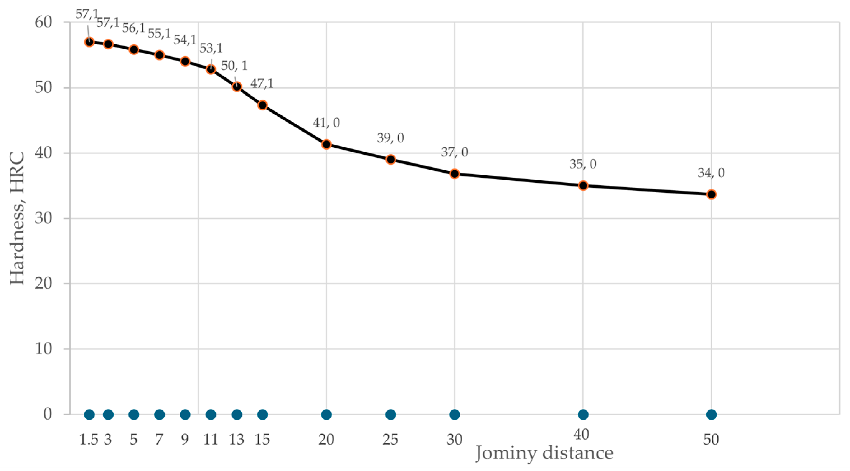
Figure 2.
Predictors of steel 42CrMo4 (hardnesses and microstructures).
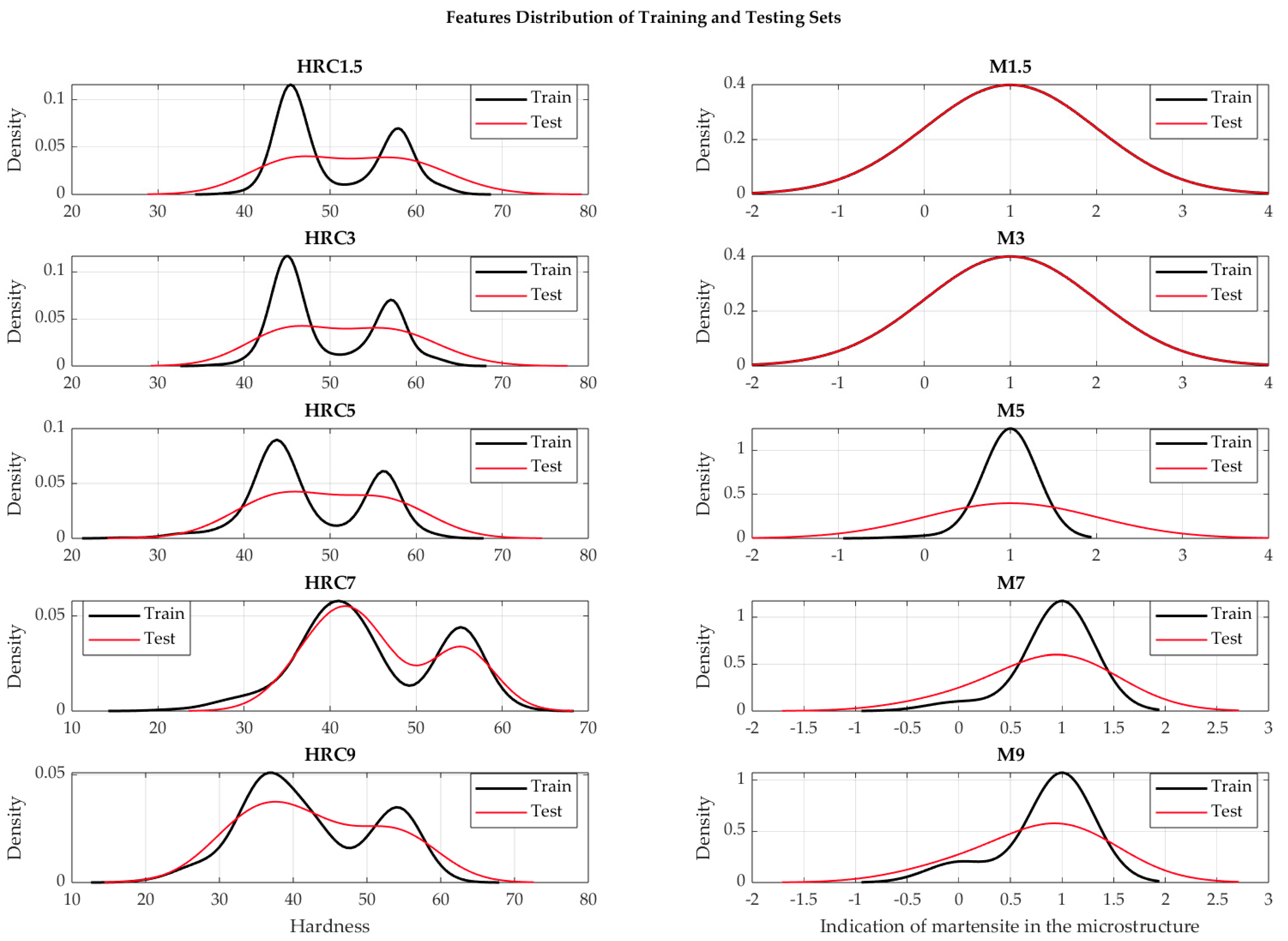
Figure 3.
Training and test dataset’s split distribution.
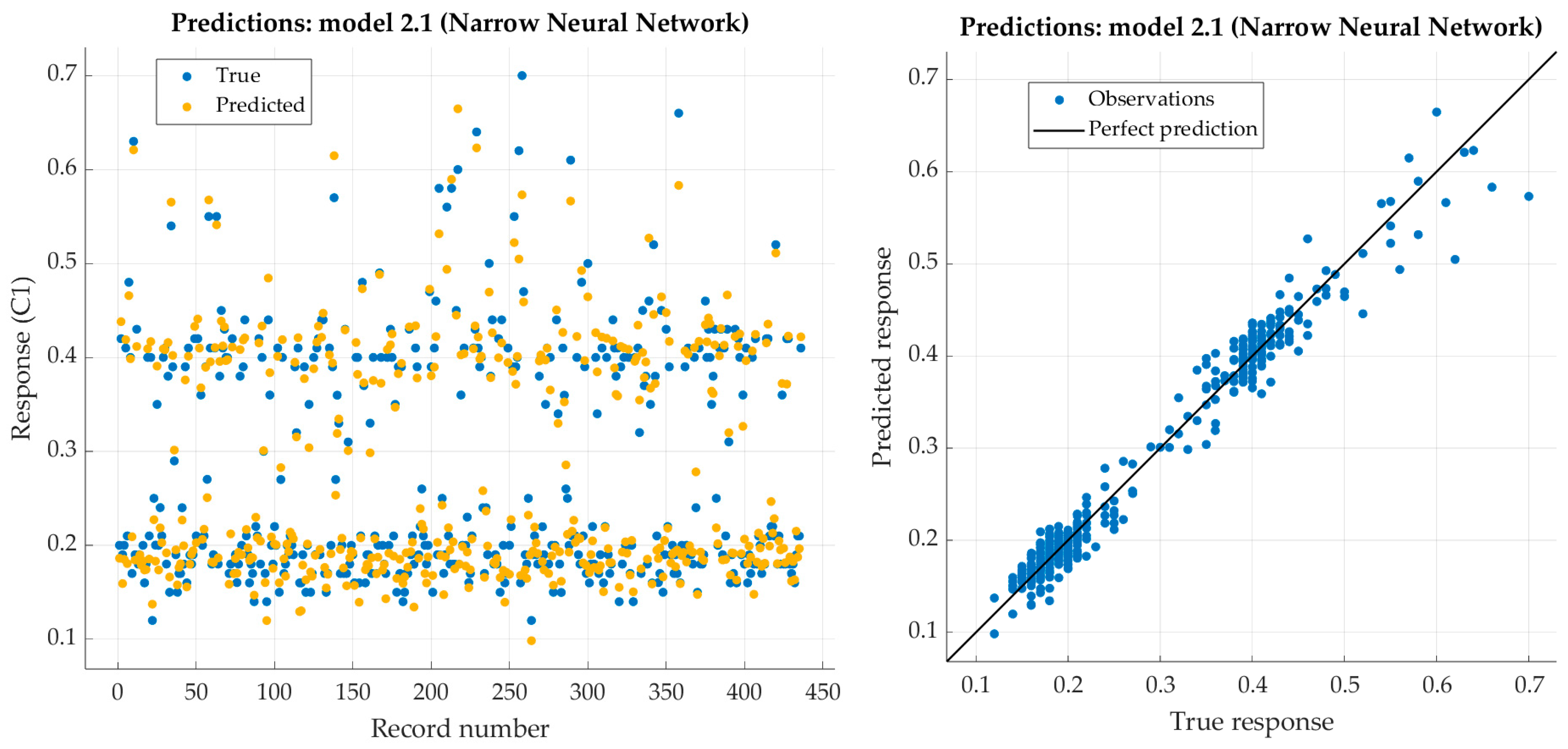
Figure 4.
Performance evaluation of narrow neural network on training dataset (carbon).
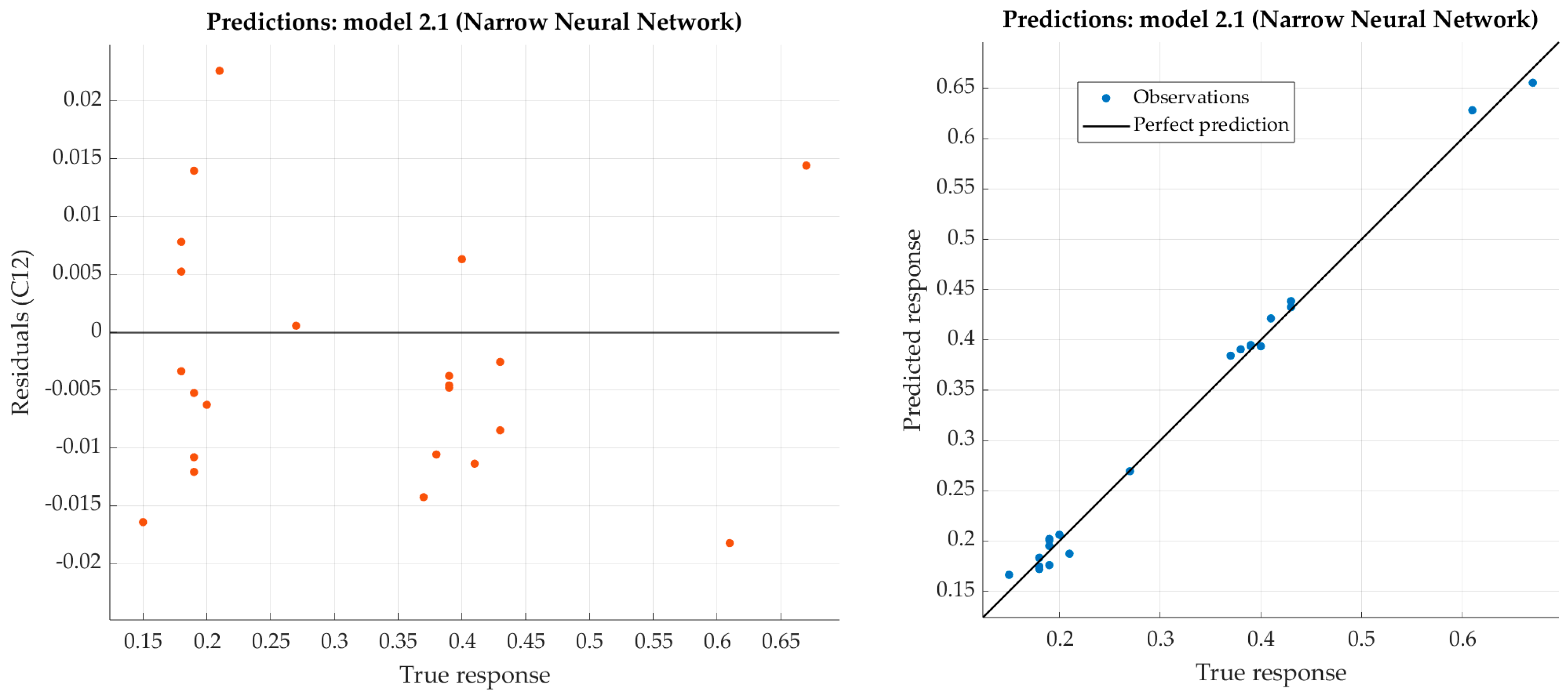
Figure 5.
Performance evaluation of narrow neural network on test dataset (carbon).
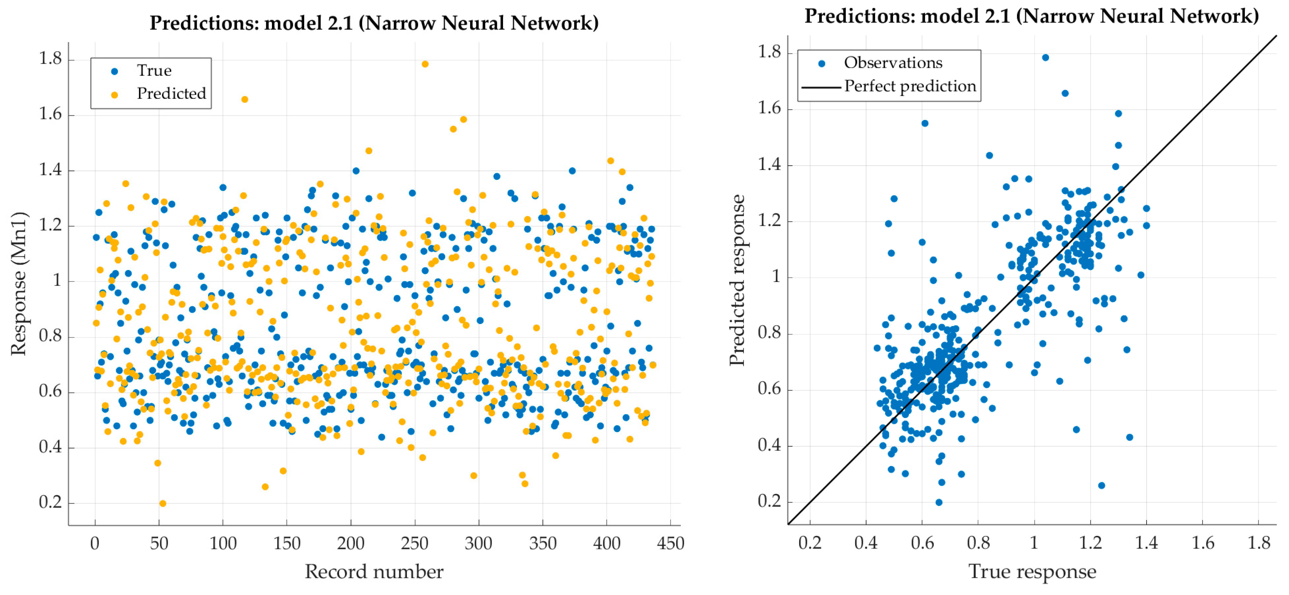
Figure 6.
Performance evaluation of narrow neural network on training dataset (manganese).
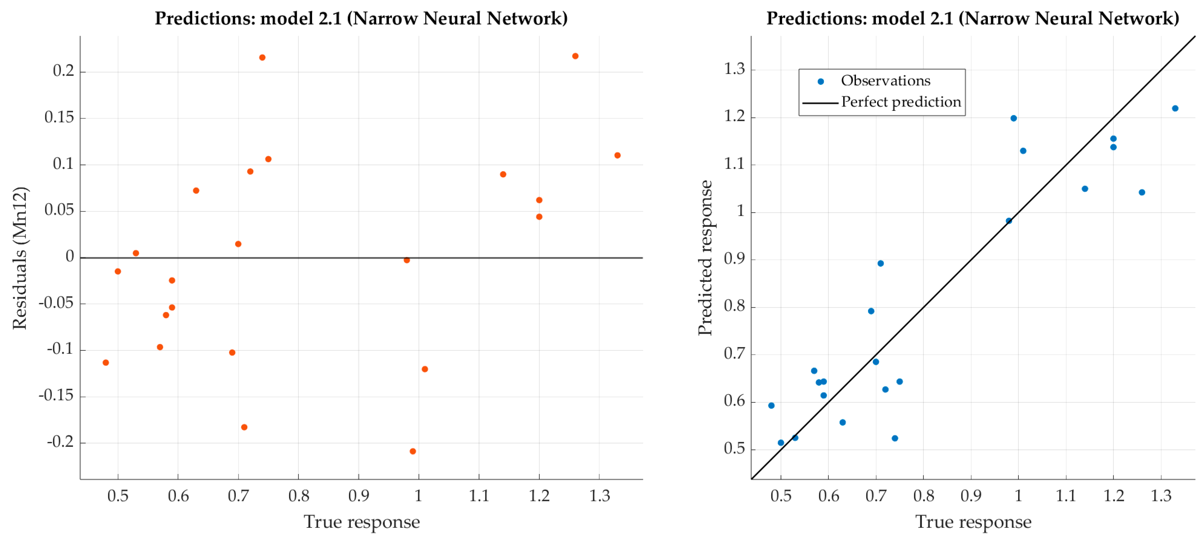
Figure 7.
Performance evaluation of narrow neural network on test dataset (manganese).
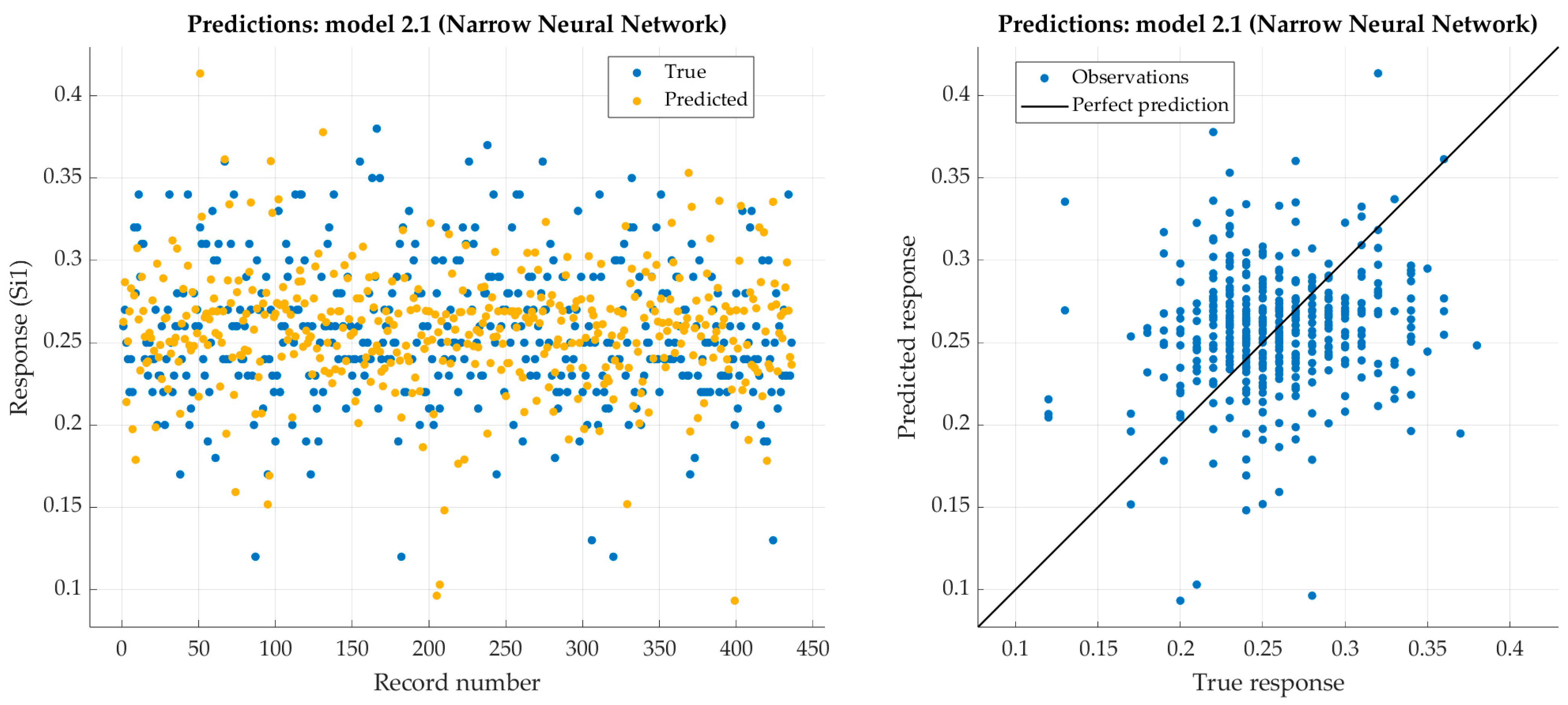
Figure 8.
Performance evaluation of narrow neural network on training dataset (silicon).
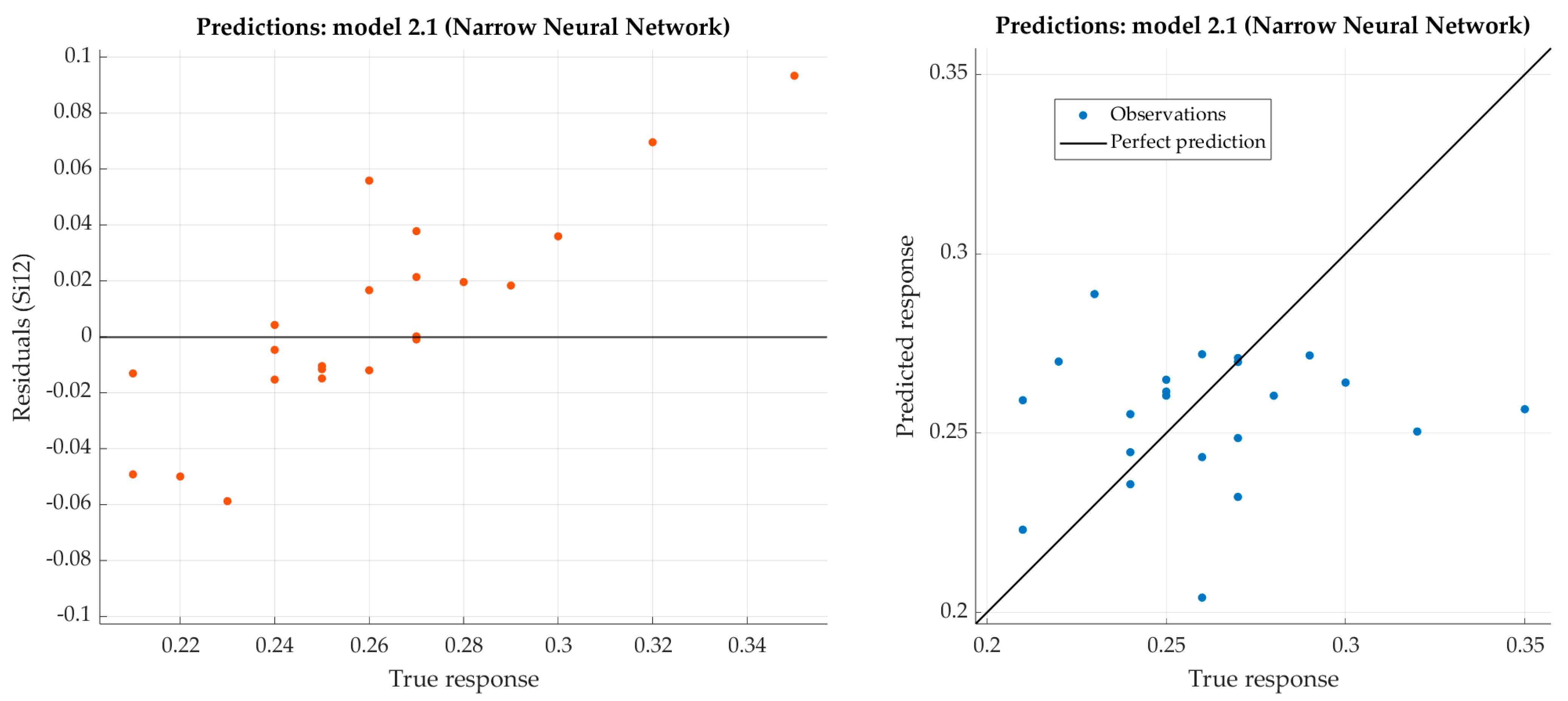
Figure 9.
Performance evaluation of narrow neural network on test dataset (silicon).
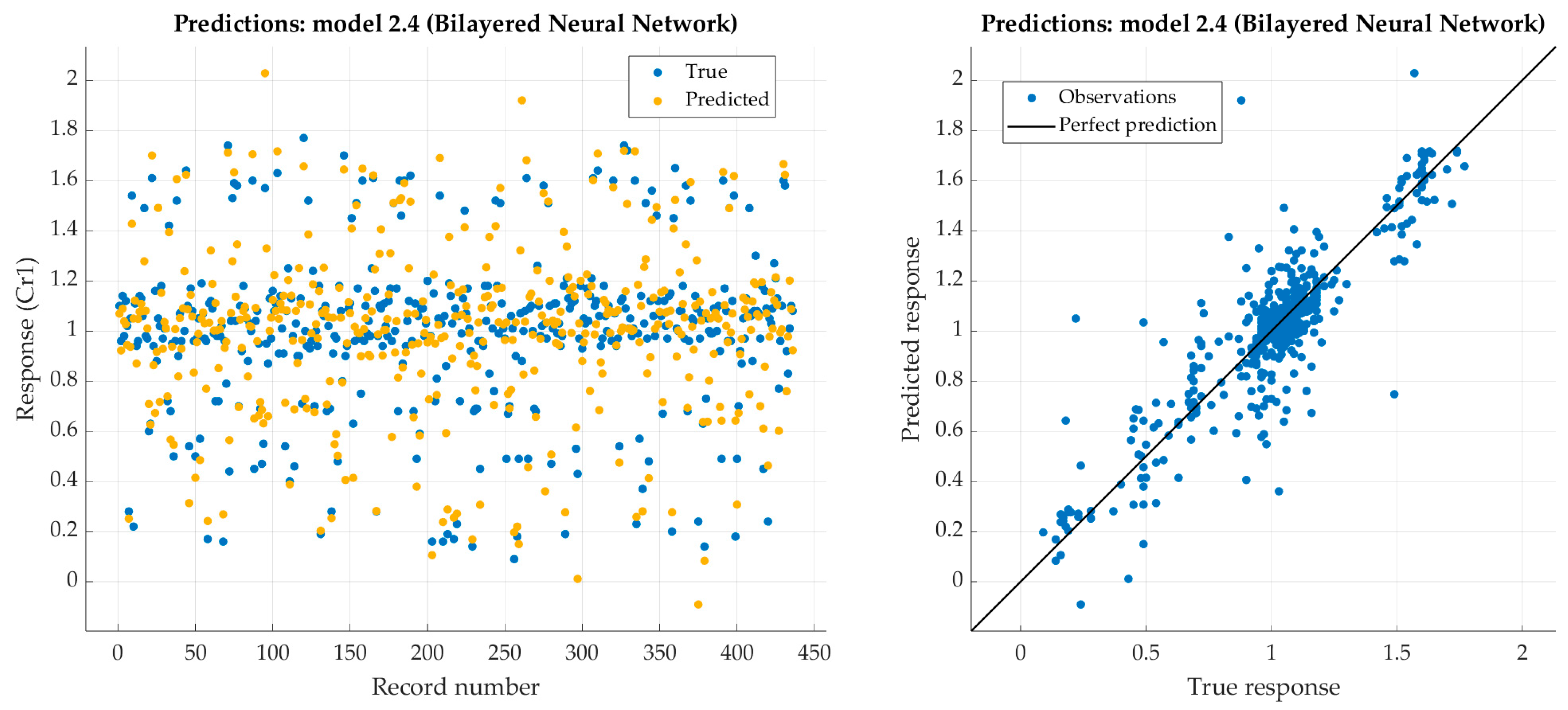
Figure 10.
Performance evaluation of bilayered neural network on training dataset (chromium).
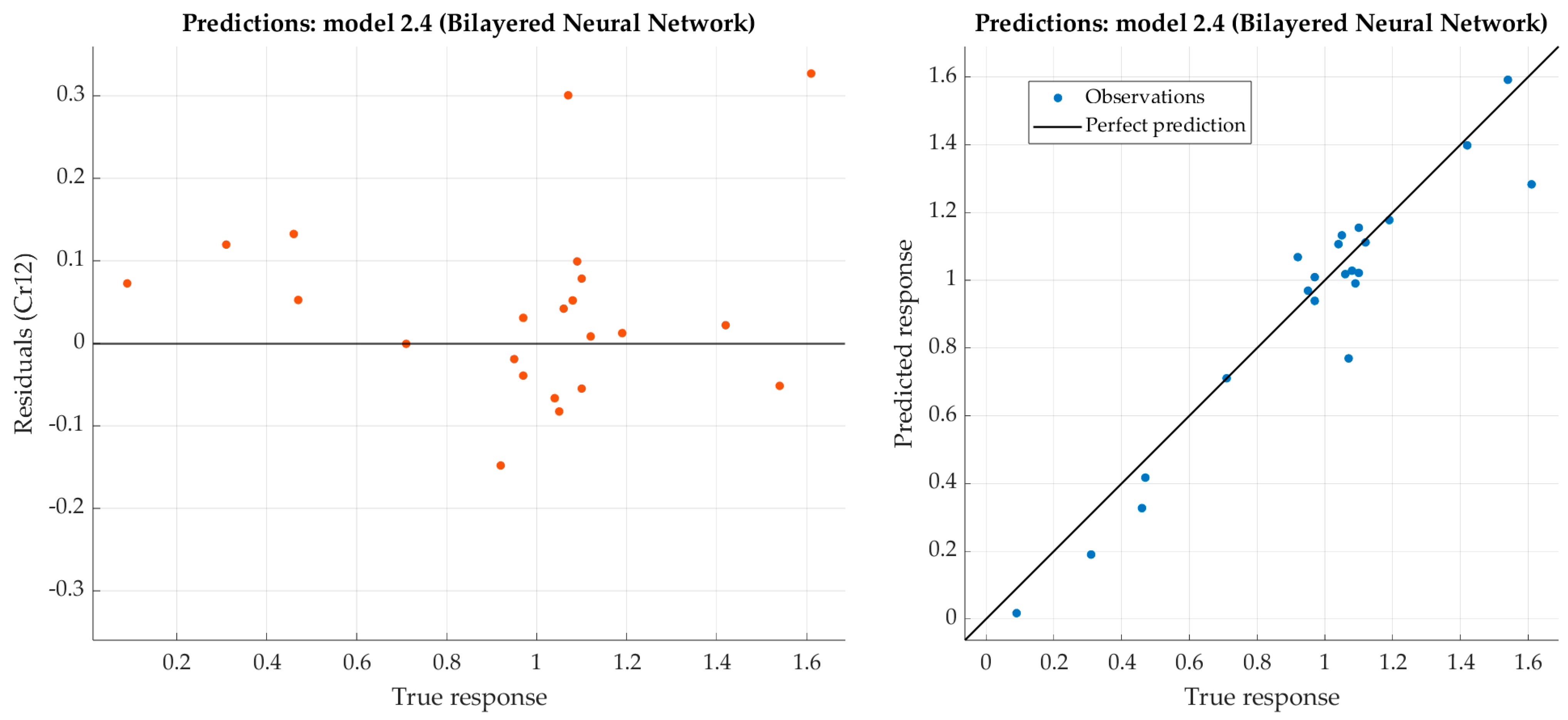
Figure 11.
Performance evaluation of bilayered narrow neural network on test dataset (chromium).
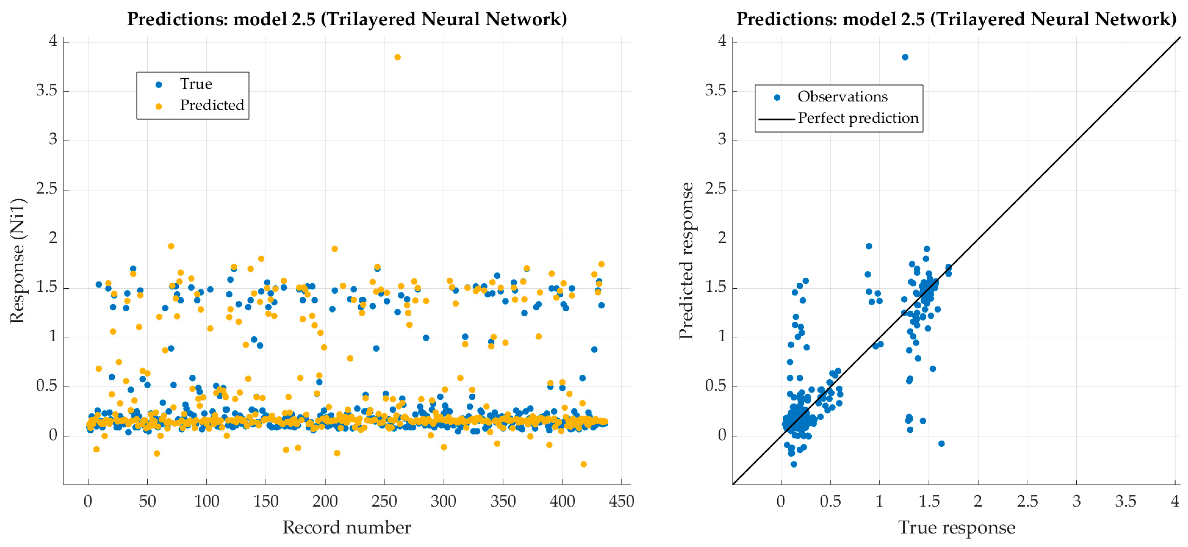
Figure 12.
Performance evaluation of trilayered neural network on training dataset (nickel).
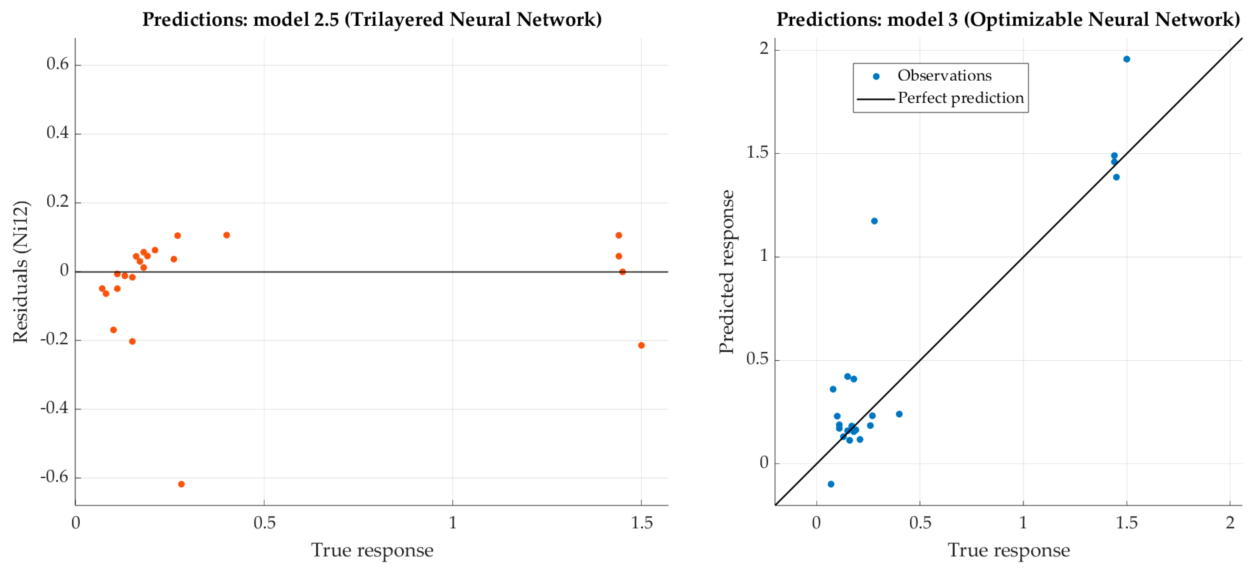
Figure 13.
Performance evaluation of trilayered narrow neural network on test dataset (nickel).
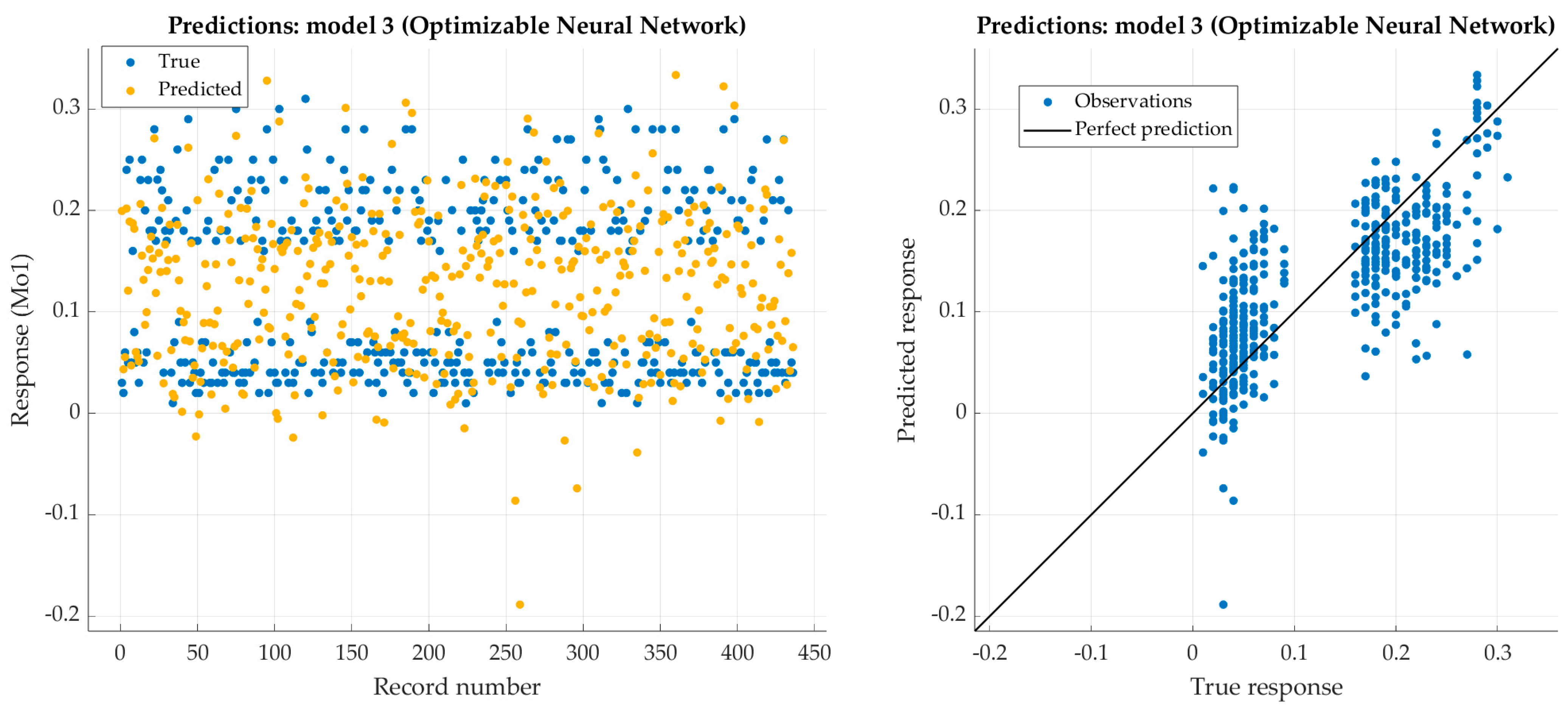
Figure 14.
Performance evaluation of optimized neural network on training dataset (molybdenum).
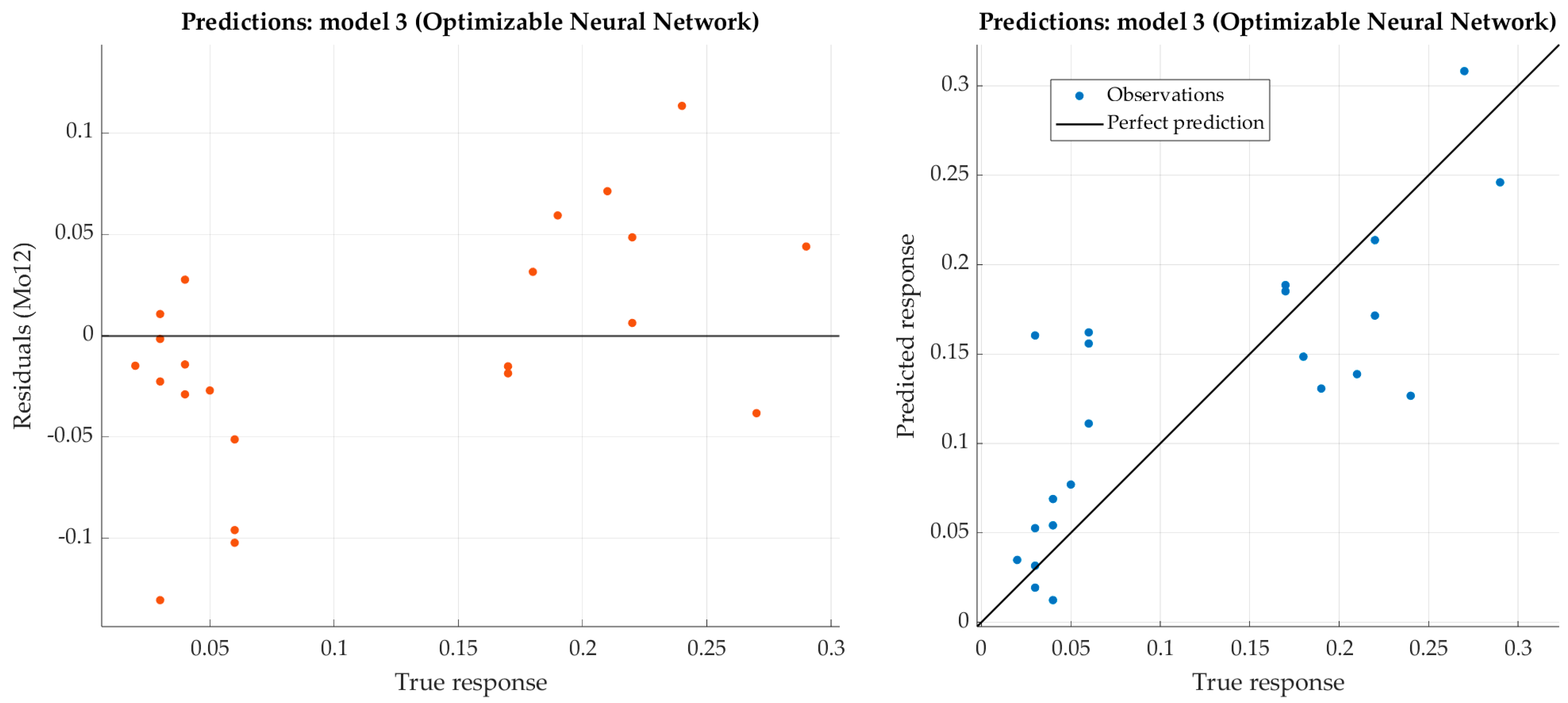
Figure 15.
Performance evaluation of optimized narrow neural network on test dataset (molybdenum).
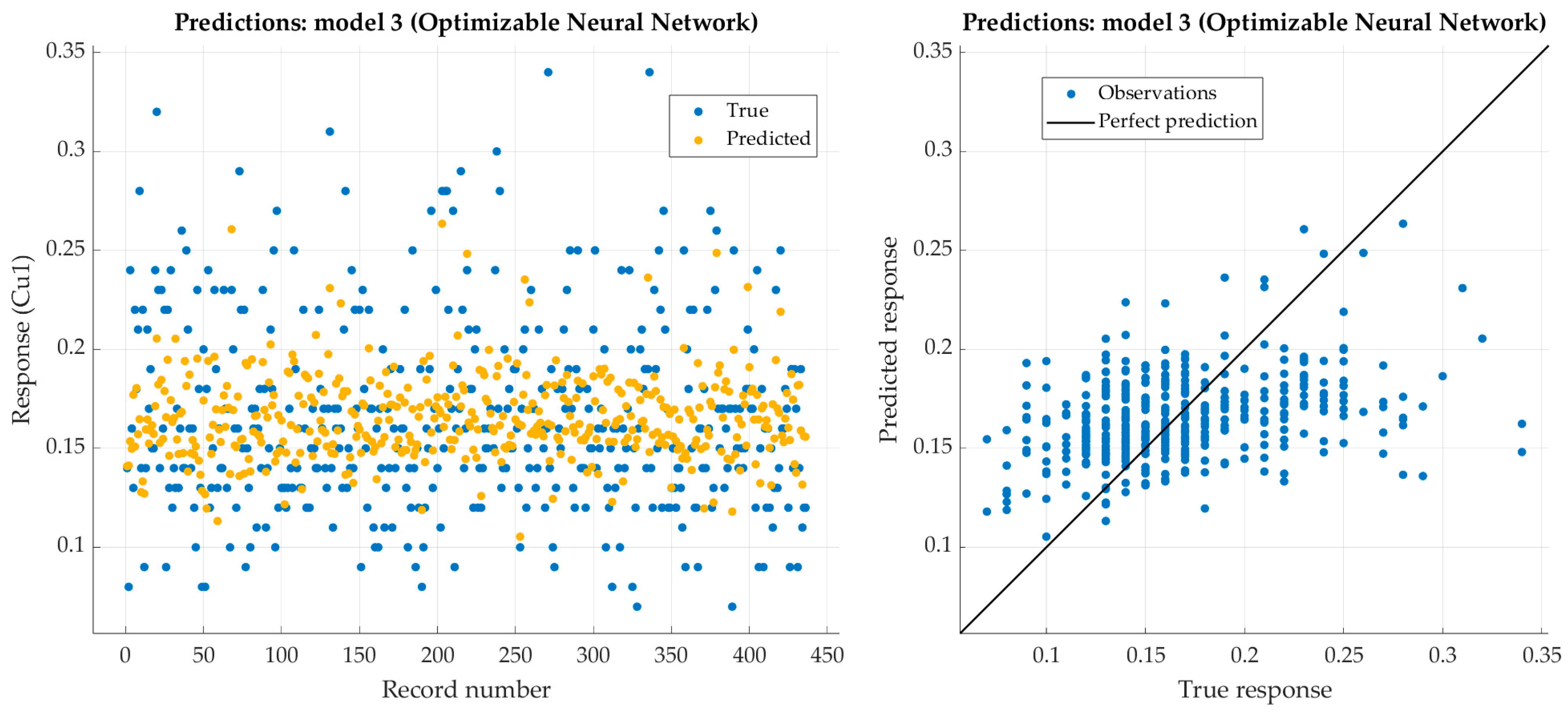
Figure 16.
Performance evaluation of narrow neural network on training dataset (copper).
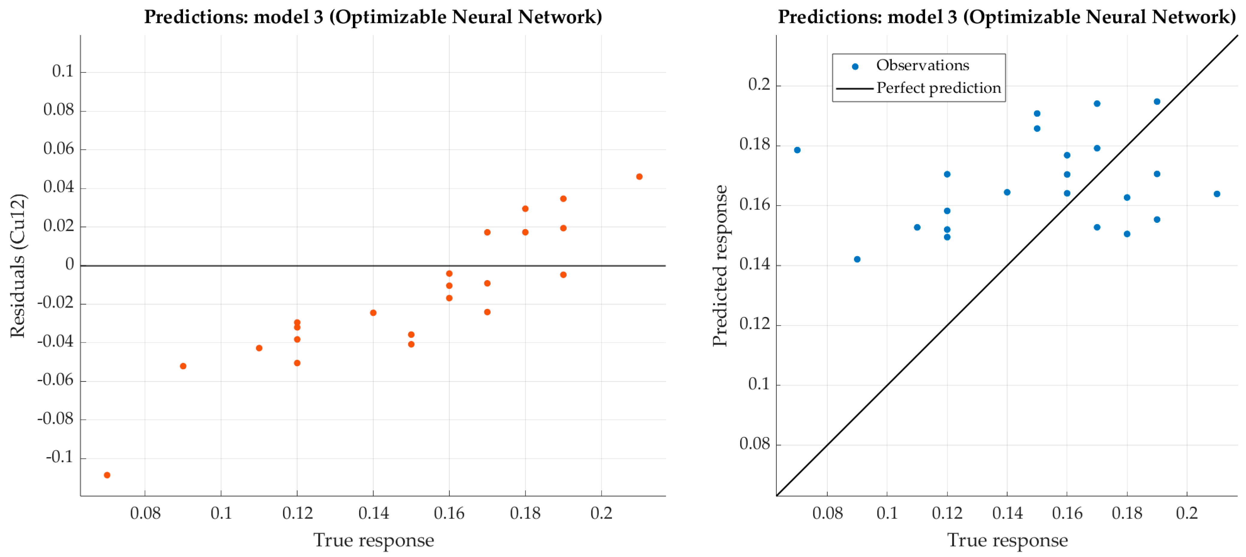
Figure 17.
Performance evaluation of optimized narrow neural network on test dataset (copper).
Table 1.
Ranges of predictor parameters (HRC) used to model chemical composition of steels.
| Hardness Range | HRC1.5 | HRC3 | HRC5 | HRC7 | HRC9 | HRC11 | HRC13 | HRC15 | HRC20 | HRC25 | HRC30 | HRC40 | HRC50 |
|---|
| Min. | 64.5 | 64 | 63 | 61 | 60 | 59.5 | 59 | 58 | 57 | 56 | 54 | 51 | 44 |
| Max. | 38.5 | 36.75 | 26 | 21.5 | 20.5 | 19 | 18 | 17 | 15 | 13 | 12 | 11 | 10 |
Table 2.
Predictors for one observation (steel 42CrMo4).
| M1.5 | M3 | M5 | M7 | M9 | M11 | M13 | M15 | M20 | M25 | M30 | M40 | M50 |
|---|
| 1 | 1 | 1 | 1 | 1 | 1 | 1 | 1 | 0 | 0 | 0 | 0 | 0 |
Table 3.
Responses for steel 42CrMo4 (chemical composition).
| C | Mn | Si | Cr | Ni | Mo | Cu |
|---|
| 0.4 | 0.7 | 0.2 | 1.01 | 0.16 | 0.16 | 0.2 |
Table 4.
Kolmogorov–Smirnov test results of goodness of fit of the training and test dataset.
| Features | HRC1.5 | HRC3 | HRC5 | HRC7 | HRC9 | HRC11 | HRC13 | HRC15 | HRC20 | HRC25 | HRC30 | HRC40 | HRC50 |
|---|
| KS-test value | 0.152 | 0.163 | 0.166 | 0.127 | 0.093 | 0.090 | 0.147 | 0.161 | 0.157 | 0.132 | 0.132 | 0.167 | 0.147 |
| p-value | 0.68 | 0.6 | 0.57 | 0.86 | 0.99 | 0.99 | 0.72 | 0.61 | 0.64 | 0.82 | 0.84 | 0.57 | 0.73 |
Table 5.
Kolmogorov–Smirnov test results of goodness of fit of the training and test dataset.
| Features | M1.5 | M3 | M5 | M7 | M9 | M11 | M13 | M15 | M20 | M25 | M30 | M40 | M50 |
|---|
| KS-test value | 0 | 0 | 0.018 | 0.106 | 0.071 | 0 | 0.001 | 0.037 | 0.031 | 0.027 | 0.044 | 0.037 | 0.009 |
| p-value | 1 | 1 | 1 | 0.96 | 1 | 1 | 1 | 1 | 1 | 1 | 1 | 1 | 1 |
Table 6.
Results after training for carbon with six different architectures of ANNs.
| Model | Architecture | RMSE | R2 | MAE | MSE |
|---|
| Train | Test | Train | Test | Test | Test |
|---|
| Narrow NN | 26-10-1 | 0.0204 | 0.0108 | 0.973 | 0.994 | 0.0093 | 0.0001 |
| Bilayered NN | 26-10-10-1 | 0.0191 | 0.0114 | 0.976 | 0.994 | 0.0085 | 0.0001 |
| Trilayered NN | 26-10-10-10-1 | 0.0218 | 0.0140 | 0.969 | 0.991 | 0.0111 | 0.0002 |
| Medium NN | 26-25-1 | 0.0200 | 0.0199 | 0.974 | 0.981 | 0.0137 | 0.0004 |
| Wide NN | 26-100-1 | 0.0292 | 0.0290 | 0.945 | 0.959 | 0.0164 | 0.0008 |
| Optimizable NN | 26-4-4-14-1 | 0.0232 | 0.0307 | 0.965 | 0.954 | 0.0202 | 0.0010 |
Table 7.
Results after training for manganese with six different architectures of ANNs.
| Model | Architecture | RMSE | R2 | MAE | MSE |
|---|
| Train | Test | Train | Test | Test | Test |
|---|
| Narrow NN | 26-10-1 | 0.1870 | 0.1122 | 0.485 | 0.823 | 0.0915 | 0.0126 |
| Trilayered NN | 26-10-10-10-1 | 0.1930 | 0.1163 | 0.451 | 0.810 | 0.0827 | 0.0135 |
| Wide NN | 26-100-1 | 0.2084 | 0.1251 | 0.361 | 0.780 | 0.0885 | 0.0157 |
| Optimizable NN | 26-3-1 | 0.1637 | 0.1362 | 0.605 | 0.739 | 0.1188 | 0.0186 |
| Medium NN | 26-25-1 | 0.2110 | 0.1665 | 0.344 | 0.610 | 0.1222 | 0.0277 |
| Bilayered NN | 26-10-10-1 | 0.2389 | 0.1918 | 0.160 | 0.482 | 0.1092 | 0.0368 |
Table 8.
Results after training for silicon with six different architectures of ANNs.
| Model | Architecture | RMSE | R2 | MAE | MSE |
|---|
| Train | Test | Train | Test | Test | Test |
|---|
| Optimizable NN | 26-5-1 | 0.0426 | 0.0342 | −0.011 | −0.072 | 0.0258 | 0.0012 |
| Narrow NN | 26-10-1 | 0.0515 | 0.0371 | −0.476 | −0.262 | 0.0279 | 0.0014 |
| Bilayered NN | 26-10-10-1 | 0.0645 | 0.0401 | −1.317 | −0.474 | 0.0317 | 0.0016 |
| Trilayered NN | 26-10-10-10-1 | 0.0717 | 0.0428 | −1.864 | −0.678 | 0.0333 | 0.0018 |
| Wide NN | 26-100-1 | 0.0757 | 0.0510 | −2.192 | −1.387 | 0.0392 | 0.0026 |
| Medium NN | 26-25-1 | 0.0622 | 0.0630 | −1.152 | −2.642 | 0.0405 | 0.0040 |
Table 9.
Results after training for chromium with six different architectures of ANNs.
| Model | Architecture | RMSE | R2 | MAE | MSE |
|---|
| Train | Test | Train | Test | Test | Test |
|---|
| Bilayered NN | 26-10-10-1 | 0.1609 | 0.1168 | 0.748 | 0.896 | 0.1047 | 0.0824 |
| Optimizable NN | 26-219-1 | 0.1308 | 0.1377 | 0.834 | 0.856 | 0.0939 | 0.0886 |
| Trilayered NN | 26-10-10-10-1 | 0.1518 | 0.1400 | 0.776 | 0.851 | 0.0963 | 0.1009 |
| Wide NN | 26-100-1 | 0.1539 | 0.1447 | 0.770 | 0.841 | 0.1033 | 0.0839 |
| Narrow NN | 26-10-1 | 0.1433 | 0.1748 | 0.800 | 0.767 | 0.1006 | 0.1310 |
| Medium NN | 26-25-1 | 0.1814 | 0.2039 | 0.680 | 0.684 | 0.1196 | 0.1304 |
Table 10.
Results after training for nickel with six different architectures of ANNs.
| Model | Architecture | RMSE | R2 | MAE | MSE |
|---|
| Train | Test | Train | Test | Test | Test |
|---|
| Trilayered NN | 26-10-10-10-1 | 0.2998 | 0.1590 | 0.660 | 0.899 | 0.0933 | 0.0253 |
| Bilayered NN | 26-10-10-1 | 0.3476 | 0.2386 | 0.544 | 0.771 | 0.1416 | 0.0569 |
| Optimizable NN | 26—1 | 0.2800 | 0.2450 | 0.704 | 0.759 | 0.1451 | 0.0600 |
| Wide NN | 26-100-1 | 0.3841 | 0.2715 | 0.443 | 0.704 | 0.1524 | 0.0737 |
| Narrow NN | 26-10-1 | 0.3537 | 0.3381 | 0.527 | 0.541 | 0.1986 | 0.1143 |
| Medium NN | 26-25-1 | 0.4303 | 0.3608 | 0.301 | 0.477 | 0.2241 | 0.1302 |
Table 11.
Results after training for molybdenum with six different architectures of ANNs.
| Model | Architecture | RMSE | R2 | MAE | MSE |
|---|
| Train | Test | Train | Test | Test | Test |
|---|
| Optimizable NN | 26-295-5-1 | 0.0611 | 0.0570 | 0.5160 | 0.613 | 0.0442 | 0.0033 |
| Trilayered NN | 26-10-10-10-1 | 0.0871 | 0.0634 | 0.0147 | 0.521 | 0.0417 | 0.0040 |
| Bilayered NN | 26-10-10-1 | 0.2185 | 0.0682 | −5.1983 | 0.445 | 0.0461 | 0.0047 |
| Narrow NN | 26-10-1 | 0.0798 | 0.0701 | 0.1732 | 0.415 | 0.0591 | 0.0049 |
| Wide NN | 26-100-1 | 0.1012 | 0.0832 | −0.3292 | 0.176 | 0.0558 | 0.0069 |
| Medium NN | 26-25-1 | 0.1009 | 0.1070 | −0.3205 | −0.364 | 0.0787 | 0.0115 |
Table 12.
Results after training for copper with six different architectures of ANNs.
| Model | Architecture | RMSE | R2 | MAE | MSE |
|---|
| Train | Test | Train | Test | Test | Test |
|---|
| Optimizable NN | 26-260-1 | 0.0442 | 0.0020 | 0.1505 | 0.0331 | 0.0297 | 0.0013 |
| Narrow NN | 26-10-1 | 0.0613 | 0.0038 | −0.6341 | 0.0452 | 0.0433 | 0.0036 |
| Medium NN | 26-25-1 | 0.0659 | 0.0043 | −0.8875 | 0.0462 | 0.0443 | 0.0042 |
| Trilayered NN | 26-10-10-10-1 | 0.0536 | 0.0029 | −0.2493 | 0.0394 | 0.0516 | 0.0049 |
| Wide NN | 26-100-1 | 0.0741 | 0.0055 | −1.3885 | 0.0500 | 0.0562 | 0.0052 |
| Bilayered NN | 26-10-10-1 | 0.0738 | 0.0055 | −1.3784 | 0.0457 | 0.0639 | 0.0098 |
Table 13.
Predicted vs. experimental data for content of chemical elements.
Chemical
Elements | | Steel Grades |
|---|
| | | C60E | 41Cr4 | 46Cr2 | 17CrNi6-6 | 17CrNi6-6 |
| C | Pred. vs. exp. values | 0.63 0.61 | 0.43 0.43 | 0.44 0.43 | 0.17 0.15 | 0.66 0.67 |
| Steel grade limits | 0.57–0.65 | 0.38 0.45 | 0.42–0.50 | 0.14–0.2 | 0.6–0.7 |
| Mn | Pred. vs. exp. values | 0.79 0.69 | 0.63 0.72 | 0.64 0.75 | 0.53 0.53 | 1.13 1.01 |
| Steel grade limits | 0.6–0.9 | 0.6–0.9 | 0.50–0.80 | 0.5–0.9 | 0.9–1.2 |
| Si | Pred. vs. exp. values | 0.26 0.24 | 0.27 0.27 | 0.20 0.26 | 0.27 0.22 | 0.25 0.32 |
| Steel grade limits | 0–0.4 | 0–0.4 | 0–0.40 | 0–0.4 | 0.25–0.50 |
| Cr | Pred. vs. exp. values | 0.19 0.31 | 0.99 1.09 | 0.42 0.47 | 1.4 1.42 | 0.02 0.09 |
| Steel grade limits | 0–0.4 | 0.9–1.2 | 0.4–0.6 | 1.4–1.7 | N/D |
| Ni | Pred. vs. exp. values | 0.12 0.11 | 0.17 0.15 | 0.29 0.40 | 1.45–1.45 | 0.12 0.07 |
| Steel grade limits | 0–0.4 | N/D * | N/D * | 1.4–1.7 | N/D * |
| Mo | Pred. vs. exp. values | 0.02 0.03 | 0.16 0.06 | 0.01 0.04 | 0.55 0.04 | 0.03 0.02 |
| Steel grade limits | 0–0.1 | N/D * | N/D * | N/D * | N/D * |
| Cu | Pred. vs. exp. values | 0.19 0.19 | 0.18 0.16 | 0.19 0.17 | 0.15 0.17 | 0.19 0.15 |
| Steel grade limits | N/D * | N/D * | N/D * | N/D * | N/D * |
| Disclaimer/Publisher’s Note: The statements, opinions and data contained in all publications are solely those of the individual author(s) and contributor(s) and not of MDPI and/or the editor(s). MDPI and/or the editor(s) disclaim responsibility for any injury to people or property resulting from any ideas, methods, instructions or products referred to in the content. |
© 2024 by the authors. Licensee MDPI, Basel, Switzerland. This article is an open access article distributed under the terms and conditions of the Creative Commons Attribution (CC BY) license (https://creativecommons.org/licenses/by/4.0/).


