Abstract
Leaf springs are components of railway rolling stock made of high-strength alloyed steel to resist loading and environmental conditions. Combining the geometric notches with the high surface roughness of its leaves, fatigue models based on local approaches might be more accurate than global ones. In this investigation, the monotonic and fatigue behaviour of 51CrV4 steel for application in leaf springs of railway rolling stock is analysed. Fatigue models based on strain-life and energy-life approaches are considered. Additionally, the transient and stabilised behaviours are analysed to evaluate the cyclic behaviour. Both cyclic elastoplastic and cyclic master curves are considered. Lastly, different fatigue fracture surfaces are analysed using SEM. As a result, the material properties and fatigue models can be applied further in either the design of leaf springs or in the mechanical designs of other components made of 51CrV4 steel.
1. Introduction
The industry offers a diverse range of spring steels with varying characteristics for several technical applications. Leaf springs for two-axle freight wagons are made of high-strength steel with high fatigue and corrosion strengths, including, for example, the 51CrV4 steel grade [1,2,3] (see Figure 1). In addition to being used for road and rail suspension vehicles, the 51CrV4 steel grade has been used in the design of industry machinery components such as gears, pinions, forged crankshafts, steering knuckles, connecting rods, spindles, pumps, and gear shafts [3,4,5]. Additionally, the characteristics of this steel grade have also been investigated for application in railway rails [6].
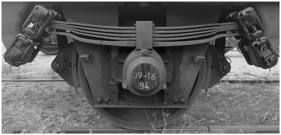
Figure 1.
Illustration of a parabolic leaf spring in a freight wagon suspension.
As a suspension component in cargo vehicles, for example, leaf springs are continuously subjected to dynamic loads, which increase the likelihood of failure due to fatigue phenomena. Since leaf springs are made of high-strength steel, these components usually exhibit a relatively high fatigue strength [7,8,9]; however, having notch geometries, the operating stresses are intensified, which might drastically reduce the fatigue resistance [10]. Besides, leaf springs have a high level of roughness, = 3.5 m [11], but can reach = 7 m (and maximum roughness, = 40 m) [12]; peak stress levels in the micro-notches above its yield strength can be generated, thus data collected in this study can be helpful for this type of analysis.
Examples of failures of these components have been reported. According to the literature, 70% of fatigue failures occurred in the middle section of the master leaf [13]. In some failures, the crack initiated in geometric notches. The observed remaining 30% of the failures appeared in areas (central and ends) where geometric details are often produced for leaf alignment [13,14,15,16,17]. Regarding the surface roughness effect, the fatigue failures observed in [18,19] prove its great detrimental effect on the resistance of these components.
Under these circumstances, fatigue models based on local elastoplastic analysis may be more suitable. Several researchers have performed local approaches based on strain-life fatigue resistance curves, such as the Coffin–Manson and Basquin (CMB), along with the cyclic elastoplastic mechanical model of the material in stabilised conditions, such as the Ramberg–Osgood (RO) model [20,21,22,23,24]. Since these leaves are subjected to the heat treatments of quenching and tempering to obtain the desired high mechanical strength, their strength may be compromised if the parameters of the tempering process are not well-calibrated. According to investigations carried out on martensitic steels [25], increasing the tempering temperature increases the amount of cyclic softening of the material and reduces the cyclic yield stress [26,27]. Additionally, in [25,27,28,29], it was also observed that increasing the tempering temperature from 300C reduces the fatigue resistance for medium and long lives, with a decrease in the coefficients and exponents of the CMB model.
In addition to the springs being developed only to absorb rail vibrations and maintain the contact between the vehicle and the rail, these components are responsible for supporting the wagon-container set. As a result, these components are constantly subjected to non-zero global mean stress and strain that depends on the weight of the wagon-container-goods set [15,30,31]. Thus, the CMB models fitted in terms of fully-reversed cyclic straining conditions should be corrected due to the presence of the mean stress effect. Despite the simplicity of this procedure, the mean stress effect correction is dependent on the method considered. Regarding the most common mean stress correction formulas, Smith–Watson–Topper (SWT) and Manson–Halford imply a mean stress effect that is equally detected by elastic and plastic strain amplitude components, whereas Glinka and Morrow ignore the mean stress effect in the plastic strain component [32]. Concerning the strain ratio effect on the fatigue life, the CMB models appear not to be affected by the strain ratio [33,34]; however, some references pointed out that the strain ratio may affect both the cyclic RO and CMB parameters in aluminium and steel alloys [34,35,36].
Despite strain-life fatigue models being widely used in engineering practices, their parameters have demonstrated sensitivity to the strain ratio effects. In contrast with strain-life models, energy-life models are less sensitive to the strain ratio effect [35]. Energy-based models may be used with either the cumulative plastic strain energy following the hysteresis energy model or the plastic strain energy per cycle, given a stabilised cycle [34,37,38]. In [25,27], it was also found that increasing the tempering temperature negatively affects the regression parameters of the models.
Given the highlighted concerns regarding the fatigue strength of 51CrV4 steel for leaf springs and the discrepancy in the assumptions of the prediction models taking into account the mean stress effect, both strain-life and energy-life fatigue models are considered in the analysis. Furthermore, an initial analysis of the mechanical properties under monotonic loading conditions and its comparison with the cyclic behaviour is also carried out in this research.
2. Cyclic Behaviour
Mechanical properties obtained via monotonic tests must be considered only for loading conditions that do not vary over time because, under cyclic conditions, significant differences in mechanical behaviour can be observed, namely in cyclic hysteresis loops. These changes are associated with phenomena such as cyclic hardening or softening, ratcheting, and mean stress relaxation, and can occur for up to 100% of the component’s life (until failure). Under cyclic straining conditions, steady-state hysteresis loops or quasi-stable hysteresis loops, as illustrated in Figure 2, are observed, such that the total strain range, , can be defined as
where is the stress range and is the strain range. The superscripts e and p denote the elastic and plastic parts of the strain.
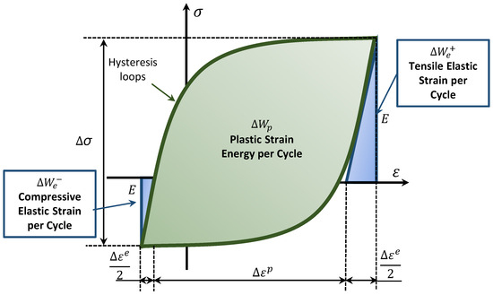
Figure 2.
Definition of a hysteresis loop, elastic energy in compression and tension, and plastic strain energy per cycle.
2.1. Cyclic Elastoplastic Behaviour
Materials presenting a symmetric stable hysteresis loop are called as Masing-type materials. Being Masing-type materials, the cyclic elastoplastic hardening curve is well-described by the RO relationship [39], such that
with denoting the range of strain or stress . E is the Young’s modulus, is the cyclic hardening strength coefficient, and is the cyclic strain hardening exponent. Several researchers still consider this power model in their fatigue life analysis, despite being an ancient model [40,41,42,43,44,45,46]. The parameters and may be determined via a linearised log–log regression analysis (more common) or, alternatively, via some curve fitting process, which is generally treated as a linear and nonlinear least-squares minimisation problem, respectively. The RO model can also be suitable under monotonic loading, such that the monotonic strength coefficient, K, and the monotonic strength exponent, n, are determined to be , where , and .
2.2. Master Curve Method
In the case of a material being considered a Masing-type material, the cyclic curve, written in Equation (2) and scaled by a factor of two, can be used to correctly describe the branches of the hysteresis loops [47]. Thus, an energetic relationship may be used to describe the fatigue behaviour of the material. It is assumed that, in the presence of a material exhibiting a Masing-type behaviour, the plastic strain energy per cycle, , may be related to the stress and strain amplitudes, such that
where is the elastoplastic hardening exponent given by Equation (2).
On the other hand, if the material exhibits a non-Masing behaviour, the cyclic curve obtained via Equation (2) does not generate suitable hysteresis loops. Instead of considering an Equation (2), the master curve method [48,49] must be considered and related to Equation (3), which is adjusted to take into account the non-Masing effect, such that [48,50,51]
where refers to the master curve’s cyclic parameters, and . Equation (4) relates the elastoplastic behaviour and the plastic strain energy per cycle, , for a non-Masing-type material, but can be also formulated in terms of RO parameters, and , according to the cyclic cumulative strain energy model presented by Ellyin for non-Masing materials [52] as
where is the increase in the proportional stress caused by the non-Masing behaviour.
3. Fatigue Life Prediction
3.1. Strain-Based Life Method
In the presence of plastic deformations, the fatigue strain-based models such as the CMB are suitable [53,54,55]. The CMB model relates the number of reversals to failure, , with the total strain amplitude, , via Equation (6), such that
where is the fatigue strength coefficient, is the fatigue ductility coefficient, is the fatigue strength exponent, and is the fatigue ductility exponent. The determination of the coefficients and exponents is made considering the pseudo-stabilised hysteresis loops. The transition point at which both elastic and plastic strain components have the same weight for fatigue is given by the intersection of the elastic and plastic terms of the Equation (6).
3.2. Total Energy Density-Life Method
Fatigue prediction methods based on the strain energy density parameter provide some advantages compared with the strain-life method [35]. In energy-based methods, the plastic strain energy per cycle, , is assumed to be the main contribution to the material fatigue damage process. Since remains almost constant throughout life [56,57], is related to the number of reversals to failure, , such that [56]
where and are empirically determined parameters. Equation (7) is extended to the high-cycle regime, considering the total strain energy, , as a fatigue parameter instead. is defined as the sum of the hysteresis energy and the elastic energy associated with the tensile stress per cycle, [58]. The fatigue predictions are still improved by introducing into the energy model the residual fatigue resistance, , which denotes the tensile elastic energy associated with the material fatigue limit. Thus, Equation (7) is rewritten in terms of the total strain energy as
where the parameters and are also determined experimentally. The parameter has been shown to be almost independent of the strain ratio at a constant strain amplitude and suitable for fully-reversed and non-null mean stress conditions [35,59].
4. Material and Procedures for Experimental and Statistical Analysis
4.1. Chemical Composition and Microstructure
The steel under investigation is the chromium-vanadium alloyed steel 51CrV4 with an average carbon content of roughly 0.50%, as presented in Table 1. Being quenched at 850 °C (40 min) in an oil bath and then tempered at 450 °C for 90 min, the 51CrV4 steel exhibits a tempered martensite microstructure with retained austenite (white phases), as shown in Figure 3.

Table 1.
Standard chemical composition of 51CrV4 steel grade in % wt.
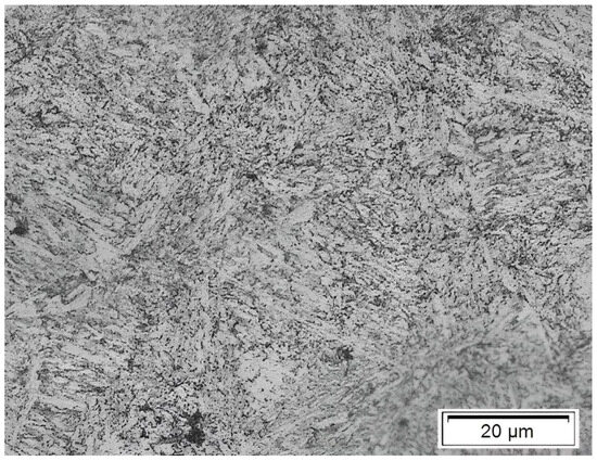
Figure 3.
Representation of an optical micro-graph for the chromium-vanadium alloyed steel at a tempering temperature of 450C, for 90 min.
4.2. Monotonic and Cyclic Tests
Monotonic tensile tests of the tempered 51CrV4 steel with a Vickers hardness of 447.65 HV were conducted at room temperature, according to the EN NP 10002-1 [60] or ISO 6892-1 [61] standards. An MTS 810 testing machine equipped with a load cell with ±100 kN capacity, a digital controller MTS FlexTest 40, and an MTS clip strain gauge with a 50 mm gauge length, calibrated from −10% up to 50%, were used to carry out the experimental tests at a displacement rate of 1.0 mm/min. Twenty samples from distinct batches of leaves were manufactured with an 8.02 ± 0.13 mm gauge diameter and 60 mm long cylindrical uniform-gauge length, as depicted in Figure 4A). Table 2 summarises the dimensions of the samples. In addition, Young’s modulus was determined via the experimental method described in ASTM E111-04 [62].
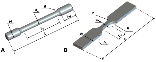
Figure 4.
Geometry of the specimens used in (A) monotonic tests and (B) fatigue tests.
Table 2.
Average dimensions of specimens used in monotonic tensile tests in accordance with EN NP 10002-1 standard [60] or ISO 6892-1 standard [61].
Regarding fatigue testing samples, a set of seven samples, also from distinct batches of leaves, were machined in flat-sheet shape specimens according to ASTM E606 standard [63]. Specimens had a net cross-section of = 38.98 ± 0.28 mm2 whose width, , is mm and thickness, , is mm (see Figure 4B). Table 3 presents the dimensions of the samples.
Table 3.
Geometry statistics of low-cycle fatigue specimen and general testing parameters.
With respect to the fatigue setup, cyclic tests were conducted under uniaxial strain-controlled conditions in an INSTRON 8801 servo-hydraulic machine (ServoHydraulic, Lingen (Ems), Germany) with a load cell of 100 kN, with a dynamic INSTRON 2620-202 (Instron®, Norwood, MA, USA) clip gauge with a working range of ±2.5 mm. The constant-step method scheme with a sinusoidal waveform function with a constant strain ratio of was considered. Fatigue tests were carried out at strain amplitudes of 0.375%, 0.50%, 0.75%, 1.00%, and 1.25% with repetitions for strain levels 0.375% and 0.50%. All specimens were tested at a constant average strain rate, .
4.3. Statistical Techniques
The cyclic behaviour and fatigue life prediction models presented in this paper are usually calibrated using linear regression methods, whose parameters are estimated via the ordinary least-squares method [64], as suggested by the ASTM E739-9 standard [65]. Thus, the linear response function may be written as
with and denoting, respectively, the vector of dependent and independent variables. The estimators and are determined as follows:
and
where and denote the sample average values for dependent and independent variables and , respectively. For the case of prediction curves described by a power law, the logarithm is applied to the random variables.
5. Results and Discussion
5.1. Mechanical Properties
The Young’s modulus, E, was determined considering the straight-line method, taking the coefficient of variation, , as a control parameter for the convergence process [66]. The convergence process is illustrated in Figure 5, showing that the achieved minimum value for was less than 2%. Applying this method in the 20 experimental results with a value of E = 200.54 ± 6.02 GPa, this method identifies a proportional limit stress, , for the 51CrV4 of 1030.51 ± 85.66 MPa.
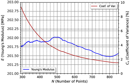
Figure 5.
Illustration of optimisation procedure in order to obtain the optimal value of longitudinal elasticity modulus, considering the maximum points for the linear regression model.
Monotonic tensile tests were performed until fracture, resulting in the evolution of the monotonic strength curves presented in Figure 6. Comparing the mechanical behaviour of four specimens (from the same batch) manufactured in the longitudinal (three samples) and transversal (one sample) directions, one verifies that the 51CrV4 steel grade is isotropic both in the elastic and plastic regimes with low scatter. However, considering the data gathered from 20 specimens (different batches), a large scatter is observed from the box plots (green boxes), with a yield strength at 0.2% of the residual plastic strain, , of 1271.48 ± 53.32 MPa, and with an ultimate tensile strength, , of 1438.35 ± 73.84 MPa, with a minimum and maximum of 1400.72 and 1601.62 MPa, respectively. Despite the large scatter, the analysed material is following the standardised values for 51CrV4 shown in Table 4, with denoting the strain level corresponding to , and the strain at fracture measured via the MTS contact strain gauge.
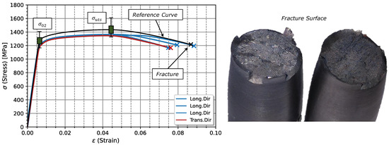
Figure 6.
Analysis of the engineering monotonic mechanical behaviour of the 51CrV4 steel grade: isotropy and fracture surfaces under monotonic tensile testing conditions.
Table 4.
Mechanical properties obtained from monotonic tensile tests for the chromium-vanadium alloyed steel.
Regarding the fracture surfaces observed for all tested specimens, Figure 6—right represents the most common fracture surface observed. According to this reference fracture surface, it is noted that, under monotonic loading conditions, the 51CrV4 steel has a semi-brittle macroscopic fracture, with an interior fracture mainly via the cleavage and a shear zone at 45C in relation to the plane containing the fracture surface in the outside region. This fracture is expected since 51CrV4 only exhibits a reduction area at fracture, , of mm (corresponding to a true strain level at fracture, , of %). Although the macroscopically fractured surfaces have a brittle appearance, mixed modes of cleavage and ductile-dimples were observed [67].
5.2. Cyclic Softening and Relaxation
Cyclic tests were carried out until failure; however, cyclic parameters are determined by considering the criterion of 50% of the total life. Figure 7 depicts the comparison between the hysteresis stress-strain loops at the first cycle and the cycle corresponding to the half-life. According to Figure 7, distinct levels of stress softening and mean stress relaxation were observed.
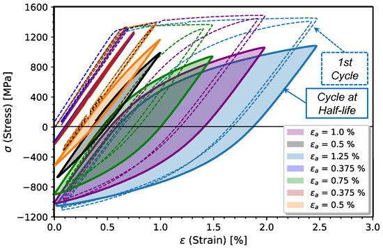
Figure 7.
51CrV4 steel behaviour under cyclic straining conditions for 1st cycle (dashed lines) and cycle corresponding to the half-life (continuous lines).
Figure 8 and Figure 9 present the evolution of the stress amplitude and mean stress throughout the cyclic test. Notice that there was a delay in the first phase of the cyclic test to reach the desired strain range, around 10 cycles; however, this will not affect the global cyclic behaviour. Analysing the evolution of the stress amplitude and mean stress throughout the cyclic test as presented in Figure 8 and Figure 9, one verifies that for the highest strain amplitudes, from up to , stress softening along with mean stress relaxation is always observed. However, for lower strain levels, up to , a slight stress hardening with no significant relaxation of mean stress is observed. In accordance with these observations, there will be a transition strain value that induces a significant mean stress relaxation. Observing Figure 9, the strain level might be 0.50%.
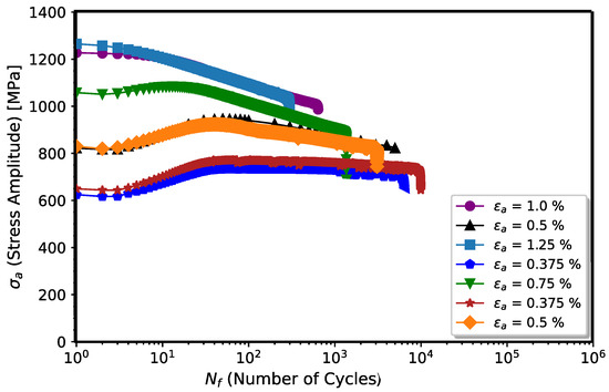
Figure 8.
Evolution of the stress amplitude throughout the cyclic test.
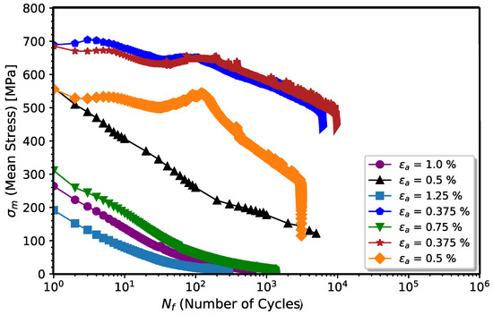
Figure 9.
Evolution of the mean stress throughout the cyclic test.
Since the phenomena of softening and relaxation are dependent on the applied total strain, a relationship can be considered to predict the stress level in stabilised or pseudo-stabilised conditions. Therefore, considering that the softening and cyclic relaxation occur only for non-null plastic strain conditions, a power law (Equation (12)) is assumed to be fitted to the cyclic softening stress amplitude and mean stress relaxation, with the plastic strain amplitude at the first cycle, , such that
with index k equalling m or a if we are determining the mean stress or stress amplitude variation. and denote, respectively, the stress amplitude and mean stress for half-life.
Figure 10 depicts the power law fitted to the stress amplitude and mean stress relationships. The coefficient and exponent regressors are computed by using the regression model in Equation (9), resulting in = 0.7009 and = −0.0376 (for the stress amplitude softening curve) and = 0.0041 and = −0.5760 (for the mean stress relaxation curve). Both models showed an adequate fit with the coefficient of determinations, , respectively, of 0.8740 and 0.8201. In accordance with Equation (12), for the corresponding plastic strain amplitude at fracture and for strain ratio, = 0, the result is a stress amplitude softening ratio of = 0.7433 and mean stress relaxation ratio of = 0.0101.
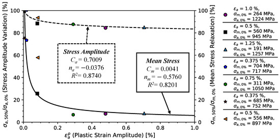
Figure 10.
Variation of the cyclic mean stress and stress amplitude with the applied plastic strain amplitude. Ratio between stress at the first cycle and the cycle corresponding to the half-life.
5.3. Monotonic and Cyclic Curves
The elastoplastic curve in the stabilised cyclic conditions is modeled by the RO model presented in Equation (2). The parameters and are obtained by using the least-squares method (Equation (9)) with the plastic term of Equation (2) linearised, considering all hysteresis loops centered in the origin. Figure 11 illustrates the comparison between stable hysteresis loops for the monotonic and RO models. According to the coefficient of determination determined from the RO cyclic model (black continuous line), a good fitting ( = 0.8236) between the RO cyclic model ( MPa and = 0.0790) and the stabilised hysteresis loops was obtained. Comparing the RO cyclic model with the RO model under monotonic conditions, a reduction from (monotonic) to MPa (cyclic) and an increase from to is observed. Concerning the cyclic yield strength, the cyclic stress is 836.97 MPa. Under cyclic conditions, 0.2% of the residual plastic strain is usually too high of a value, therefore the cyclic stress for 0.01% of the residual plastic strain tends to provide a better adjustment [68]. This value is often named the cyclic proportional limit, , since the residual plastic strain level is very low. Our analysis found a value for the cyclic proportional limit, , of 628.92 MPa (42.26% less than ). Table 5 summarises the comparison of the cyclic and monotonic properties obtained from the Ramberg–Osgood model.
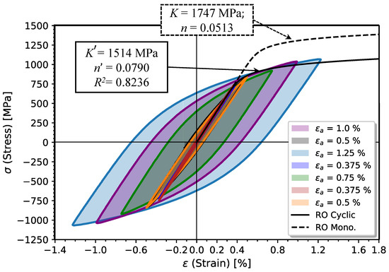
Figure 11.
Representation of the stable hysteresis loops obtained from cyclic tests. Comparison of the elastoplastic hardening model obtained from cyclic conditions with the monotonic elastoplastic curve.
Table 5.
Elastoplastic parameters for monotonic and cyclic loading conditions considering the Ramberg–Osgood model for 51CrV4 steel grade.
Since the cyclic RO parameters are obtained for , it is appropriate to compare them with the coefficient and the exponent estimated from monotonic tensile properties. Thus, considering the regressions with the highest in [69], such that
and
results in MPa, , and MPa. Comparing the estimated , , and with the ones obtained from the experiments, one verifies that there is no significant variation in the K (3.70%); however, there is an increase in , from 0.0790 to 0.1083 (37.09%). Regarding the cyclic stress, , a slight decrease of 1.99% is observed (from 836.97 to 820.28 MPa). Considering the highest difference in associated with the regression scatter analysed in [69], one verifies that and tend to remain with .
5.4. Master Curve
In order to verify if the 51CrV4 material exhibits a Masing-type behaviour, the hysteresis loops are superimposed as shown in Figure 12. Analysing the upper branches of the hysteresis loops, one verifies that the material does not exhibit ideal Masing-type behaviour, and therefore the master curve method is considered. From the linearised least-squares method results, the coefficient = 2414.71 MPa and exponent = 0.1250, with . Table 5 presents the parameters determined for the master curve and the comparison with the cyclic curve parameters.
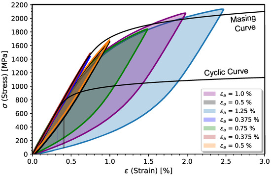
Figure 12.
Verification of the Masing-type behaviour and the cyclic curve for the 51CrV4 steel.
The determination of the coefficient and exponent of the master curve is made using the linear regression model. The linear regression model gives MPa and with a coefficient of determination . Notice that if only the data with quasi-full mean stress relaxation are considered, then and increase to 2638.33 MPa and 0.1614, respectively. Figure 13 depicts the fit of the master curve to all strain ranges tested. Notice that hysteresis loops are fitted for positive values of . The non-Masing behaviour has been verified for high-strength steels with low ductility [47,70]. On the other hand, the negative values of have been noted for steels with a lower strength [58]. As the value of is related to the level of non-Masing behaviour, from Figure 13, a high level of non-Masing-type behaviour for steel 51CrV4 for the lowest strain amplitudes (especially for a strain amplitude of 0.375%.) is verified. Table 5 presents the parameters determined for the master curve and the comparison with the cyclic curve parameters.
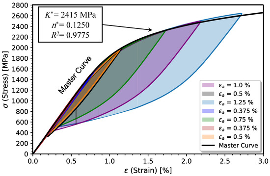
Figure 13.
Representation of the master curve after adjusting the upper branches of the stable hysteresis loops.
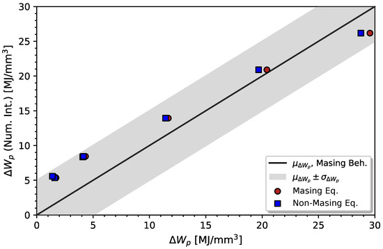
Evaluating the obtained results by comparing the plastic strain energy per cycle computed from Equations (3) and (4), and via the direct numerical integration of each hysteresis loop, it is possible to obtain a comparison as presented in Figure 14. The numerical integration method of each hysteresis loop is described by , with l and u denoting the loading and unloading process. For both the loading and unloading process, the numerical integral is given by . Comparing the numerical method with the obtained values of Equations (3) and (4), one verifies that the maximum variation occurs for the lowest strain amplitudes. However, all points in the analysis are within a deviation range of ±34.1%. As aforementioned, the specimens have a slight difference in monotonic behaviour (see Figure 6), and, therefore, some deviation from the ideal Masing-type behaviour might also be a result of this scatter.
5.5. Strain-Life Behaviour
The fatigue life curve under strain-controlled conditions is modelled considering the CMB model (Equation (6)). Applying the respective logarithmic transformations to and , with the index i denoting the respective data point and the index j the respective elastic term, e, or plastic, p, results in MPa, , , and (see Table 6). According to the coefficients of determination for the Coffin–Manson and Basquin models, a good fit was achieved ( = 0.9541 and , respectively). Figure 15 graphically depicts the CMB model (in green) and the respective curves of Basquin (in red), and Coffin–Manson (in blue). Regarding the number of reversals for the transition behaviour from monotonic to fatigue fractures, , 13 reversals were observed, which indicates a slight deviation from the prediction model. Moving to the transition point, reversals were found. After this transition point, the plastic strain decreases rapidly until the fatigue process starts to be totally governed by the elastic component ( = 1.80 reversals) for a residual plastic strain of 0.01%.
Table 6.
Parameters of Coffin–Manson and Basquin (6) obtained from linear regression.
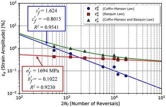
Figure 15.
Strain-life fatigue behaviour of 51CrV4 considering the Coffin–Manson and Basquin power laws.
Regarding the coefficients of the regression, and , both are often assumed to be of the same order of magnitude of and , respectively. In contrast with , is at least 20 times higher than . Considering the estimation models for strain-life parameters based on monotonic properties, one verifies that, from the Modified Universal Slopes method, MUSM [71], MPa (higher 17.69%), and (lower 594.2%), with the exponents and being constants, −0.09 (higher 13.56%) and −0.56 (higher 43.13%), respectively. If the Modified Four-point method, MFPM [72], is considered, the same coefficients are inferior; MPa (9.49% lower), (281.2% lower), and the exponents and are, respectively, (46.28% higher) and (44.99% higher). The same trend is verified when the median model, MM [73], is considered: MPa (21.52% higher), (260.9% lower), , and .
Comparison with the 51CrV4 steel obtained by tempering at a temperature of 540–650C in [6] ( = 1601.15 MPa, = 0.4780, = −0.093, and = −0.684), the model predicts that for a lower tempering temperature of 450C (as in the case of the steel investigated in this article), the fatigue resistance is higher for 100 reversals (), approximately; that is, LCF + HCF. On the other hand, 51CrV4 steel in [6] will tend to have greater resistance for lives of less than 100 reversals.
From the comparison of the results obtained with the estimated models, the strain ratio effect (mean stress effect) on the fatigue properties of the CMB model is clear. Although the fatigue data fits well with the CMB model, the fatigue properties obtained by the regression are not usually considered by other models (SWT [32], GSA [74], etc.). Thus, considering fatigue data corresponding only to loads where the cyclic relaxation effect is strongly observed (), using the linear regression method results in MPa, , , and , with and , respectively. Considering only this data set, the fatigue parameters obtained are now closer to the MUSM model, with a difference of 23.91% for , 0.83% for , 2.11% for , and 5.68% for . Comparing with the fatigue parameters initially obtained in this investigation, it is verified that the plastic terms, and , were more affected by than the elastic terms, and . Table 6 presents the summary of the analysis for the fatigue strength curve.
In [75], the same load ratio tests were carried out for two structural steels (a mild-strength steel and a high-strength steel) and a hot work tool steel. As expected, the higher-strength steels obtained a higher value of coefficients and exponents compared with the lower-strength steels. Furthermore, comparing the estimated parameters for the Basquin model ( and in the elastic term of Equation (6)), the parameters obtained for the tested spring steel ( = 1601.15 MPa and = −0.093) are very close to those obtained for quenched and tempered structural steel ( = 1703 Mpa and = −0.113) and lower than for the hot work tool steel ( = 2676 Mpa and = −0.115). The structural steel presenting a value of similar to that of the spring steels may be associated with the fact that the tests were carried out for lives greater than 20,000 reversals.
5.6. Strain Energy Density Curves
As aforementioned, fatigue prediction models based on the strain energy density parameter provide advantages compared with the strain-life method. Applying the least-squares method (Equation (9)) to the Equations (7) and (8), with or , and , results in the prediction curves illustrated in Figure 16.
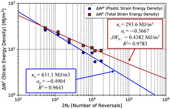
Figure 16.
Total and plastic strain energy densities at the half-life as a function of the number of reversals to failure.
Quantitatively, taking the parameter as a reference, the slope of the model is inferior, which means the elastic energy density associated with the tensile stress per cycle, , has a strong weight in its contribution to , mainly for higher lives. Table 7 summarises the respective coefficients and exponents for models (7) and (8). For the − model, the residual elastic strain energy density, , of 0.4382 was determined for a fatigue limit, = 420.7 MPa. If we consider a value 10% higher than as the threshold of the fatigue limit, an “infinite” life, , of 2.72 × 10¹⁰ reversals is found. For both models, a good fitting was determined with and for − and − representations, respectively.
Comparing with tempered 51CrV4 steel at 540–650C [6], the model predicts the higher fatigue resistance of 51CrV4 steel when tempered at 450C, due to the coefficient and exponent both being higher.
5.7. Micro-Mechanisms and Failure Modes
In materials under low-cycle fatigue conditions, even in high-strength ones with small amounts of plastic strain, the normal direction of the fracture plane might not be the same as that exhibited by specimens under monotonic loading (see Figure 6). Figure 17 shows a representative comparison of failure modes for specimens tested at distinct strain amplitudes. One verifies that most samples exhibited a fracture plane oriented at 45° in relation to the principal stress direction (see Figure 17B,C). However, in one case, the crack propagates perpendicularly to the applied load direction (see Figure 17A). This case corresponds to an applied total strain of , and the fatigue fracture surfaces have the same appearance as semi-brittle materials operating in a high-cycle fatigue regime.
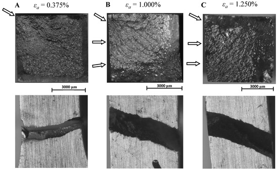
Figure 17.
Visual comparison of specimen failures depending on the applied strain: (A)—Low strain level; (B)—Medium strain level; (C)—High strain level.
The fracture surfaces presented in Figure 17 were submitted to scanning electron microscopy, SEM. The SEM analysis was performed with the FEI Quanta 400 FEG ESEM/EDAX Genesis X4M scanning electron microscope (Hillsboro, OR, USA). The analysis’s description of the failure micro-mechanisms will begin from an overall perspective, followed by the microscopy analysis in the initiation zones, crack propagation, and proximity of the total fracture zone.
Figure 18 depicts the occurrence of multiple crack fronts initiated on different sites of the specimen which led to the formation of different propagation planes. The analysis zone is identified with points with different geometries. For the specimen subjected to a strain amplitude level of 1.00%, the development of ductile-dimples structures with micro-cavities (see Figure 18B,C) was observed both in the initiation (circle) and propagation (triangle) zones. As the crack advances to the diamond point (Figure 18D), one verifies a change from ductile failure mechanisms to cleavage mechanisms (cleavage facets). The crack propagation is essentially transgranular without any apparent existence of local micro-cavities produced by decohesion or fracture of particles of more brittle inclusions [47].
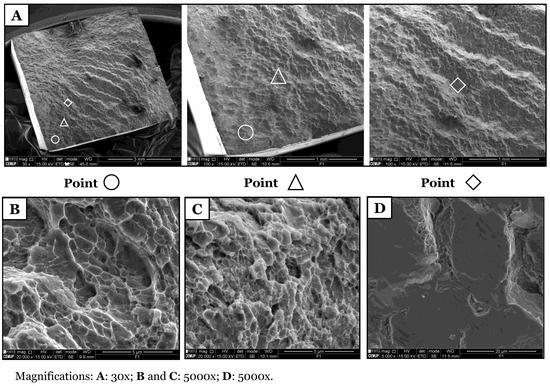
Figure 18.
Visual comparison of specimen failures under a strain amplitude level of 1.00%.
Evaluating the fracture surfaces of samples subjected to different strain amplitude conditions, A— = 1.000%, B— = 1.250%, and C— = 0.375% (Figure 19), the crack propagation mechanism is always transgranular. According to Figure 19, if the applied strain amplitude is increased to 1.250% (Figure 19B), multiple-crack nucleation on the periphery of the specimen occurs. Microscopically, higher deformation levels lead to fracture initiation and propagation zones (circle point) with ductile-dimples, micro-cavities, and the coalescence of voids around heterogeneities.
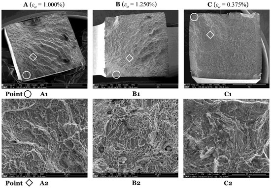
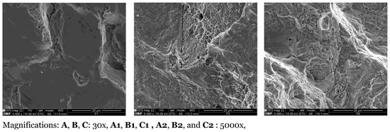
Figure 19.
Visual comparison of specimen failures depending on the applied strain.
However, for lower strain levels close to the threshold of the plastic yield, (Figure 19C), the fracture surface might demonstrate a typically macroscopic semi-brittle fracture surface, whose surface presents micro-cleavage, with cleavage cracks. As the crack advances to an unstable fracture zone (diamond point), mixed failure modes with a high predominance of cleavage mechanisms are identified.
6. Conclusions
The 51CrV4 steel was analysed in terms of monotonic and cyclic fatigue strengths. Monotonic tests allowed for the verification of a high level of resilience, with a yield stress of MPa, but a low ductility, . Regarding the Ramberg–Osgood, RO, relationship, a hardening coefficient, K, of MPa and a hardening exponent, n, of were determined.
From cyclic tests under strain-controlled conditions, the chromium-vanadium alloy steel exhibited a cyclic softening behaviour with cyclic mean stress relaxation when tested at a strain ratio of 0.0. A power law was suggested in this article to describe the cyclic softening of the stress amplitude and the mean stress relaxation, resulting in the coefficients and , and exponents and , respectively.
Regarding cyclic tests, the RO stabilised cyclic curve was well-fitted with the parameters MPa and . These parameters were compared with the ones obtained from estimation models based on monotonic mechanical properties, and no significant differences were found. Using the master curve methodology, a slight deviation of the material in relation to a Masing-type behaviour was observed, with MPa and .
With respect to fatigue life models, strain-life and energy-life ones were considered in the analysis. The CMB model was fitted with the following parameters: = 1693.37 MPa, = −0.1022, = 1.624, and = −0.8015. Compared with the MUSM, MFPM, and MM estimation models, a large difference associated with and was observed. However, considering only the fatigue data whose mean stress level has undergone a strong relaxation, better results are obtained, such that = 1565.36 MPa, = −0.0919, = 0.2320, and = −0.5282 may be considered for a strain ratio of −1. Additionally, energy-based models prove to be suitable for fatigue with a mean stress effect from low-cycle to high-cycle regimes when the total strain energy density model with = , , and the residual strain energy density , of was considered. Compared with the same steel, with the same chemical composition, but heat-treated with a higher tempering temperature, the fatigue resistance was higher, as observed in other investigations already carried out on martensitic steels for different tempering temperatures.
Both fatigue prediction models obtained a good prediction in regard to the experimental data, which indicated that both can be considered in future fatigue prediction analyses of these components, or components produced with the same material. However, since the energy model presents advantages over fatigue prediction models where only the strain component is considered, and combined with the fact that the energy model considers residual strain energy associated with the fatigue limit stress and is less sensitive to the mean component of the load, the energy model may be a better option.
Lastly, SEM analysis at the fracture surfaces revealed a transgranular propagation crack with multi-crack initiation fronts in most of the samples. Except in one sample, most samples exhibited a fracture surface whose plane is not perpendicular to the loading direction. In the exception, a typical fracture in specimens operating in the high-cycle regime was found. Most samples having an oblique fracture developed ductile-dimple structures with micro-cavities and voids around heterogeneities (at the initiation and propagation zones). The ductile failure mechanisms change to cleavage facets at the nearby unstable fracture zone. For cracks propagating perpendicularly to the load, failure micro-mechanisms essentially occur via the cleavage, with the appearance of cleavage cracks in the initiation zone.
Author Contributions
Conceptualization, V.M.G.G. and C.D.S.S.; methodology, V.M.G.G. and C.D.S.S.; software, V.M.G.G. and C.D.S.S.; validation, V.M.G.G., J.A.F.O.C. and A.M.P.d.J.; formal analysis, V.M.G.G. and C.D.S.S.; investigation, V.M.G.G. and C.D.S.S.; resources, J.A.F.O.C. and A.M.P.d.J.; data curation, V.M.G.G. and C.D.S.S.; writing—original draft preparation, V.M.G.G.; writing—review and editing, V.M.G.G., and C.D.S.S., J.A.F.O.C. and A.M.P.d.J.; visualization, V.M.G.G. and C.D.S.S.; supervision, J.A.F.O.C. and A.M.P.d.J.; project administration, A.M.P.d.J.; funding acquisition, J.A.F.O.C. and A.M.P.d.J. All authors have read and agreed to the published version of the manuscript.
Funding
The authors also want to express a special thanks to the Doctoral Programme iRail—Innovation in Railway Systems and Technologies funded by the Portuguese Foundation for Science and Technology, IP (FCT) through the PhD grant (PD/BD/143141/2019); and the following Research Projects: FERROVIA 4.0, with reference POCI-01-0247-FEDER-046111, co-financed by the European Regional Development Fund (ERDF), through the Operational Programme for Competitiveness and Internationalization (COMPETE 2020), under the PORTUGAL 2020 Partnership Agreement; SMARTWAGONS—DEVELOPMENT OF PRODUCTION CAPACITY IN PORTUGAL OF SMART WAGONS FOR FREIGHT with reference nr. C644940527-00000048, investment project nr.27 from the Incentive System to Mobilising Agendas for Business Innovation, funded by the Recovery and Resilience Plan and by European Funds NextGeneration EU; and PRODUCING RAILWAY ROLLING STOCK IN PORTUGAL, with reference nr. C645644454-00000065, investment project nr. 55 from the Incentive System to Mobilising Agendas for Business Innovation, funded by the Recovery and Resilience Plan and by European Funds NextGeneration EU. And a final thank you to CEMUP, “Centro de Materiais da Universidade do Porto”, and respective technical staff for carrying out the scanning electron microscopy tests.
Data Availability Statement
The data presented in this study are available on request from the corresponding author. The data are not publicly available due to privacy restrictions.
Conflicts of Interest
The authors declare no conflicts of interest.
References
- Yamada, Y.; Kuwabara, T. Materials for Springs; Springer: Berlin/Heidelberg, Germany, 2007. [Google Scholar] [CrossRef]
- Smith, W.F. Principles of Materials Science and Engineering, 3rd ed.; Mc Graw-Hill Book Company: New York, NY, USA, 1999. [Google Scholar]
- Li, H.Y.; Hu, J.D.; Li, J.; Chen, G.; Xiong-Jie, S. Effect of tempering temperature on microstructure and mechanical properties of AISI 6150 steel. J. Cent. South Univ. 2013, 20, 866–870. [Google Scholar] [CrossRef]
- Brnic, J.; Brcic, M.; Krscanski, S.; Canadija, M.; Niu, J. Analysis of materials of similar mechanical behavior and similar industrial assignment. Procedia Manuf. 2019, 37, 207–213. [Google Scholar] [CrossRef]
- Han, X.; Zhang, Z.; Hou, J.; Thrush, S.J.; Barber, G.C.; Zou, Q.; Yang, H.; Qiu, F. Tribological behavior of heat treated AISI 6150 steel. J. Mater. Res. Technol. 2020, 9, 12293–12307. [Google Scholar] [CrossRef]
- Gomes, V.M.G.; Eck, S.; De Jesus, A.M.P. Cyclic Hardening and Fatigue Damage Features of 51CrV4 Steel for the Crossing Nose Design. Appl. Sci. 2023, 13, 8308. [Google Scholar] [CrossRef]
- Akiniwa, Y.; Stanzl-Tschegg, S.; Mayer, H.; Wakita, M.; Tanaka, K. Fatigue strength of spring steel under axial and torsional loading in the very high cycle regime. Int. J. Fatigue 2008, 30, 2057–2063. [Google Scholar] [CrossRef]
- Jaramillo, S.H.E.; de Sánchez, N.A.; Avila, D.J.A. Effect of the shot peening process on the fatigue strength of SAE 5160 steel. J. Mech. Eng. Sci. 2019, 233, 4328–4335. [Google Scholar] [CrossRef]
- Gomes, V.M.G.; De Jesus, A.M.; Figueiredo, M.; Correia, J.A.; Calcada, R. Fatigue Failure of 51CrV4 Steel Under Rotating Bending and Tensile. In Fatigue and Fracture of Materials and Structures: Contributions from ICMFM XX and KKMP2021; Springer International Publishing: Cham, Switzerland, 2022; Volume 8, pp. 307–313. [Google Scholar] [CrossRef]
- Sustarsic, B.; Borkovic, P.; Echlseder, W.; Gerstmayr, G.; Javidi, A.; Sencic, B. Fatigue strength and microstructural features of spring steel. Struct. Integr. Life 2011, 11, 27–34. [Google Scholar]
- Soady, K.A. Life assessment methodologies incorporating shot peening process effects: Mechanistic consideration of residual stresses and strain hardening: Part 1—Effect of shot peening on fatigue resistance. Mater. Sci. Technol. 2013, 29, 637–651. [Google Scholar] [CrossRef]
- Llaneza, V.; Belzunce, F. Study of the effects produced by shot peening on the surface of quenched and tempered steels: Roughness, residual stresses and work hardening. Appl. Surf. Sci. 2015, 356, 475–485. [Google Scholar] [CrossRef]
- Petrovi, D.; Bii Gai, M.; Savkovi, M. Increasing the efficiency of railway transport by improvement of suspension of freight wagons. Promet-Traffic Transp. 2012, 24, 487–493. [Google Scholar] [CrossRef]
- Ceyhanli, U.T.; Bozca, M. Experimental and numerical analysis of the static strength and fatigue life reliability of parabolic leaf springs in heavy commercial trucks. Adv. Mech. Eng. 2020, 12. [Google Scholar] [CrossRef]
- Infante, V.; Freitas, M.; Baptista, R. Failure analysis of a parabolic spring belonging to a railway wagon. Int. J. Fatigue 2022, 140, 106526. [Google Scholar] [CrossRef]
- Gomes, V.; Correia, J.; Calçada, R.; Barbosa, R.; de Jesus, A. Fatigue in trapezoidal leaf springs of suspensions in two-axle wagons—An overview and simulation. In Structural Integrity and Fatigue Failure Analysis; Lesiuk, G., Szata, M., Blazejewski, W., de Jesus, A.M., Correia, J.A., Eds.; VCMF 2020 Structural Integrity; Springer: Berlin/Heidelberg, Germany, 2022; Volume 25, pp. 97–114. [Google Scholar] [CrossRef]
- Clarke, C.; Borowski, G. Evaluation of a leaf spring failure. J. Fail. Anal. Prev. 2005, 5, 54–63. [Google Scholar] [CrossRef]
- Bergh, F.; Silva, G.C.; Silva, C.; Paiva, P. Analysis of an automotive coil spring fracture. Eng. Fail. Anal. 2021, 129, 105679. [Google Scholar] [CrossRef]
- Fragoudakis, R.; Saigal, A.; Savaidis, G.; Malikoutsakis, M.; Bazios, I.; Savaidis, A.; Pappas, G.; Karditsas, S. Fatigue assessment and failure analysis of shot-peened leaf springs. Fatigue Fract. Eng. Mater. Struct. 2013, 36, 92–101. [Google Scholar] [CrossRef]
- Ince, A.; Glinka, G. A numerical method for elasto-plastic notch-root stress–strain analysis. J. Strain Anal. Eng. Des. 2013, 48, 229–244. [Google Scholar] [CrossRef]
- Dabiri, M.; Isakov, M.; Skriko, T.; Björk, A. Experimental fatigue characterization and elasto-plastic finite element analysis of notched specimens made of direct-quenched ultra-high-strength steel. Proc. Inst. Mech. Eng. Part C J. Mech. Eng. Sci. 2017, 231, 4209–4226. [Google Scholar] [CrossRef]
- Kiani, M.; Ishak, J.; Keller, M.W.; Tipton, S. Comparison between nonlinear FEA and notch strain analysis for modeling elastoplastic stress-strain response in crossbores. Int. J. Mech. Sci. 2016, 118, 45–54. [Google Scholar] [CrossRef]
- Raposo, P.; Correia, J.A.F.O.; De Jesus, A.M.P.; Calçada, R.; Lesiuk, G.; Hebdon, M.; Fernández Canteli, A.C. Probabilistic fatigue SN curves derivation for notched components. Frat. Integrita Strutt. 2017, 11. [Google Scholar] [CrossRef]
- Pereira, H.F.; De Jesus, A.M.; Ribeiro, A.S.; Fernandes, A.A. Fatigue modeling of a notched flat plate under variable amplitude loading supported by elastoplastic finite element method analyses. J. Pressure Vessel Technol. 2011, 133, 061207. [Google Scholar] [CrossRef]
- Yang, G.; Xia, S.L.; Zhang, F.C.; Branco, R.; Long, X.Y.; Li, Y.G.; Li, J.H. Effect of tempering temperature on monotonic and low-cycle fatigue properties of a new low-carbon martensitic steel. Mater. Sci. Eng. A 2021, 826, 141939. [Google Scholar] [CrossRef]
- Kanazawa, K.; Kimura, M.; Abe, T.; Ueda, I.; Muramatsu, K. Low-Cycle Fatigue Behavior of Spring Steels. Trans. Jpn. Soc. Spring Eng. 1995, 40, 5–14. [Google Scholar] [CrossRef][Green Version]
- Li, D.; Kim, K.; Lee, C. Low cycle fatigue data evaluation for a high-strength spring steel. Int. J. Fatigue 1997, 19, 607–612. [Google Scholar] [CrossRef]
- Kwon, H.; Barlat, F.; Lee, M.; Chung, Y.; Uhm, S. Influence of tempering temperature on low cycle fatigue of high strength steel. ISIJ Int. 2014, 54, 979–984. [Google Scholar] [CrossRef]
- Sorokin, G.M.; Bobrov, S.N. Effect of tempering temperature on the fatigue strength of high-strength tool steel. Met. Sci. Heat Treat. 1974, 16, 755–757. [Google Scholar] [CrossRef]
- Gomes, V.M.; de Jesus, A.M.; Correia, J.; Calçada, R. Determination of the Highest Potential Spots for Fatigue Failure in Parabolic Leaf Springs using the Maximum Variance Approach. Procedia Struct. Integr. 2022, 42, 1552–1559. [Google Scholar] [CrossRef]
- Matej, J.; Seńko, J.; Awrejcewicz, J. Dynamic properties of two-axle freight wagon with uic double-link suspension as a non-smooth system with dry friction. In Applied Non-Linear Dynamical Systems. Springer Int. Publ. 2014, 19, 255–268. [Google Scholar] [CrossRef]
- Ince, A.; Glinka, G. A modification of Morrow and Smith–Watson–Topper mean stress correction models. Fatigue Fract. Eng. Mater. Struct. 2011, 34, 854–867. [Google Scholar] [CrossRef]
- Schäfer, B.J.; Sonnweber-Ribic, P.; Ul Hassan, H.; Hartmaier, A. Micromechanical modelling of the influence of strain ratio on fatigue crack initiation in a martensitic steel-a comparison of different fatigue indicator parameters. Materials 2019, 12, 2852. [Google Scholar] [CrossRef] [PubMed]
- Gong, X.; Wang, T.; Li, Q.; Liu, Y.; Zhang, H.; Zhang, W.; Wang, Q. Cyclic responses and microstructure sensitivity of Cr-based turbine steel under different strain ratios in low cycle fatigue regime. Mater. Des. 2021, 201, 109529. [Google Scholar] [CrossRef]
- Branco, R.; Costa, J.D.; Borrego, L.P.; Wu, S.C.; Long, X.Y.; Zhang, F.C. Effect of strain ratio on cyclic deformation behaviour of 7050-T6 aluminum alloy. Int. J. Fatigue 2019, 129, 105234. [Google Scholar] [CrossRef]
- Zhang, J.; Li, W.; Dai, H.; Liu, N.; Lin, J. Study on the elastic–plastic correlation of low-cycle fatigue for variable asymmetric loadings. Materials 2019, 13, 2451. [Google Scholar] [CrossRef] [PubMed]
- Miner, M.A. Cumulative damage in fatigue. J. Appl. Mech. 1945, 12, A159–A164. [Google Scholar] [CrossRef]
- Liu, R.; Zhang, Z.J.; Zhang, P.; Zhang, Z.F. Extremely-low-cycle fatigue behaviours of Cu and Cu–Al alloys: Damage mechanisms and life prediction. Acta Mater. Des. 2015, 83, 341–356. [Google Scholar] [CrossRef]
- Ramberg, W.; Osgood, W.R. Description of stress-strain curves by three parameters. Natl. Advis. Comm. Aeronaut. 1943. Available online: https://ntrs.nasa.gov/api/citations/19930081614/downloads/19930081614.pdf (accessed on 19 February 2024).
- Nejad, R.M.; Berto, F. Fatigue fracture and fatigue life assessment of railway wheel using non-linear model for fatigue crack growth. Int. J. Fatigue 2021, 153, 106516. [Google Scholar] [CrossRef]
- Correia, J.A.F.O.; da Silva, A.L.; Xin, H.; Lesiuk, G.; Zhu, S.P.; de Jesus, A.M.P.; Fernandes, A.A. Fatigue performance prediction of S235 base steel plates in the riveted connections. Structures 2021, 30, 745–755. [Google Scholar] [CrossRef]
- Qiang, B.; Liu, X.; Liu, Y.; Yao, C.; Li, Y. Experimental study and parameter determination of cyclic constitutive model for bridge steels. J. Constr. Steel Res. 2021, 183, 106738. [Google Scholar] [CrossRef]
- Kreithner, M.; Niederwanger, A.; Lang, R. Influence of the Ductility Exponent on the Fatigue of Structural Steels. Metals 2023, 13, 759. [Google Scholar] [CrossRef]
- Nejad, R.M.; Berto, F. Fatigue crack growth of a railway wheel steel and fatigue life prediction under spectrum loading conditions. Int. J. Fatigue 2022, 153, 106516. [Google Scholar] [CrossRef]
- Hu, Y.; Shi, J.; Cao, X.; Zhi, J. Low cycle fatigue life assessment based on the accumulated plastic strain energy density. Materials 2021, 14, 2372. [Google Scholar] [CrossRef] [PubMed]
- Souto, C.D.; Gomes, V.M.G.; Da Silva, L.F.; Figueiredo, M.V.; Correia, J.A.F.O.; Lesiuk, G.; Fernandes, A.A.; De Jesus, A.M.P. Global-local fatigue approaches for snug-tight and preloaded hot-dip galvanized steel bolted joints. Int. J. Fatigue 2021, 153, 106486. [Google Scholar] [CrossRef]
- Branco, R.; Costa, J.D.; Antunes, F.V. Low-cycle fatigue behaviour of 34CrNiMo6 high strength steel. Theor. Appl. Fract. Mech. 2012, 58, 28–34. [Google Scholar] [CrossRef]
- Lefebvre, D.; Ellyin, F. Cyclic response and inelastic strain energy in low cycle fatigue. Int. J. Fatigue 1948, 6, 9–15. [Google Scholar] [CrossRef]
- Kujawski, D.; Ellyin, F. A cumulative damage theory for fatigue crack initiation and propagation. Int. J. Fatigue 1948, 6, 83–88. [Google Scholar] [CrossRef]
- Jhansale, H.R.; Topper, T.H. Engineering Analysis of the Inelastic Stress Response of a Structural Metal Under Variable Cyclic Strains; ASTM International: West Conshohocken, PA, USA, 1971; pp. 246–270. [Google Scholar] [CrossRef]
- Ellyin, F.; Kujawski, D. Plastic Strain Energy in Fatigue Failure. J. Pressure Vessel Technol. 1948, 106, 342–347. [Google Scholar] [CrossRef]
- Ellyin, F. Fatigue Damage, Crack Growth and Life Prediction; Springer: Berlin/Heidelberg, Germany, 2012. [Google Scholar] [CrossRef]
- Coffin, J.L.F., Jr. A study of the effects of cyclic thermal stresses on a ductile metal. Trans. Am. Soc. Mech. Eng. 1954, 76, 931–949. [Google Scholar] [CrossRef]
- Manson, S.S. Behavior of materials under conditions of thermal stress. In National Advisory Committee for Aeronautics; NASA: Washington, DC, USA, 1954. [Google Scholar]
- Morrow, J.D. Cyclic plastic strain energy and fatigue of metals. Int. Frict. Damping And Cyclic Plast. 1969, 378, 45–87. [Google Scholar] [CrossRef]
- Ellyin, F. Fatigue Damage, Crack Growth and Life Prediction, 1st ed.; Chapman and Hall: London, UK, 1997. [Google Scholar]
- Branco, R.; Costa, J.D.; Antunes, F.V.; Perdigão, S. Monotonic and cyclic behavior of DIN 34CrNiMo6 tempered alloy steel. Metals 2016, 6, 98. [Google Scholar] [CrossRef]
- Golos, K.; Ellyin, F. Generalization of cumulative damage criterion to multilevel cyclic loading. Theor. Appl. Fract. Mech. 1987, 7, 169–176. [Google Scholar] [CrossRef]
- Mahtabi, M.J.; Shamsaei, N. A modified energy-based approach for fatigue life prediction of superelastic NiTi in presence of tensile mean strain and stress. Int. J. Mech. Sci. 2016, 117, 321–333. [Google Scholar] [CrossRef]
- NP EN 10002-1; Metallic Materials—Tensile Testing—Part 1: Method of Test at Ambient Temperature. European Committee for Standardization (CEN): Brussels, Belgium, 2001.
- ISO 6892-1; Metallic Materials-Tensile Testing-Part 1: Method of Test at Ambient Temperature. European Committee for Standardization: Brussels, Belgium, 2009.
- ASTM E111-04; Standard Test Method for Young’s Modulus, Tangent Modulus, and Chord Modulus, (Reapproved 2010). ASTM International: West Conshohocken, PA, USA, 2010. [CrossRef]
- ASTM E606; Standard Test Method for Strain-Controlled Fatigue Testing. Annual Book of ASTM Standards: Leeds, UK, 1998; pp. 1–15.
- Montgomery, D.C.; Runger, G.C. Applied Statistics and Probability for Engineers, 6th ed.; Wiley: Hoboken, NJ, USA, 2013. [Google Scholar]
- ASTM E739-23; Standard Guide for Statistical Analysis of Linear or Linearized Stress-Life (S-N) and Strain-Life (ε-N) Fatigue Data. American Society for Testing and Materials: West Conshohocken, PA, USA, 2023.
- Drozdov, A.V. Longitudinal elastic modulus and Poisson’s ratio computations with automatic experimental data processing of the materials. Strength Mater. 2020, 52, 329–337. [Google Scholar] [CrossRef]
- Chen, R.; Wang, Z.; Zhu, F.; Zhao, H.; Qin, J.; Zhong, L. Effects of rare-earth micro-alloying on microstructures, carbides, and internal friction of 51CrV4 steels. J. Alloys Compds. 2020, 824, 153849. [Google Scholar] [CrossRef]
- Mohanty, S.; Soppet, W.K.; Barua, B.; Majumdar, S.; Natesan, K. Modeling the cycle-dependent material hardening behavior of 508 low alloy steel. Exp. Mech. 2017, 57, 847–855. [Google Scholar] [CrossRef]
- Lopez, Z.; Fatemi, A. A method of predicting cyclic stress–strain curve from tensile properties for steels. Mater. Sci. Eng. A 2012, 556, 540–550. [Google Scholar] [CrossRef]
- Song, W.; Liu, X.; Berto, F.; Razavi, N. Low-cycle fatigue behavior of 10CrNi3MoV high strength steel and its undermatched welds. Materials 2018, 11, 661. [Google Scholar] [CrossRef] [PubMed]
- Muralidharan, U.; Manson, S.S. A modified universal slopes equation for estimation of fatigue characteristics of metals. J. Eng. Mater. Technol. 1988, 110, 55–58. [Google Scholar] [CrossRef]
- Yang, S.; Yang, L.; Wang, Y. Determining the fatigue parameters in total strain life equation of a material based on monotonic tensile mechanical properties. Eng. Fract. Mech. 1987, 226, 106866. [Google Scholar] [CrossRef]
- Meggiolaro, M.A.; Castro, J.T.P. Statistical evaluation of strain-life fatigue crack initiation predictions. Int. J. Fatigue 2004, 26, 463–476. [Google Scholar] [CrossRef]
- Ince, A.; Glinka, G. A generalized fatigue damage parameter for multiaxial fatigue life prediction under proportional and non-proportional loadings. Int. J. Fatigue 2014, 62, 34–41. [Google Scholar] [CrossRef]
- Milovanović, V.; Arsić, D.; Milutinović, M.; Živković, M.; Topalović, M. Comparison Study of Fatigue Behavior of S355J2+ N, S690QL and X37CrMoV5-1 Steel. Metals 2022, 12, 1199. [Google Scholar] [CrossRef]


Disclaimer/Publisher’s Note: The statements, opinions and data contained in all publications are solely those of the individual author(s) and contributor(s) and not of MDPI and/or the editor(s). MDPI and/or the editor(s) disclaim responsibility for any injury to people or property resulting from any ideas, methods, instructions or products referred to in the content. |
© 2024 by the authors. Licensee MDPI, Basel, Switzerland. This article is an open access article distributed under the terms and conditions of the Creative Commons Attribution (CC BY) license (https://creativecommons.org/licenses/by/4.0/).