Identification of Sheet Metal Constitutive Parameters Using Metamodeling of the Biaxial Tensile Test on a Cruciform Specimen

 , ,
, ,  ,
,  and
and
Abstract
1. Introduction
2. Numerical Model

3. Identification Strategy
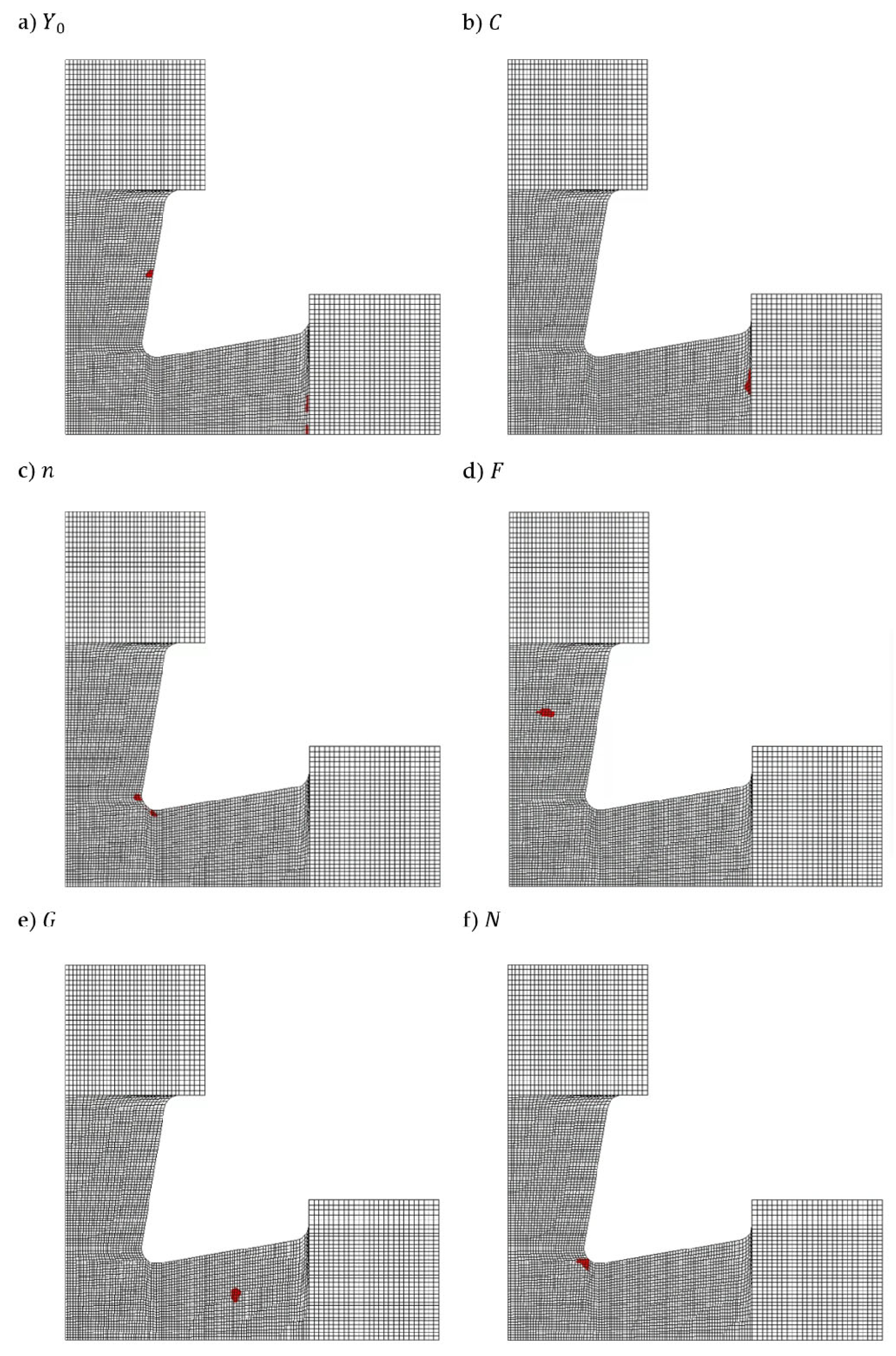
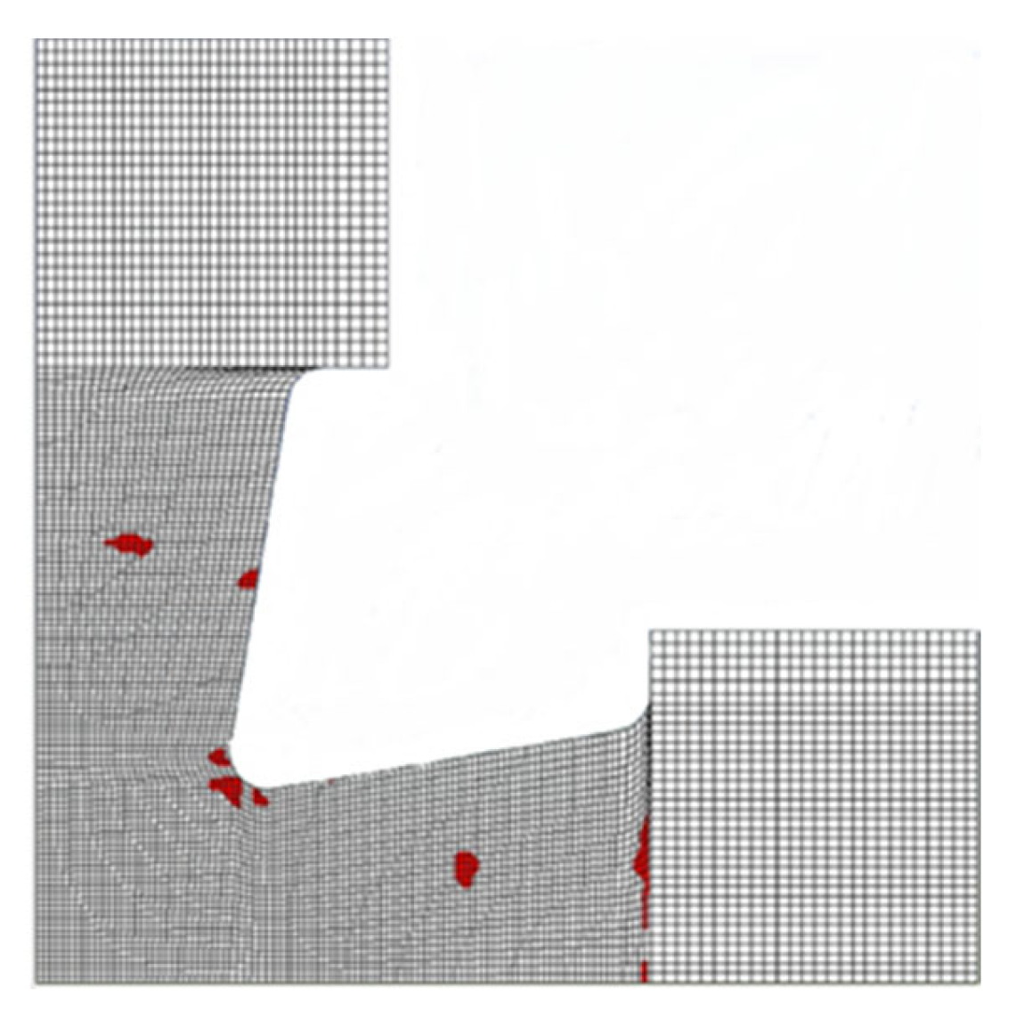
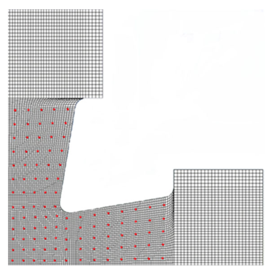
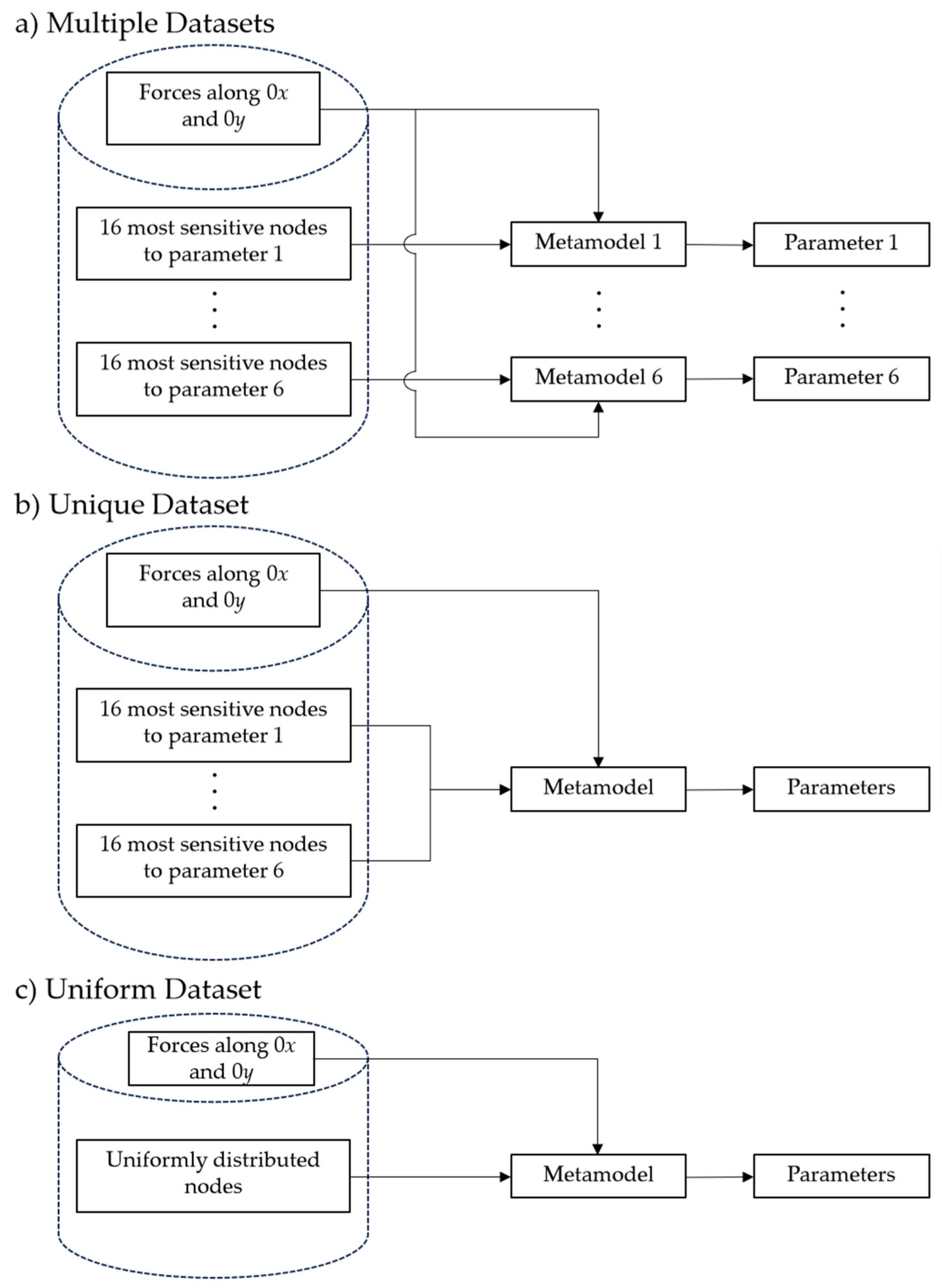
3.1. Strategy Design
3.2. Machine Learning Technique
3.3. Dataset Generation
3.4. Performance Metric
4. Strategy Results
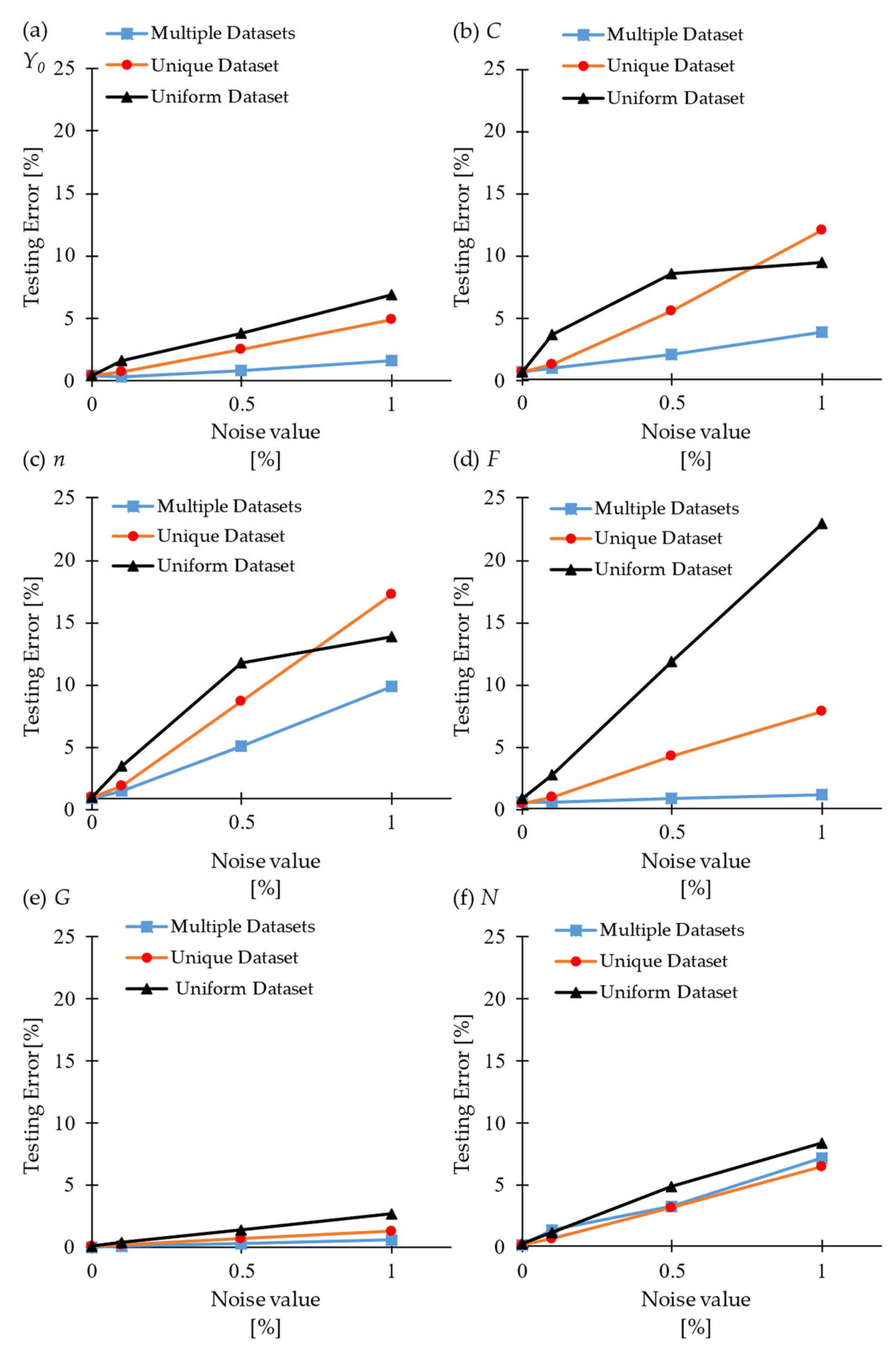
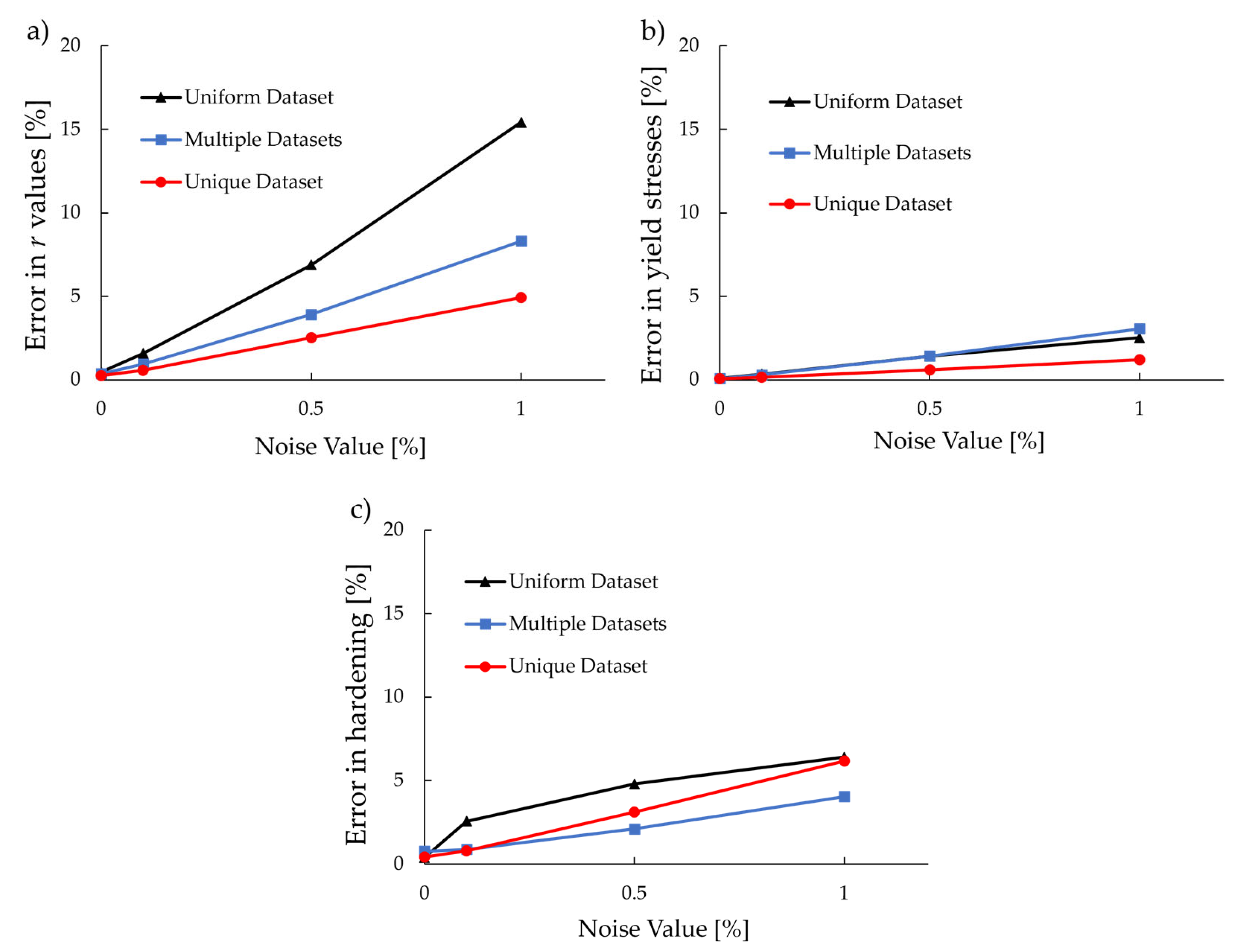
5. Noise Analysis
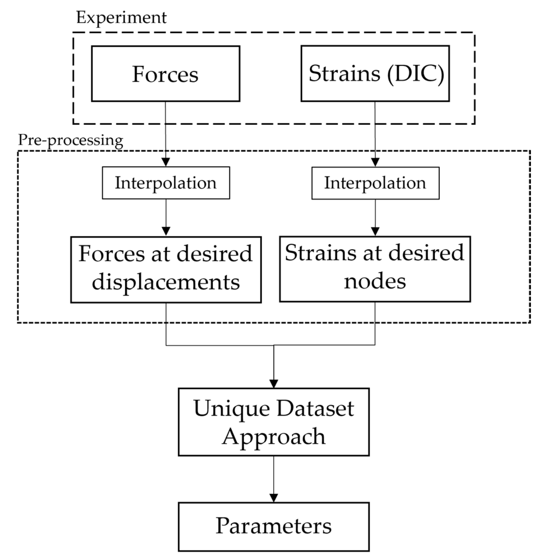
Envisaged Experimental Setup
6. Conclusions
Author Contributions
Funding
Data Availability Statement
Conflicts of Interest
Abbreviations
| DD3IMP | Deep Drawing 3D IMPlicit; |
| DIC | Digital Image Correlation; |
| FEA | Finite Element Analysis; |
| FEMU | Finite Element Model Updating; |
| GPR | Gaussian Process Regression; |
| LBFGS | Limited-Memory Broyden–Fletcher–Goldfarb–Shanno; |
| RBF | Radial Basis Function; |
| SCG | Scaled Conjugate Gradient; |
| TNC | Truncated Newton. |
References
- Hu, W.; Yao, L.G.; Hua, Z.Z. Optimization of Sheet Metal Forming Processes by Adaptive Response Surface Based on Intelligent Sampling Method. J. Mater. Process Technol. 2008, 197, 77–88. [Google Scholar] [CrossRef]
- Chou, I.-N.; Hung, C. Finite Element Analysis and Optimization on Springback Reduction. Int. J. Mach. Tools Manuf. 1999, 39, 517–536. [Google Scholar] [CrossRef]
- Trzepieciński, T.; Gelgele, H.L. Investigation of Anisotropy Problems in Sheet Metal Forming Using Finite Element Method. Int. J. Mater. Form. 2011, 4, 357–369. [Google Scholar] [CrossRef]
- Hill, R. A Theory of the Yielding and Plastic Flow of Anisotropic Metals. Proc. R. Soc. Lond. Ser. A Math. Phys. Sci. 1948, 67, 281–297. [Google Scholar]
- Meyer, L.W.; Abdel-Malek, S.; Herzig, N. Experimental Methods for Characterizing of Sheet Metals at High Strain Rates. Key Eng. Mater. 2011, 473, 474–481. [Google Scholar] [CrossRef]
- Brosius, A.; Yin, Q.; Güner, A.; Tekkaya, A.E. A New Shear Test for Sheet Metal Characterization. Steel Res. Int. 2011, 82, 323–328. [Google Scholar] [CrossRef]
- Yin, Q.; Zillmann, B.; Suttner, S.; Gerstein, G.; Biasutti, M.; Tekkaya, A.E.; Wagner, M.F.X.; Merklein, M.; Schaper, M.; Halle, T.; et al. An Experimental and Numerical Investigation of Different Shear Test Configurations for Sheet Metal Characterization. Int. J. Solids Struct. 2014, 51, 1066–1074. [Google Scholar] [CrossRef]
- Pereira, A.F.G.; Prates, P.A.; Oliveira, M.C.; Fernandes, J.V. Inverse Identification of the Work Hardening Law from Circular and Elliptical Bulge Tests. J. Mater. Process Technol. 2020, 279, 116573. [Google Scholar] [CrossRef]
- Vucetic, M.; Bouguecha, A.; Peshekhodov, I.; Götzea, T.; Huinink, T.; Friebe, H.; Möller, T.; Behrens, B.A. Numerical Validation of Analytical Biaxial True Stress—True Strain Curves from the Bulge Test. AIP Conf. Proc. 2011, 1383, 107–114. [Google Scholar]
- Yoshida, K. Evaluation of Stress and Strain Measurement Accuracy in Hydraulic Bulge Test with the Aid of Finite-Element Analysis. ISIJ Int. 2013, 53, 86–95. [Google Scholar] [CrossRef]
- Habraken, A.M.; Aksen, T.A.; Alves, J.L.; Amaral, R.L.; Betaieb, E.; Chandola, N.; Corallo, L.; Cruz, D.J.; Duchêne, L.; Engel, B.; et al. Analysis of ESAFORM 2021 Cup Drawing Benchmark of an Al Alloy, Critical Factors for Accuracy and Efficiency of FE Simulations. Int. J. Mater. Form. 2022, 15, 61. [Google Scholar] [CrossRef]
- Prates, P.A.; Pereira, A.F.G.; Sakharova, N.A.; Oliveira, M.C.; Fernandes, J. V Inverse Strategies for Identifying the Parameters of Constitutive Laws of Metal Sheets. Adv. Mater. Sci. Eng. 2016, 2016, 4152963. [Google Scholar] [CrossRef]
- Zhang, Y.; Gothivarekar, S.; Conde, M.; Van de Velde, A.; Paermentier, B.; Andrade-Campos, A.; Coppieters, S. Enhancing the Information-Richness of Sheet Metal Specimens for Inverse Identification of Plastic Anisotropy through Strain Fields. Int. J. Mech. Sci. 2022, 214, 106891. [Google Scholar] [CrossRef]
- Souto, N.; Andrade-Campos, A.; Thuillier, S. Mechanical Design of a Heterogeneous Test for Material Parameters Identification. Int. J. Mater. Form. 2017, 10, 353–367. [Google Scholar] [CrossRef]
- Conde, M.; Henriques, J.; Coppieters, S.; Andrade-Campos, A. Parameter Identification of Swift Law Using a FEMU-Based Approach and an Innovative Heterogeneous Mechanical Test. Key Eng. Mater. 2022, 926, 2238–2246. [Google Scholar] [CrossRef]
- Makinde, A.; Thibodeau, L.; Neale, K.W. Development of an Apparatus for Biaxial Testing Using Cruciform Specimens. Exp. Mech. 1992, 32, 138–144. [Google Scholar] [CrossRef]
- Cooreman, S.; Lecompte, D.; Sol, H.; Vantomme, J.; Debruyne, D. Identification of Mechanical Material Behavior through Inverse Modeling and DIC. Exp. Mech. 2008, 48, 421–433. [Google Scholar] [CrossRef]
- Zhang, S.; Léotoing, L.; Guines, D.; Thuillier, S. Potential of the Cross Biaxial Test for Anisotropy Characterization Based on Heterogeneous Strain Field. Exp. Mech. 2015, 55, 817–835. [Google Scholar] [CrossRef]
- Prates, P.A.; Oliveira, M.C.; Fernandes, J.V. A New Strategy for the Simultaneous Identification of Constitutive Laws Parameters of Metal Sheets Using a Single Test. Comput. Mater. Sci. 2014, 85, 102–120. [Google Scholar] [CrossRef]
- Siddiqui, A.H.; Patil, J.P.; Mishra, S. Design of a Biaxial Cruciform Specimen with a High Degree of Plastic Deformation and Yield Locus Evolution. Exp. Mech. 2023, 63, 853–869. [Google Scholar] [CrossRef]
- Zhang, R.; Shao, Z.; Shi, Z.; Dean, T.A.; Lin, J. Effect of Cruciform Specimen Design on Strain Paths and Fracture Location in Equi-Biaxial Tension. J. Mater. Process Technol. 2021, 289, 116932. [Google Scholar] [CrossRef]
- Yang, X.; Wu, Z.R.; Yang, Y.R.; Pan, Y.; Wang, S.Q.; Lei, H. Optimization Design of Cruciform Specimens for Biaxial Testing Based on Genetic Algorithm. J. Mater. Eng. Perform. 2023, 32, 2330–2343. [Google Scholar] [CrossRef]
- Chen, J.; Zhang, J.; Zhao, H. Designing a Cruciform Specimen via Topology and Shape Optimisations under Equal Biaxial Tension Using Elastic Simulations. Materials 2022, 15, 5001. [Google Scholar] [CrossRef]
- Deng, N.; Kuwabara, T.; Korkolis, Y.P. Cruciform Specimen Design and Verification for Constitutive Identification of Anisotropic Sheets. Exp. Mech. 2015, 55, 1005–1022. [Google Scholar] [CrossRef]
- Teaca, M.; Charpentier, I.; Martiny, M.; Ferron, G. Identification of Sheet Metal Plastic Anisotropy Using Heterogeneous Biaxial Tensile Tests. Int. J. Mech. Sci. 2010, 52, 572–580. [Google Scholar] [CrossRef]
- Oliveira, M.G.; Martins, J.M.P.; Coelho, B.; Thuillier, S.; Andrade-Campos, A. On the Optimisation Efficiency for the Inverse Identification of Constitutive Model Parameters. In Proceedings of the ESAFORM 2021-24th International Conference on Material Forming, Liege, Belgium, 14–16 April 2021. [Google Scholar]
- Friedlein, J.; Wituschek, S.; Lechner, M.; Mergheim, J.; Steinmann, P. Inverse Parameter Identification of an Anisotropic Plasticity Model for Sheet Metal. IOP Conf. Ser. Mater. Sci. Eng. 2021, 1157, 012004. [Google Scholar] [CrossRef]
- Prates, P.A.; Pereira, A.F.G.; Oliveira, M.C.; Fernandes, J.V. Analytical Sensitivity Matrix for the Inverse Identification of Hardening Parameters of Metal Sheets. Eur. J. Mech. A Solids 2019, 75, 205–215. [Google Scholar] [CrossRef]
- Barton, R.R.; Meckesheimer, M. Chapter 18 Metamodel-Based Simulation Optimization. Handb. Oper. Res. Manag. Sci. 2006, 13, 535–574. [Google Scholar]
- Prates, P.A.; Pinto, J.; Henriques, J. Coupling Machine Learning and Synthetic Image DIC-Based Techniques for the Calibration of Elastoplastic Constitutive Models. Mater. Res. Proc. 2023, 28, 1193–1202. [Google Scholar]
- Jin, R.; Chen, W.; Simpson, T.W. Comparative Studies of Metamodelling Techniques under Multiple Modelling Criteria. Struct. Multidiscip. Optim. 2001, 23, 1–13. [Google Scholar] [CrossRef]
- Huang, C.; El Hami, A.; Radi, B. Metamodel-Based Inverse Method for Parameter Identification: Elastic–Plastic Damage Model. Engineering Optimization. Eng. Optim. 2017, 49, 633–653. [Google Scholar] [CrossRef]
- Cruz, D.J.; Barbosa, M.R.; Santos, A.D.; Miranda, S.S.; Amaral, R.L. Application of Machine Learning to Bending Processes and Material Identification. Metals 2021, 11, 1418. [Google Scholar] [CrossRef]
- Aguir, H.; BelHadjSalah, H.; Hambli, R. Parameter Identification of an Elasto-Plastic Behaviour Using Artificial Neural Networks-Genetic Algorithm Method. Mater. Des. 2011, 32, 48–53. [Google Scholar] [CrossRef]
- Cruz, D.J.; Barbosa, M.R.; Santos, A.D.; Amaral, R.L.; de Sa, J.C.; Fernandes, J.V. Recurrent Neural Networks and Three-Point Bending Test on the Identification of Material Hardening Parameters. Metals 2024, 14, 84. [Google Scholar] [CrossRef]
- Merayo, D.; Rodríguez-Prieto, A.; Camacho, A.M. Topological Optimization of Artificial Neural Networks to Estimate Mechanical Properties in Metal Forming Using Machine Learning. Metals 2021, 11, 1289. [Google Scholar] [CrossRef]
- Xia, J.; Won, C.; Kim, H.; Lee, W.; Yoon, J. Artificial Neural Networks for Predicting Plastic Anisotropy of Sheet Metals Based on Indentation Test. Materials 2022, 15, 1714. [Google Scholar] [CrossRef]
- Liu, S.; Xia, Y.; Shi, Z.; Yu, H.; Li, Z.; Lin, J. Deep Learning in Sheet Metal Bending with a Novel Theory-Guided Deep Neural Network. IEEE CAA J. Autom. Sin. 2021, 8, 565–581. [Google Scholar] [CrossRef]
- Schulz, E.; Speekenbrink, M.; Krause, A. A Tutorial on Gaussian Process Regression: Modelling, Exploring, and Exploiting Functions. J. Math. Psychol. 2018, 85, 1–16. [Google Scholar] [CrossRef]
- Makris, A.; Vandenbergh, T.; Ramault, C.; Van Hemelrijck, D.; Lamkanfi, E.; Van Paepegem, W. Shape Optimisation of a Biaxially Loaded Cruciform Specimen. Polym. Test. 2010, 29, 216–223. [Google Scholar] [CrossRef]
- Oliveira, M.C.; Alves, J.L.; Menezes, L.F. Algorithms and Strategies for Treatment of Large Deformation Frictional Contact in the Numerical Simulation of Deep Drawing Process. Arch. Comput. Methods Eng. 2008, 15, 113–162. [Google Scholar] [CrossRef]
- Neto, D.M.; Oliveira, M.C.; Menezes, L.F. Surface Smoothing Procedures in Computational Contact Mechanics. Arch. Comput. Methods Eng. 2017, 24, 37–87. [Google Scholar] [CrossRef]
- Menezes, L.F.; Teodosiu, C. Three-Dimensional Numerical Simulation of the Deep-Drawing Process Using Solid Finite Elements. J. Mater. Process Technol. 2000, 97, 100–106. [Google Scholar] [CrossRef]
- Pereira, A.F.G.; Oliveira, M.C.; Fernandes, J.V.; Prates, P.A. Variance-Based Sensitivity Analysis of the Biaxial Test on a Cruciform Specimen. Key Eng. Mater. 2022, 926, 2154–2161. [Google Scholar] [CrossRef]
- Swift, H.W. Plastic Instability under Plane Stress. J. Mech. Phys. Solids 1952, 1, 1–18. [Google Scholar] [CrossRef]
- Dong, L.J.; Li, H.; Bo, Z.H. Forming Defects Prediction for Sheet Metal Forming Using Gaussian Process Regression. In Proceedings of the 2017 29th Chinese Control and Decision Conference (CCDC), Chongqing, China, 28–30 May 2017; pp. 472–476. [Google Scholar]
- Gogolashvili, D.; Kozyrskiy, B.; Filippone, M. Locally Smoothed Gaussian Process Regression. In Proceedings of the Procedia Computer Science; Elsevier B.V.: Amsterdam, The Netherlands, 2022; Volume 207, pp. 2717–2726. [Google Scholar]
- The GPy Authors A Gaussian Process Framework in Python. Available online: www.github.com/SheffieldML/GPy (accessed on 3 September 2023).
- Sobol’, I.M. On the Distribution of Points in a Cube and the Approximate Evaluation of Integrals. USSR Comput. Math. Math. Phys. 1967, 7, 86–112. [Google Scholar] [CrossRef]

| Limits | (0.06–1.20) | (0.25–0.625) | (0.4–4.5) | (0.002–0.03) | (0.12–0.25) | (150–1200) |
| Limits | (0.6–3) | (0.6–4.2) | (0.6–5.5) | (150–1200) | (98–1949) | (121–1757) |
Disclaimer/Publisher’s Note: The statements, opinions and data contained in all publications are solely those of the individual author(s) and contributor(s) and not of MDPI and/or the editor(s). MDPI and/or the editor(s) disclaim responsibility for any injury to people or property resulting from any ideas, methods, instructions or products referred to in the content. |
© 2024 by the authors. Licensee MDPI, Basel, Switzerland. This article is an open access article distributed under the terms and conditions of the Creative Commons Attribution (CC BY) license (https://creativecommons.org/licenses/by/4.0/).
Share and Cite
Parreira, T.G.; Marques, A.E.; Sakharova, N.A.; Prates, P.A.; Pereira, A.F.G. Identification of Sheet Metal Constitutive Parameters Using Metamodeling of the Biaxial Tensile Test on a Cruciform Specimen. Metals 2024, 14, 212. https://doi.org/10.3390/met14020212
Parreira TG, Marques AE, Sakharova NA, Prates PA, Pereira AFG. Identification of Sheet Metal Constitutive Parameters Using Metamodeling of the Biaxial Tensile Test on a Cruciform Specimen. Metals. 2024; 14(2):212. https://doi.org/10.3390/met14020212
Chicago/Turabian StyleParreira, Tomás G., Armando E. Marques, Nataliya A. Sakharova, Pedro A. Prates, and André F. G. Pereira. 2024. "Identification of Sheet Metal Constitutive Parameters Using Metamodeling of the Biaxial Tensile Test on a Cruciform Specimen" Metals 14, no. 2: 212. https://doi.org/10.3390/met14020212
APA StyleParreira, T. G., Marques, A. E., Sakharova, N. A., Prates, P. A., & Pereira, A. F. G. (2024). Identification of Sheet Metal Constitutive Parameters Using Metamodeling of the Biaxial Tensile Test on a Cruciform Specimen. Metals, 14(2), 212. https://doi.org/10.3390/met14020212