The Corrosion Behavior of Carbon Steel Materials Used at Nuclear Power Plants During Deactivation and Decommissioning Processes

Abstract

This study is focused on the corrosion behavior of carbon steel A106 B in a static water environment, which simulated the decommissioning transition phase of BWR power plants. When the autoclave was filled with stagnant water, the corrosion rates of carbon steel pipe for the cold-drawn and hot-rolled samples were 23 μm/year and 19 μm/year, respectively. When the autoclave was not completely filled with water, leaving the samples fully submerged, the corrosion rate for the hot-rolled sample increased to 88 μm/year. In an autoclave with periodic water flow, the corrosion rate for the cold-drawn sample decreased to 11 μm/year. When the autoclave was not completely filled with water, the sample positioned at the air–water interface exhibited the highest corrosion rate of approximately 102 μm/year. These results indicate that the influence of ion concentration on the corrosion rate outweighed that of dissolved oxygen. Sufficient oxygen concentration facilitated the formation of FeOOH or Fe₂O₃, while an oxygen-deficient environment favored the formation of Fe₃O₄.

1. Introduction

Carbon steels, such as A105, A106, and A53, are widely used in boiling water reactors (BWRs) in components such as feedwater piping, cooling water pressure boundary piping, auxiliary systems, and driving systems [1,2]. Depending on the carbon content, carbon steels primarily consist of pearlite and ferrite phases, with pearlite being a combination of ferrite and cementite. Due to their low chromium content, carbon steels cannot form an effective protective oxide layer, making them susceptible to corrosion, particularly uniform corrosion, even under general atmospheric conditions. The presence of SO₂²⁻ and Cl⁻ in atmospheric or aqueous environments can accelerate this corrosion [3,4]. However, carbon steels are significantly cheaper than stainless steel and possess good mechanical strength and ductility, making them suitable for certain environments.

During the decommissioning phase of a nuclear power plant, although the plant is not operational, components are not immediately dismantled and may remain in a water environment for several years. It is essential to study potential damage mechanisms to ensure that materials do not degrade to the point of failure and radioactive leakage does not occur during this period. After the shutdown of a nuclear power plant, the temperature of the reactor vessel drops below approximately 45 °C under atmospheric pressure. Under these conditions, carbon steels are more prone to corrosion damage than to fatigue failure.

This study focuses on the damage modes of carbon steels in nuclear power plants. According to the CODAP (Component Operational Experience, Degradation, and Ageing Programme) database [5], the results indicate that A106 B is widely used but has a higher incidence of failure, as shown in the search results in Figure 1. Therefore, A106 B was selected as the primary material for this research on carbon steel damage. Failure mechanisms for A106 B in nuclear plants include corrosion, intergranular stress corrosion cracking (IGSCC), fatigue, erosion, flow-accelerated corrosion, and microbiologically influenced corrosion [6]. During the decommissioning transition phase, erosion and flow-accelerated corrosion can be excluded under stagnant water conditions; stress is also at a low level due to the operational shutdown. Based on the results, the most common failure mode after the shutdown of nuclear power plants is corrosion, which includes uniform corrosion, galvanic corrosion, pitting, and crevice corrosion. General corrosion is expected to account for the largest proportion of carbon steel failures in the plant, as well as it is one of the main factors causing pipeline failure [7,8,9,10,11]. This study aims to simulate various still-water corrosion conditions for A106 piping during the decommissioning transition phase. The experimental results will provide relevant data on corrosion rates and mechanisms, helping regulatory bodies manage the decommissioning phase of nuclear power plants.

Along the air–water interface on wet metal surfaces, oxygen diffusion through the aqueous phase is a key factor controlling the corrosion rate. The thickness of the moisture layer affects the corrosion process, as it hampers the arrival of oxygen [12]. On the other hand, decreasing the moisture layer thickness increases the ohmic resistance, which obstructs the ionization and dissolution reactions of the metal [12]. Furthermore, the microstructure of steel influences the properties of the corrosion layers [13,14]. A banded ferrite/pearlite structure performs poorly due to the segregated distribution of the iron carbide phase (cementite) [13]. The corrosion products depend on environmental variations [14,15,16], with the formation of FeOOH and Fe₃O₄ being attributed to oxygen availability [14,15,17,18].

2. Materials and Methods

The materials used in this experiment are two types of A106 B steel pipes from different processes: one produced through cold drawing, labeled C, and the other through hot rolling, labeled H. The dimensional specifications are shown in

Table 1. Dimensions of A106 B pipes.

Processes	Symbol	Class	Pipe Wall Thickness (mm)	Pipe Outside Diameter (mm)
Cold drawing	C	B	2.77	21.3
Hot rolling	H	B	5	32

. A106 B is a low-carbon steel, with a carbon content of less than 0.3 wt% according to ASTM standards [19]. The material compositions were analyzed using glow discharge optical emission spectrometry (GD-OES), as presented in

Table 2. Chemical compositions of A106 B carbon steel pipes (wt%).

Wt%	C	Si	Mn	P	S	Cr	Mo
Cold drawing	0.19	0.22	0.43	0.016	0.002	0.002	0
Hot rolling	0.21	0.22	0.44	0.013	0.014	0.015	0.02

; the mechanical properties are shown in

Table 3. Mechanical properties of A106 B carbon steel pipe.

Specification	Tensile Strength (Mpa)	Yield Strength (Mpa)
Minimum	415	240
Maximum	485	275

for reference. The metallographs of A106 B carbon steel were prepared according to standard metallographic procedures and etched with 10% Nital etchant at room temperature. The specimens were then examined using optical microscopy (Olympus OLS-4000) (Olympus IMS, Tokyo, Japan) to characterize the microstructure.

The A106 B cold-drawn (C) and hot-rolled (H) pipe materials were cut into 5 mm long samples, which were then polished using #1000 sandpaper. The weights of the samples were measured before they were placed on the sample holders (as shown in Figure 2) and numbered in the order of removal. After the samples were fixed onto the holders with Teflon insulation, they were placed in a high-pressure autoclave filled with deionized water, maintaining a water temperature of 45 °C. Before and after the environmental testing, the samples were brushed with a toothbrush to remove loose oxides, then subjected to ultrasonic agitation and dried to measure the weight loss. The weights of the specimens were measured using a Mettler Toledo 10⁻⁵ g analytical balance (Mettler Toledo, Greifensee, Switzerland). The weight loss was then calculated by dividing the mass loss by the surface area. For the partly submerged specimens, the weight loss calculation was based on the percentage of the submerged area, and the overall weight loss excluded the weight loss from the submerged portion.

Purified water with low conductivity (about 4 µS/cm) was used in all experiments, as confirmed by a portable conductivity meter (Suntex SC-2300) (Suntex Instruments Company Ltd, New Taipei City, Taiwan). After the experiments, the conductivity and dissolved oxygen levels of the water were measured using the portable conductivity meter with a galvanic dissolved oxygen sensor (YSI Pro 20) (Yellow Springs, OH, USA).

Three experimental setups were designed to simulate possible water environments during the decommissioning transition phase of a power plant: Experiment (1) simulated a scenario with stagnant water; Experiment (2) simulated a scenario with periodic water circulation; and Experiment (3) simulated the situation where the pipe was not completely filled with stagnant water. The details of these three experiments are shown in

Table 4. Experimental simulation conditions.

Test No.	Specimen No.	Test Condition	Specimen Inspection Interval	Testing Time (h)
Experiment (1)	C:15 H:15	Still water (45 °C)	Extract one specimen per 60 days	21,000
Experiment (2)	C:10	Change water every 30 days (45 °C)	Extract 2 specimens per 60 days	12,000
Experiment (3)	a:6 i:6 w:6	Observation of interface corrosion behavior at still water (45 °C)	Extract one specimen per 90 days	12,500

.

Experiment (1) contained 15 samples, each of cold-drawn and hot-rolled pipes (labeled “1C” and “1H”, respectively, and numbered from 1 to 15 based on removal order). Experiment (2) contained 10 cold-drawn samples (designated “2C”, numbered from 1 to 10). Experiment (3) simulated a situation where the water was not completely filled, resulting in some evaporation; the sample holder had three rows of samples: the top row was exposed to air (labeled “a”, numbered from 1 to 6), the middle row was partially submerged in water (labeled “i”, numbered from 1 to 6), and the bottom row was fully submerged (labeled “w”, numbered from 1 to 6).

Scanning electron microscopy (SEM; Jeol JSM-7100F) (JEOL Ltd., Akishima, Tokyo, Japan) was employed to study the morphology of oxides, which was also equipped with energy dispersive spectroscopy (EDS; Oxford Instruments) (Oxford Instruments, Abingdon, UK) analysis, and electron backscatter diffraction (EBSD; Oxford Instruments) (Oxford Instruments, Abingdon, UK) capabilities for further analysis. All EBSD raw data were processed using HKL Channel 5 software (version 5.12J, 2016), provided by Oxford Instruments. This software was used for texture analysis and to generate a visual map of the deformed fraction. Furthermore, X-ray photoelectron spectroscopy (XPS; VG Scientific ESCALAB 250) (VG Scientific Ltd., East Grinsted, UK) was employed for surface oxide analysis.

3. Results and Discussion

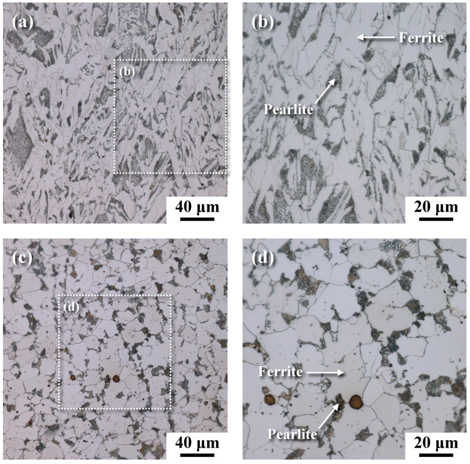
3.1. Metallographs of Base Metals

The metallographs of A106 grade B samples, both cold-drawn (C) and hot-rolled (H), used in this experiment were examined, as shown in Figure 3. The black areas represented the pearlite phase, while the white areas represented the ferrite phase. The grains in the cold-drawn samples were more elongated compared to those in the hot-rolled samples. This variation in grain orientation was attributed to differences in forming temperatures and deformation rates of the pipes. Scanning electron microscopy (SEM) was utilized to analyze defects and cracks induced during the experiments. Figure 4 and Figure 5 show the magnified SEM images of the outer and inner walls of the cold-drawn and hot-rolled samples, respectively. It was observed that there were no crack defects on the outer walls of the samples. However, the number of cracks on the inner wall of the cold-drawn samples was greater than on the inner wall of the hot-rolled samples, with the longest cracks exceeding 100 μm, while most defects were smaller than 10 μm. In contrast, the hot-rolled samples exhibited fewer cracks on the inner wall, with the longest crack not exceeding 50 μm. Figure 6 and Figure 7 present the EBSD and EDS results for the cold-drawn and hot-rolled samples, respectively. The grain orientation distribution maps indicated that the cracks were a mixture of trans-granular and inter-granular types. EDS analysis revealed that the oxides associated with the crack areas were iron oxides. To analyze whether the defects and cracks were influenced by residual strain, HKL Channel 5 software was used to analyze the EBSD data and to obtain the kernel average misorientation (KAM) maps (see Figure 8). The KAM maps were correlated with residual strain; Figure 9 shows that the residual strain on the inner wall of the C sample was higher than that of the H sample. This was attributed to the lower pipe-forming temperature of the C sample, resulting in higher residual strain, which also accounted for the greater number and length of cracks in the C samples [20,21,22].

3.2. Effect of Water Flow on Corrosion

Experiment (1) simulated an environment without water circulation in a power plant. The weight loss per unit area was measured, as illustrated in Figure 9. The relationship between weight loss per unit area and time indicated that the corrosion rate could be divided into three stages. In Stage 1, which occurred during the first approximately 1100 h, the corrosion rate was relatively high due to the absence of protective oxides. During the approximately 1000 h transition to Stage 2, the corrosion rate was significantly lower than in Stage 1. In Stage 3, which more closely resembled actual conditions, the corrosion rate steadily increased over the long-term experiment. The corrosion rates were calculated from the slope of Stage 3. The corrosion rates for the cold-drawn (C) and hot-rolled (H) samples in Stage 3 were 23 μm/year and 19 μm/year, respectively, while in Stage 1, they were 76 μm/year for the cold-drawn samples and 85 μm/year for the hot-rolled samples.

Experiment (2) simulated a period of periodic water circulation in the power plant, where the dissolved oxygen content in the water was higher than in Experiment (1). The trend of weight loss per unit area over time is shown in Figure 10. Similar to Experiment (1), the corrosion rate also exhibited three stages, with the primary corrosion rate occurring in Stage 3 after the long-term test. The corrosion rate in Stage 3 for Experiment (2) was 11 μm/year, which was lower than the corrosion rate observed in Experiment (1).

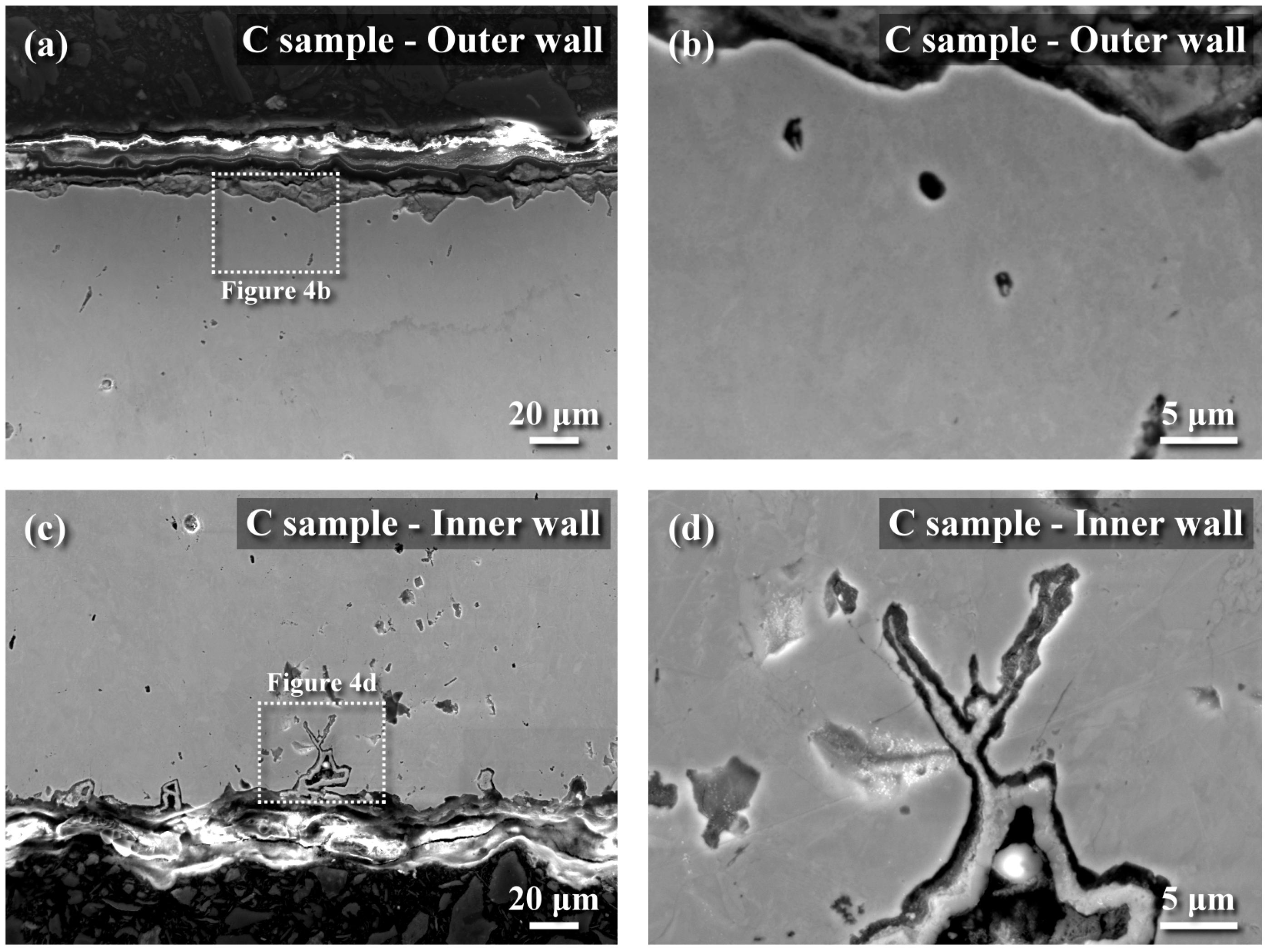
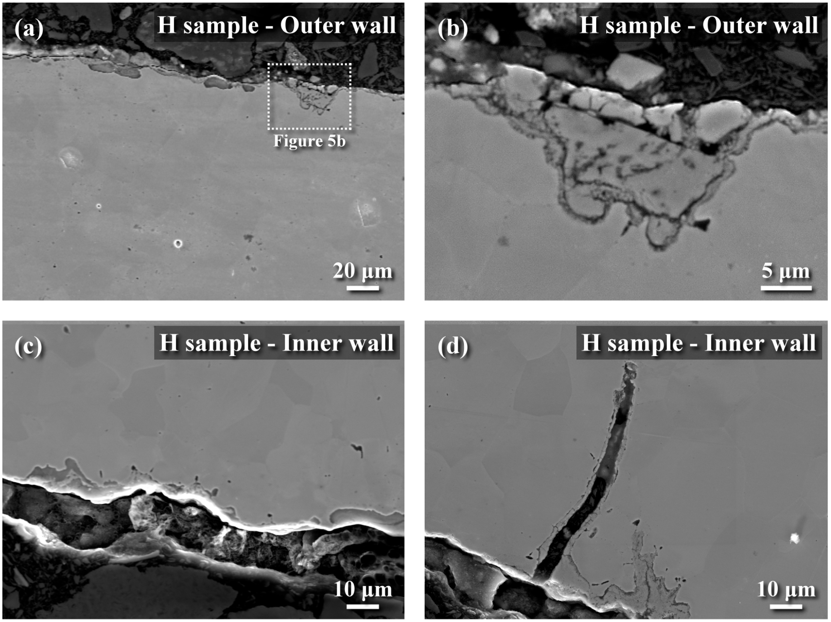
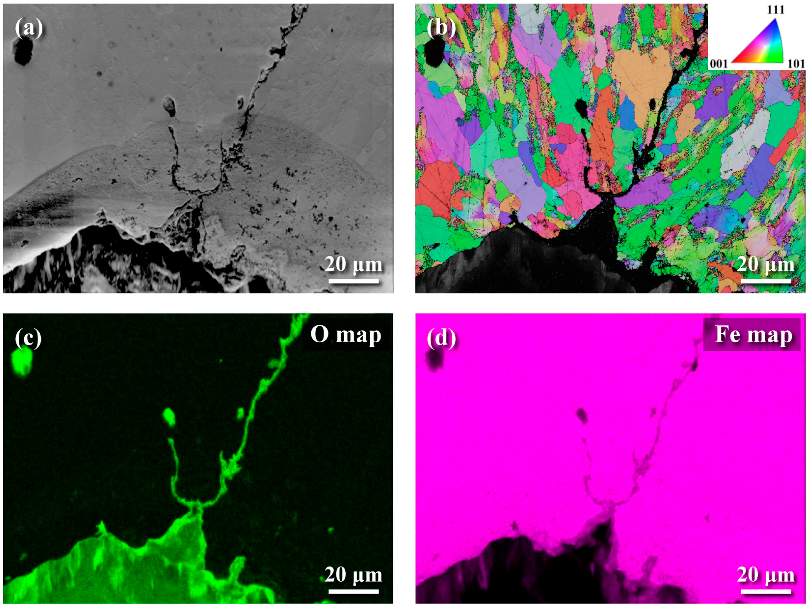
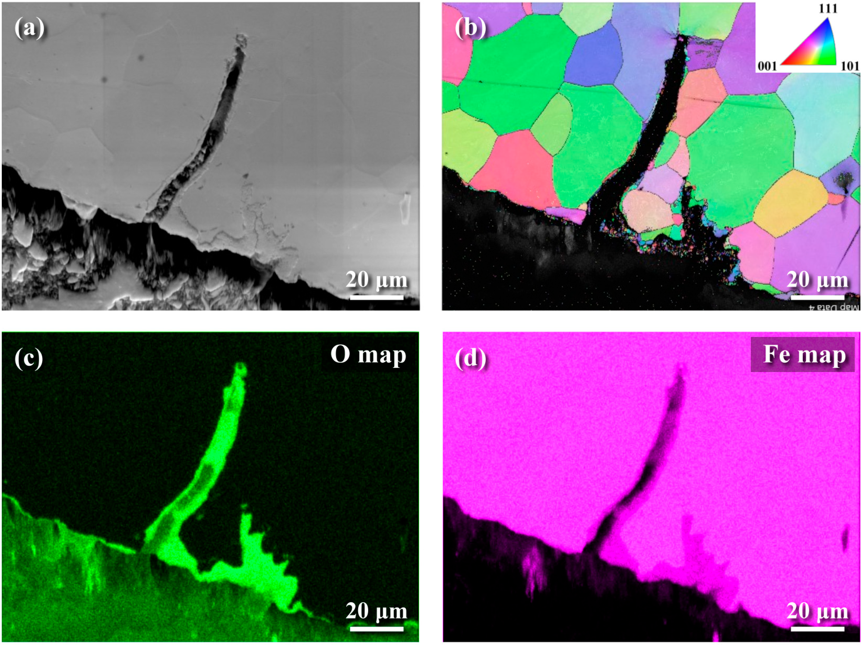
3.3. Corrosion of Partially Immersed Samples

Experiment (3) simulated a scenario where the carbon steel pipes were not completely filled with water in order to observe the corrosion in the interface region. The samples were visually inspected before and after cleaning, as shown in Figure 11. The corrosion in the interface region of the sample (i) was more severe than in other regions. The oxides on sample (a) in the air and those in the interface region of sample (i) could not be removed after cleaning. While most of the oxides in the water region of sample (w) and the interface region of sample (i) were removed, this indicated that the oxides formed in the interface region were similar to those in the air but dissimilar to those in the water. As shown in Figure 11, the interface samples revealed severe corrosion with partial thick oxide layers; the sample submerged in water showed uniform corrosion with a dark appearance; and the sample in air showed corrosion products in localized areas.

The trend of weight loss per unit area as a function of time for the samples in Experiment (3) is shown in Figure 12. The corrosion rate did not exhibit the three stages observed in Experiments (1) and (2). The interface corrosion of sample (i) showed the highest corrosion rate, while the sample in the air exhibited the lowest. The high corrosion rate in the interface region, as shown in Figure 13, was attributed to the surface tension of water at the air–water interface, which formed a thin water film on the carbon steel surface. Yamashita et al. [23] found that the corrosion rates increase when the water film thickness is around 10 μm, leading to more severe corrosion in the interface region. The corrosion rates for samples (a), (i), and (w) in Experiment (3) were 9 μm/year, 93 μm/year, and 88 μm/year, respectively. The corrosion rate of the interface sample (i), 93 μm/year, represented the overall corrosion rate at the air–water interface. Calculating the corrosion rate for the interface region based on the oxide layer thickness yielded 102 μm/year (see Figure 14).

As revealed in

Table 5. Summary of corrosion rate.

Heading	Corrosion Rate (µm/year)	Processes	Water Conductivity(µs/cm)	DissolvedOxygen(ppm)
Experiment (1)	23	Cold-drawn	40.3	0.8
	19	Hot-rolled
Experiment (2)	11	Cold-drawn	0.4~22.3	6~1.72
			The measurements were fluctuating due to periodic water changes.
Experiment (3)	88	Hot-rolled	60.8	2.2
	102	Hot-rolled
	9	Hot-rolled

, The dissolved oxygen levels measured in water for Experiments (1), (2), and (3) were 0.8, 1.72, and 2.2 ppm, respectively, while the water conductivities were 40.3, 22.3, and 60.8 µS/cm, respectively. The corrosion rate of carbon steel in stagnant water was primarily influenced by dissolved oxygen content and ion concentration; higher ion concentrations resulted in higher conductivity. Experiment (2) simulated an environment with periodic water circulation, yielding the highest dissolved oxygen content and the lowest ion concentration. Although Experiment (2) had the highest dissolved oxygen, it exhibited the lowest corrosion rate, indicating that ion concentration significantly affects corrosion rates. Comparing Experiments (1) and (2), the dissolved oxygen in Experiment (2) was much higher, while the ion concentration was much lower, leading to a lower corrosion rate. Thus, it was inferred that ion concentration had a greater effect on corrosion rate than dissolved oxygen when oxygen levels were between 1 and 6 ppm. Therefore, higher ion concentrations were associated with a higher corrosion rate. Comparing Experiments (1) and (3), both the ion concentration and dissolved oxygen were higher in Experiment (3), which resulted in an increased corrosion rate.

Analyzing the composition of the surface oxides on samples helps to understand the corrosion behavior of carbon steel, as metal oxides significantly affect corrosion rates. The metallographs of cross-sections of the interface samples and completely submerged water samples were taken from the right middle part of the samples, which showed the thickest oxide layer. As shown in Figure 11e, the sample reveals the thickest oxide layer in the middle areas. Figure 14a,b show the SEM and EDS results for the surface oxides in the interface region of sample i2 from Experiment (3) and sample H14 from Experiment (1). Figure 14a reveals two distinct microstructures of oxides in sample i2, with the amorphous and more loosely structured oxides identified by EDS being similar to FeOOH or Fe₂O₃, while the denser microstructures are identified as Fe₃O₄. In contrast, the surface oxide of sample H14 in Figure 14b consists solely of the denser Fe₃O₄. XPS analysis was performed on the oxides to verify the EDS results [24,25]. As shown in Figure 15, the results reveal a distinct peak for Fe₃O₄ in sample H14, while the peak for sample i2 falls within the regions of FeOOH and Fe₂O₃. This result supports the finding that in the interface region of sample i2, the sufficient oxygen concentration made it prone to forming FeOOH or Fe₂O₃ [18], while the lack of oxygen in sample H14 resulted in the formation of Fe₃O₄ [18,26].

In this work, due to the absence of protective oxides, the corrosion rate was relatively high during the first stage. The corrosion rate of cold-drawn samples was lower than that of hot-rolled samples at this stage. However, after the long-term test, the overall corrosion rate of cold-drawn samples was higher than that of the hot-rolled samples. The forming processes of the samples influenced the corrosion rate. Cold-drawn samples had a higher surface deformation rate, which increased the homogeneity of the pearlite colonies, as evidenced by SEM and OM observations, and thus improved the corrosion properties in the initial stage [3,27]. Nonetheless, residual stress and surface defects made the oxide films more prone to delamination, leading to a higher corrosion rate for cold-drawn samples in the long-term test.

The passivating action of water plays an important role in corrosion [28], and periodic water circulation helps reduce ion concentration and water conductivity. The corrosion rate is also affected by dissolved oxygen and pH [28]. Although this work did not measure pH, the measurements of dissolved oxygen and conductivity revealed that the corrosion rate increased with higher water conductivity and dissolved oxygen. The influence of ion concentration on the corrosion rate overshadowed that of dissolved oxygen when the dissolved oxygen level was between 1 and 6 ppm.

Dissolved oxygen is also a major parameter in controlling the corrosion of water pipes [29,30]. The results here suggest that pipes filled with purified water had a lower corrosion rate, while the region of the air–water interface exhibited a higher corrosion rate. In the air–water interface region, the water facilitates the transport of ions [30], while oxygen is more easily diffused than in the submerged specimens; therefore, the corrosion rate increases. Additionally, the sufficient oxygen concentration in the interface region led to the formation of less dense oxides, such as FeOOH or Fe₂O₃, while the lack of oxygen in sample H14 resulted in the formation of the denser Fe₃O₄.

The type of general corrosion involves uniform material degradation across the surface, primarily driven by environmental factors such as ion transport, water chemistry, water movement, and dissolved oxygen. To reduce the corrosion rate, the results here suggest that pipes that are completely filled with water will have lower dissolved oxygen; periodic water circulation helps reduce ion concentration and water conductivity.

4. Conclusions

The main observations and conclusions of this research are as follows:

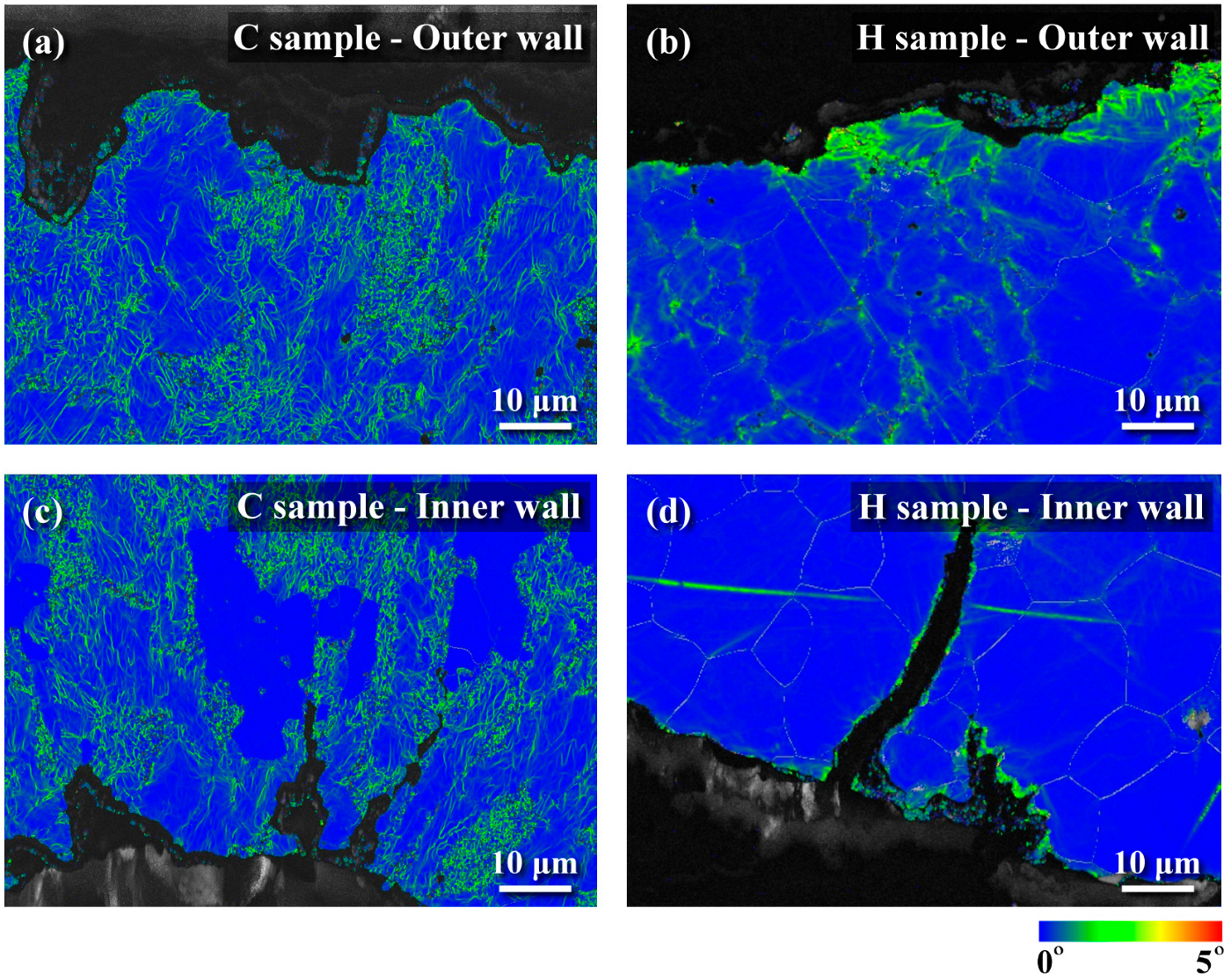
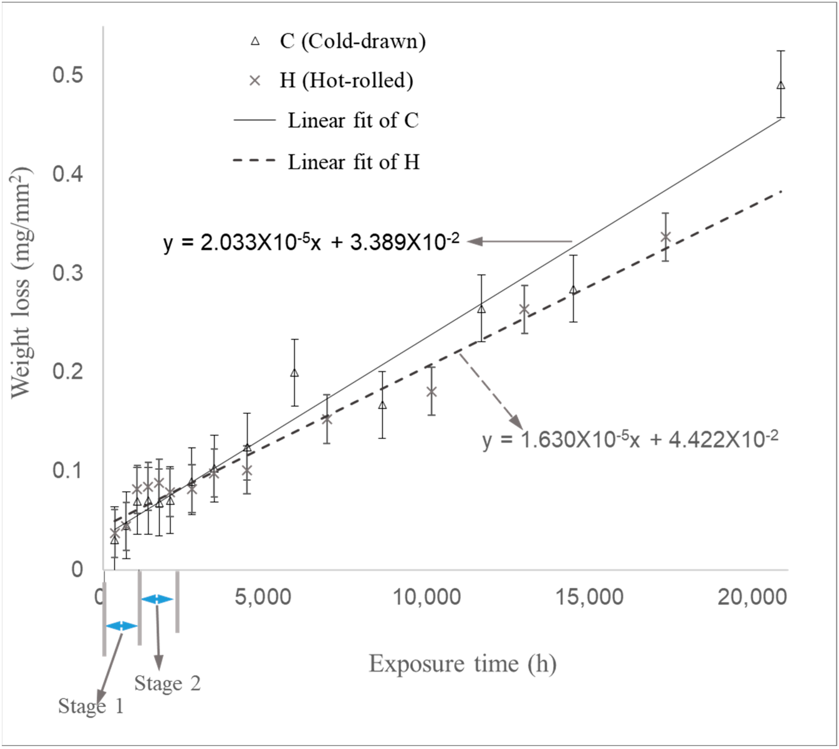
• When the autoclave was filled with stagnant water, the corrosion rates of carbon steel A106 B in stagnant water at 45 °C were 23 μm/year for the cold-drawn samples and 19 μm/year for the hot-rolled samples.
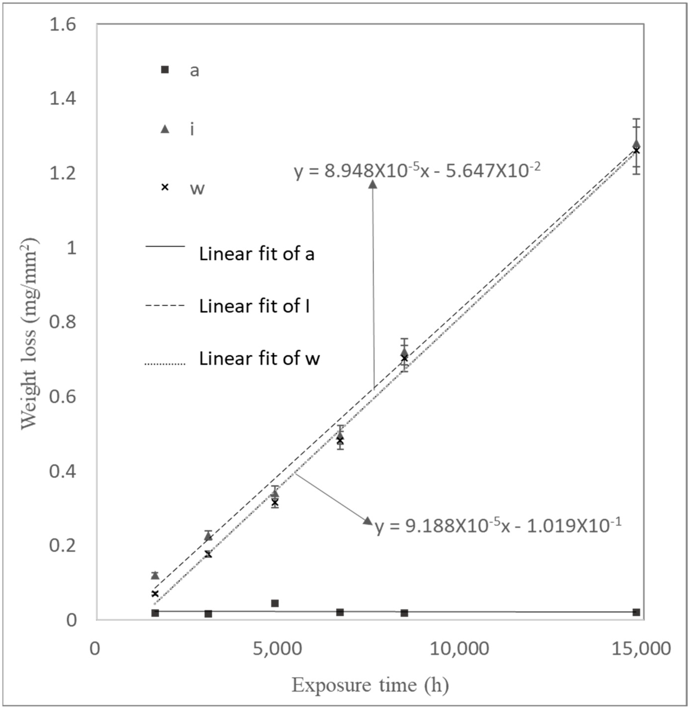
• When the autoclave was partially filled with water and the samples were fully immersed, the corrosion rate for the hot-rolled sample was 88 μm/year.
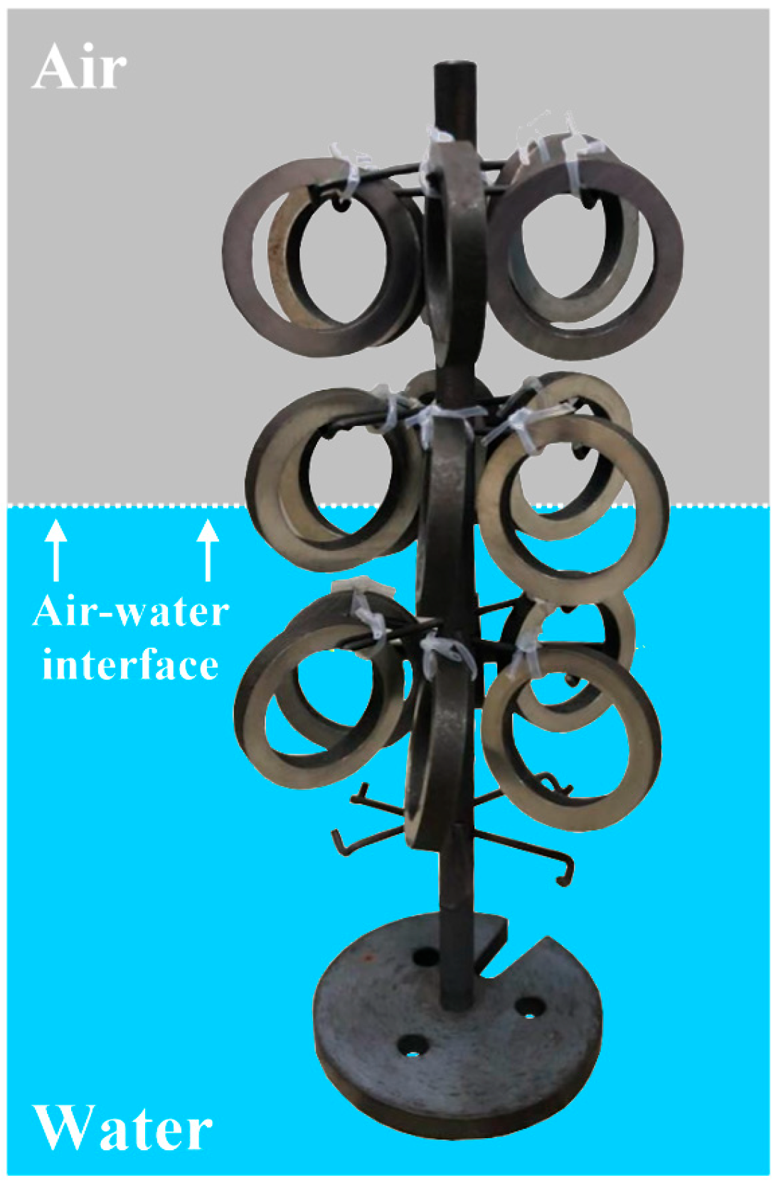
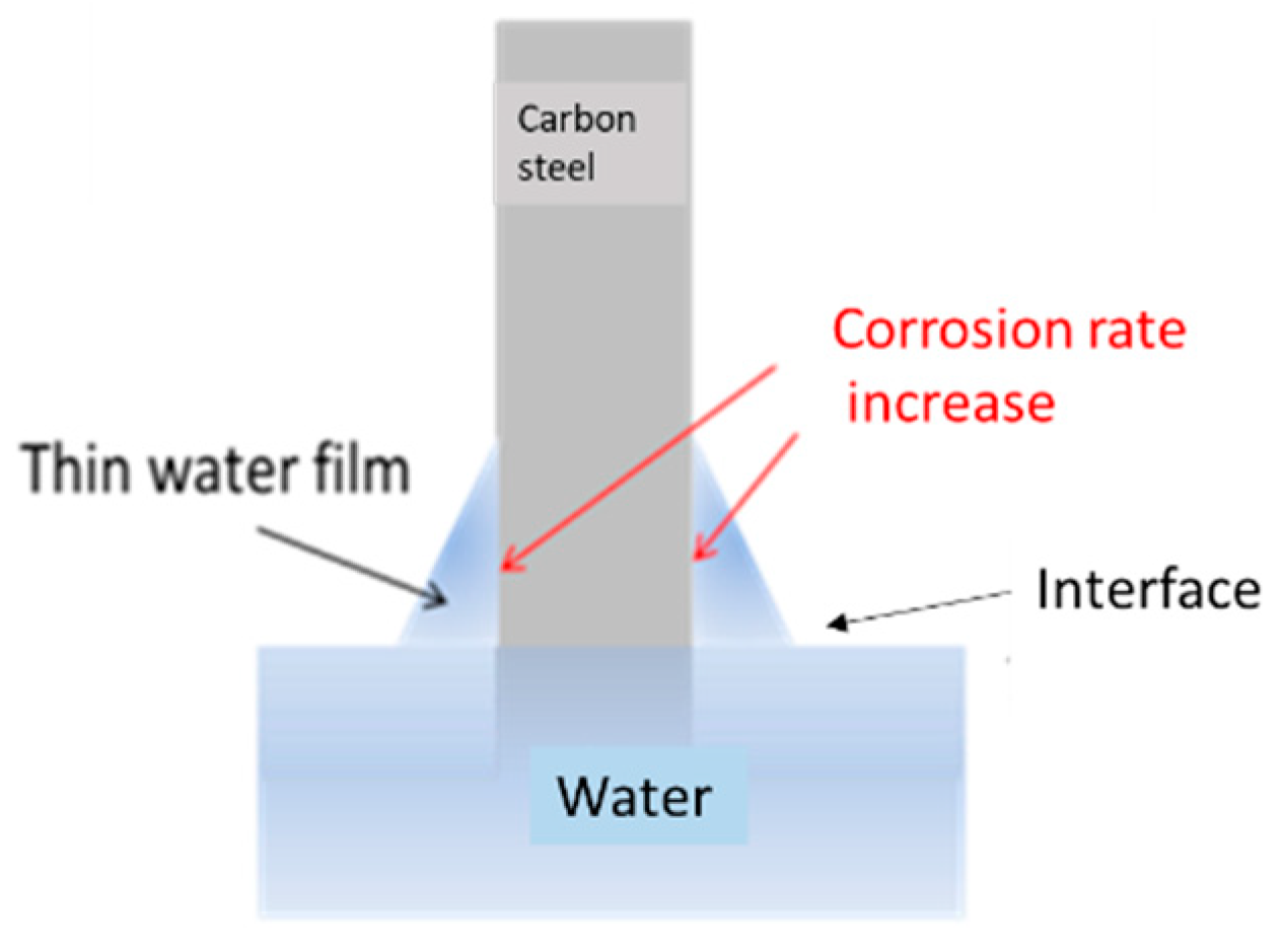
• When the autoclave was partially filled with water and the samples were half-submerged, the corrosion rate for the hot-rolled sample increased to 102 μm/year. In this case, significant corrosion was observed along the air–water interface.
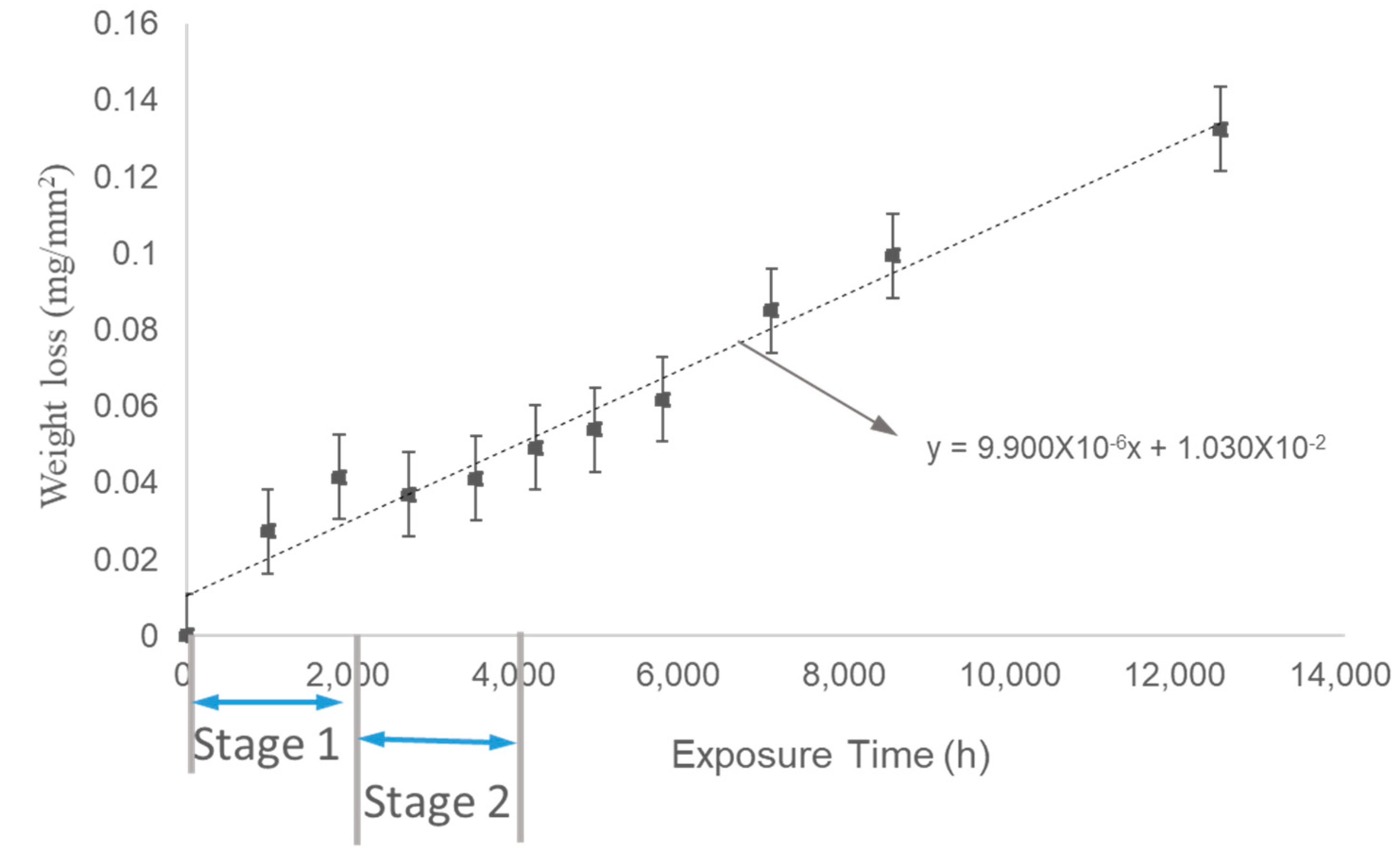
• When the autoclave was filled with stagnant water that was renewed at intervals, the corrosion rate for the cold-drawn sample was 11 μm/year.
• All of the above observations are compatible with higher water conductivity measurements observed at longer water residence times inside the autoclave in combination with higher corrosion along the air–water interfaces.
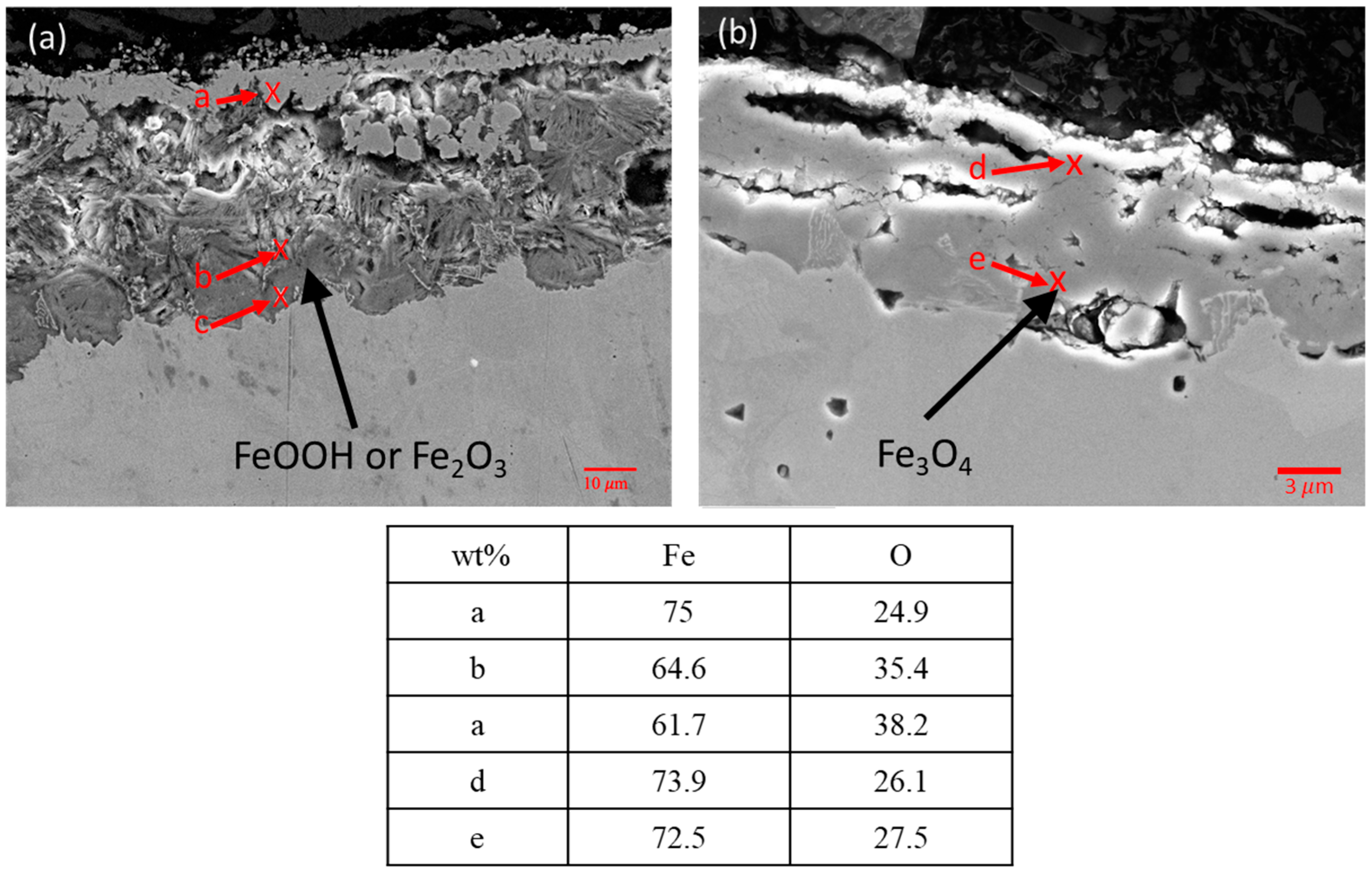
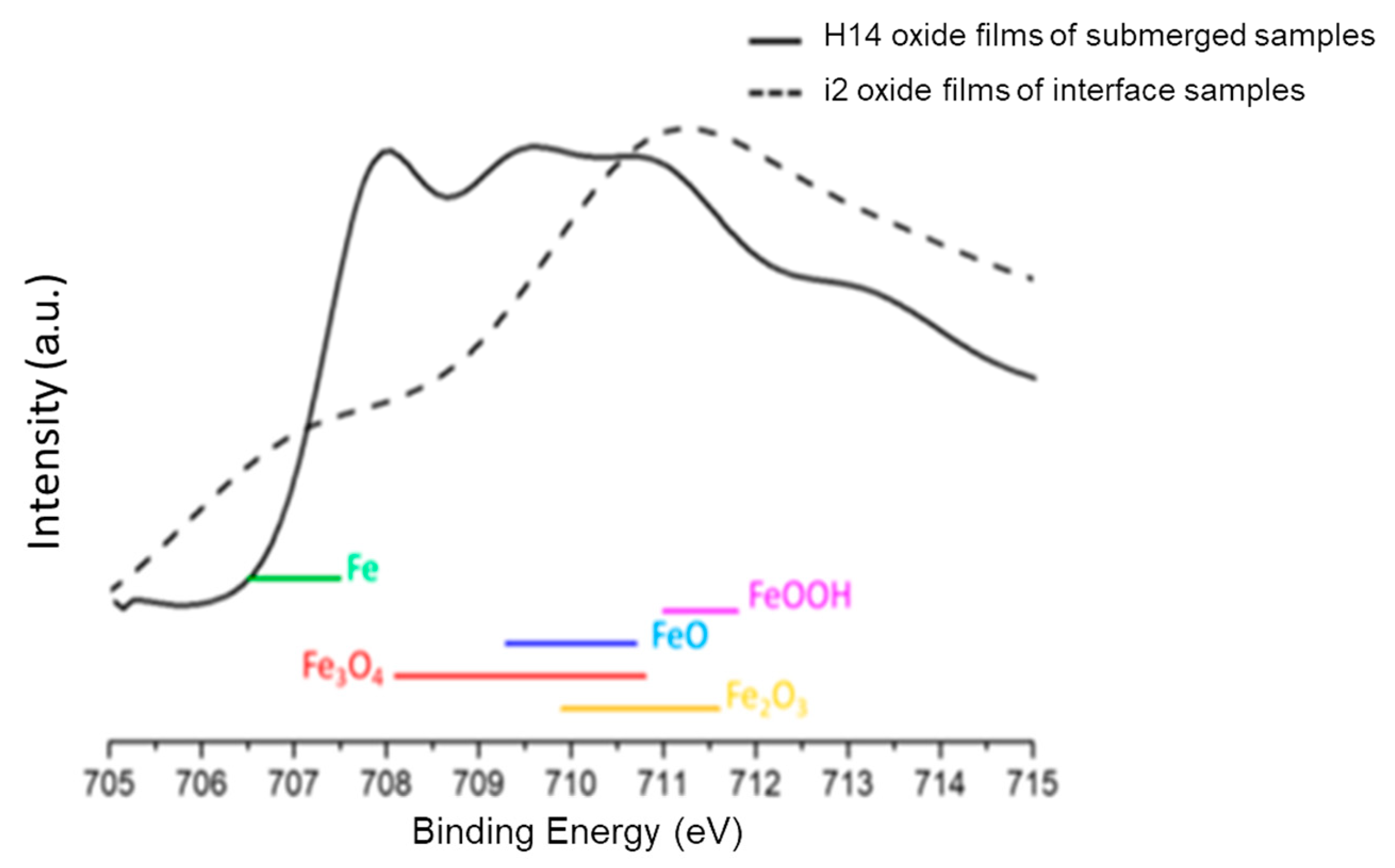
• A sufficient oxygen concentration promotes the formation of FeOOH or Fe₂O₃, while an oxygen-deficient environment favors the formation of Fe₃O₄.

References

1. Rodríguez, M.A. Corrosion control of nuclear steam generators under normal operation and plant-outage conditions: A review. Corros. Rev. 2020, 38, 195–230. [Google Scholar] [CrossRef]
2. Gordon, B.M. Non-environmentally assisted cracking corrosion concerns affecting life extension of light water reactors. Corrosion 2013, 69, 1039–1046. [Google Scholar] [CrossRef] [PubMed]
3. Mendoza, A.R.; Corvo, F. Outdoor and indoor atmospheric corrosion of carbon steel. Corros. Sci. 1999, 41, 75–86. [Google Scholar] [CrossRef]
4. Morcillo, M.; Chico, B.; Diaz, I.; Cano, H.; de la Fuente, D. Atmospheric corrosion data of weathering steels. A Rev. Corros. Sci. 2013, 77, 6–24. [Google Scholar] [CrossRef]
5. Experience, C.O. Degradation and Ageing Programme (CODAP). Available online: https://www.oecd-nea.org/codap (accessed on 1 July 2024).
6. Starosvetsky, D.; Armon, R.; Yahalom, J.; Starosvetsky, J. Pitting corrosion of carbon steel caused by iron bacteria. Int. Biodeterior. Biodegrad. 2001, 47, 79–87. [Google Scholar] [CrossRef]
7. Tang, Z.; Wang, Z.; Lu, Y.; Sun, P. Cause analysis and preventive measures of pipeline corrosion and leakage accident in alkylation unit. Eng. Fail. Analysis. 2021, 128, 105623. [Google Scholar] [CrossRef]
8. May, Z.; Alam, M.K.; Nayan, N.A. Recent Advances in Nondestructive Method and Assessment of Corrosion Undercoating in Carbon–Steel Pipelines. Sensors 2022, 22, 6654. [Google Scholar] [CrossRef]
9. Wasim, M.; Djukic, M.B. External corrosion of oil and gas pipelines: A review of failure mechanisms and predictive preventions. J. Nat. Gas. Sci. Eng. 2022, 100, 104467. [Google Scholar] [CrossRef]
10. Farh, H.M.H.; Ben Seghier, M.E.A.; Taiwo, R.; Zayed, T. Analysis and ranking of corrosion causes for water pipelines: A critical review. NPJ Clean. Water 2023, 6, 65. [Google Scholar] [CrossRef]
11. Seghier, M.E.A.B.; Höche, D.; Zheludkevich, M. Prediction of the internal corrosion rate for oil and gas pipeline: Implementation of ensemble learning techniques. J. Nat. Gas. Sci. Eng. 2022, 99, 104425. [Google Scholar] [CrossRef]
12. Alcántara, J.; de la Fuente, D.; Chico, B.; Simancas, J.; Díaz, I.; Morcillo, M. Marine Atmospheric Corrosion of Carbon Steel: A Review. Materials 2017, 10, 406. [Google Scholar] [CrossRef] [PubMed]
13. Clover, D.; Kinsella, B.; Pejcic, B.; De Marco, R. The influence of microstructure on the corrosion rate of various carbon steels. J. Appl. Electrochem. 2005, 35, 139–149. [Google Scholar] [CrossRef]
14. Tian, H.; Cui, Z.; Ma, H.; Zhao, P.; Yan, M.; Wang, X.; Cui, H. Corrosion evolution and stress corrosion cracking behavior of a low carbon bainite steel in the marine environments: Effect of the marine zones. Corros. Sci. 2022, 206, 110490. [Google Scholar] [CrossRef]
15. Yu, J.; Wang, H.; Yu, Y.; Luo, Z.; Liu, W.; Wang, C. Corrosion behavior of X65 pipeline steel: Comparison of wet–Dry cycle and full immersion. Corros. Sci. 2018, 133, 276–287. [Google Scholar] [CrossRef]
16. Gong, K.; Wu, M.; Liu, G. Comparative study on corrosion behaviour of rusted X100 steel in dry/wet cycle and immersion environments. Constr. Build. Mater. 2020, 235, 117440. [Google Scholar] [CrossRef]
17. Zhao, S.; Jing, Y.; Liu, T.; Zhao, W.; Li, F. Corrosion behavior and mechanism of carbon steel in industrial circulating cooling water system operated by electrochemical descaling technology. J. Clean. Prod. 2024, 434, 139817. [Google Scholar] [CrossRef]
18. Seechurn, Y.; Wharton, J.A.; Surnam, B.Y.R. Mechanistic modelling of atmospheric corrosion of carbon steel in Port-Louis by electrochemical characterisation of rust layers. Mater. Chem. Phys. 2022, 291, 126694. [Google Scholar] [CrossRef]
19. ASTM A106/A106M-18; Standard Specification for Seamless Carbon Steel Pipe for High-Temperature Service. ASTM international: West Conshohocken, PA, USA, 2019.
20. Park, S.A.; Kim, J.G.; He, Y.S.; Shin, K.S.; Yoon, J.B. Comparative study on the corrosion behavior of the cold rolled and hot rolled low-alloy steels containing copper and antimony in flue gas desulfurization environment. Phys. Met. Metallogr. 2014, 115, 1285–1294. [Google Scholar] [CrossRef]
21. Ozgowicz, W.; Grajcar, A.; Kurc-Lisiecka, A. Corrosion Behavior of Cold-Deformed Austenitic Alloys, Corrosion Engineering 2012. Available online: https://www.intechopen.com/chapters/41214 (accessed on 1 July 2024).
22. Dwivedi, D.; Lepkova, K.; Becker, T. Carbon steel corrosion: A review of key surface properties and characterization methods. RSC Adv. 2017, 7, 4580–4610. [Google Scholar] [CrossRef]
23. Yamashita, M.; Nagano, H. Corrosion Potential and Corrosion Rate of Low-Alloy Steel under Thin Layer of Solution. J. Jpn. Inst. Met. Mater. 1997, 61, 721–726. [Google Scholar] [CrossRef]
24. López, D.A.; Schreiner, W.H.; de Sánchez, S.R.; Simison, S.N. The influence of carbon steel microstructure on corrosion layers: An XPS and SEM characterization. Appl. Surf. Sci. 2003, 207, 69–85. [Google Scholar] [CrossRef]
25. Krishna, D.N.G.; Philip, J. Review on surface-characterization applications of X-ray photoelectron spectroscopy (XPS): Recent developments and challenges. Appl. Surf. Sci. Adv. 2022, 12, 100332. [Google Scholar] [CrossRef]
26. King, F.; Padovani, C. Review of the corrosion performance of selected canister materials for disposal of UK HLW and/or spent fuel. Corros. Eng. Sci. Technol. 2011, 46, 82–90. [Google Scholar] [CrossRef]
27. Esmailzadeh, M.; Mousavi, R.; Esfahani, M.M.; Pezzato, L.; Karimi, E. Effect of cold forging on mechanical and corrosion behaviors of carbon steel plate. Int. J. Press. Vessel. Pip. 2022, 198, 104659. [Google Scholar] [CrossRef]
28. Fukaya, Y.; Watanabe, Y. Characterization and prediction of carbon steel corrosion in diluted seawater containing penta borate. J. Nucl. Mater. 2018, 498, 159–168. [Google Scholar] [CrossRef]
29. Jung, H.; Kim, U.; Seo, G.; Lee, H.; Lee, C. Effect of Dissolved Oxygen (DO) on Internal Corrosion of Water Pipes. Environ. Eng. Res. 2009, 14, 195–199. [Google Scholar] [CrossRef]
30. Sarin, P.; Snoeyink, V.L.; Bebee, J.; Jim, K.K.; Beckett, M.A.; Kriven, W.M.; Clement, J.A. Iron release from corroded iron pipes in drinking water distribution systems: Effect of dissolved oxygen. Water Res. 2004, 38, 1259–1269. [Google Scholar] [CrossRef]
Figure 1. CODAP A106 B corrosion failure data, Reprinted from Ref [5].
Metals 14 01444 g001
Figure 2. Schematic of water interface corresponding to samples and experiments.
Metals 14 01444 g002
Figure 3. Metallographs of samples: (a) cold-drawn, (b) the micrograph of boxed area in (a) at a higher magnification, (c) hot-rolled, and (d) the micrograph of boxed area in (c) at a higher magnification.
Metals 14 01444 g003
Figure 4. SEM images of cold-drawn samples (Sample No. C): (a) cross sectional micrograph of out wall, (b) the micrograph of boxed area in (a) at a higher magnification, (c) cross sectional micrograph of inner wall, and (d) the micrograph of boxed area in (c) at a higher magnification.
Metals 14 01444 g004
Figure 5. SEM images of hot-rolled samples (Sample No. H): (a) cross sectional micrograph of out wall, (b) the micrograph of boxed area in (a) at a higher magnification, (c) cross sectional 7micrograph of inner wall, and (d) the micrograph of boxed area in (c) at a higher magnification.
Metals 14 01444 g005
Figure 6. EBSD and EDS images of the inner wall of cold-drawn samples: (a) SEM image, (b) EBSD grain orientation map, (c) EDS oxygen distribution map, and (d) EDS iron distribution map.
Metals 14 01444 g006
Figure 7. EBSD and EDS images of the inner wall of hot-rolled samples: (a) SEM image, (b) EBSD grain orientation map, (c) EDS oxygen distribution map, and (d) EDS iron distribution map.
Metals 14 01444 g007
Figure 8. KAM maps derived from EBSD data of cold-drawn and hot-rolled samples: (a) cold-drawn sample (outer wall), (b) hot-rolled sample (outer wall), (c) cold-drawn sample (inner wall), and (d) hot-rolled sample (inner wall).
Metals 14 01444 g008
Figure 9. Weight loss of samples during Experiment (1) as a function of time.
Metals 14 01444 g009
Figure 10. Weight loss of samples during Experiment (2) as a function of time.
Metals 14 01444 g010
Figure 11. Appearances of the samples in Experiment (3): (a) specimen in air after 2 months of testing, (b) air–water interface specimen after 2 months of testing, (c) specimen completely submerged in water after 2 months of testing, (d) specimen in air after 21 months of testing, (e) air–water interface specimen after 21 months of testing, and (f) specimen submerged in water after 21 months of testing.
Metals 14 01444 g011
Figure 12. Weight loss of samples during Experiment (3) as a function of time.
Metals 14 01444 g012
Figure 13. Schematic diagram of interface corrosion: the relationship between water film thickness and corrosion rate.
Metals 14 01444 g013
Figure 14. SEM images and EDS results of (a) i2, and (b) H14 oxide layers.
Metals 14 01444 g014
Figure 15. XPS spectra of the surface oxide composition.
Metals 14 01444 g015