Effect of Surface Finish on CO₂ Corrosion of Low-Alloy Steel in Simulated Sea Water and Well Environments

Abstract

The study investigates the influence of surface finish on corrosion of a grade API L80 low-alloy steel. Samples of this steel with different surface finishes produced by rough mechanical grinding (RG sample) or by finer polishing (FP sample) have been studied after exposure to corrosive environments. It is found that the dissolution rate is one to two orders of magnitude higher for the RG sample with a rougher surface than for the FP samples with a smoother surface. Scanning electrochemical microscopy shows selective corrosion of the RG sample, while the FP sample undergoes slow uniform corrosion, followed by localized corrosion after long exposure. A detailed analysis of the corrosion process indicates that in a simulated well environment containing Fe²⁺ and Ca²⁺ ions, fast precipitation of CaCO₃ on the rougher surface initially reduces the corrosion rate. However, once a protective scale starts forming on the surface, the effect of surface finish on corrosion resistance becomes less significant. The scale morphology and phase composition vary between the samples with the different surface finishes.

1. Introduction

Fossil fuels continue to be the primary energy source, leading to growing worries about the rising levels of CO₂ emissions and their adverse effects on climate change. Carbon capture and storage (CCS) technology allows the utilization of fossil fuels by capturing CO₂ emissions from significant sources (e.g., power generation, refineries, and industrial applications) and storing them in underground geological formations such as depleted oil and gas reservoirs, thus averting their release into the atmosphere. However, corrosion of the transport and injection pipelines is considered to be a big problem for the economy and the safety of CCS chains [1,2].

Both water drop-out corrosion under the supercritical CO₂ phase and aqueous CO₂ corrosion can occur in the downhole steel tubulars [3]. This can happen when CO₂ injection is stopped intermittently, and the back pressure allows formation water mixed with injected CO₂ to come into contact with the pipelines used for the injection of CO₂ [4]. Furthermore, impurities such as H₂O, O₂, SO_x, NO_x, H₂S, etc. in the captured and injected CO₂ can additionally influence corrosion behavior [1]. To determine and understand the influence of impurities, it is important to initially analyze the corrosion behavior when CO₂ contains no impurities. The reaction of dry CO₂ with formation water results in aqueous corrosion, which is also a critical issue for steel tubulars in the oil and gas industry [5,6].

Low-alloy steel is widely used for production of tubing materials for oil and gas wells and is also considered a possible tubing material for CO₂ storage wells. Corrosion of low-alloy steels due to the CO₂-saturated environment is known to cause pipeline failures with associated increase in operational costs and less sustainable production [5,6]. The dissolution of CO₂ in the source water leads to the formation of carbonic acid (H₂CO₃), which drastically increases the rate of electrochemical reactions between the steel substrate and the aqueous phase, leading to uniform dissolution of Fe and to the development of several crystalline and non-crystalline corrosion products/scales on the steel surface [7,8]. The latter develop due to the interplay between the rate of material dissolution and precipitation of the carbonate and hydroxide phases. Addressing the corrosion problem in these pipelines is vital to ensure the long-term effectiveness and safety of carbon capture and storage technologies for mitigating climate change. Therefore, understanding and controlling parameters that can affect corrosion behavior in varying conditions is the key factor in improving the resistance of the material against deterioration and scale formation.

It has been reported that operational and metallurgical variables directly influence the corrosion rate in CO₂-saturated environments [5,9,10,11,12,13,14,15,16,17,18]. Among different parameters that can affect the corrosion behavior of low-alloy steel in environments containing CO₂, surface roughness is considered to have a significant impact on corrosion rates [19,20,21,22,23,24]. The surface roughness of steel pipelines shipped to coating yards in the oil and gas industry can be in the range 20–50 µm [12]. Furthermore, the pipelines from depleted oil and gas reservoirs to be used for CO₂ injection will have rougher surfaces due to corrosion, different from those in reported lab studies. From a corrosion point of view, irregularities on the surface due to roughness can create microenvironments, changing the local electrolyte chemistry, which can affect the composition and adherence of corrosion scales. Moreover, rough surfaces can also disrupt the boundary layer of fluid flow, altering mass transfer characteristics by bringing more corrosive CO₂ molecules to the metal surface [25,26,27,28]. Despite multiple studies have demonstrated the effect of initial surface roughness on macroscopic corrosion parameters of low-alloy steel in CO₂ environments, its impact on local corrosion behavior and scale formation is not clearly understood.

The paper aims to provide a better understanding of the influence of surface roughness on corrosion rates in CO₂-saturated conditions and to analyze how this relates to species transfer to and from the steel surface, and how this affects material dissolution. This ultimately improves the knowledge of how surface morphology can impact corrosion behavior in simulated sea water and well environments.

2. Materials and Methods

2.1. Material and Surface Preparation

The chemical composition of the grade API L80-0Cr steel used in this work is shown in

Table 1. Chemical composition (wt.%) of the grade API L80-0Cr steel.

C	Cr	Mn	Mo	P	Si	S	Ni	Cu	Fe
0.40	-	1.9	-	0.03	0.45	0.030	0.25	0.35	Bal.

. The samples were received after oil-quenching and tempering. Cylindrical ∅5-mm specimens with a height of 15 mm were cut from the as-received material. The as-cut specimens were mechanically polished to obtain two samples with different surface finishes through (i) rough grinding using a P500 SiC paper (RG sample) and (ii) additional polishing of the mechanically ground surface using P1000 and P4000 SiC papers, followed by polishing using a 1-µm diamond suspension to enable a finely polished surface (FP sample). Grinding and polishing were performed on both flat and curved surfaces of the specimens.

2.2. Surface Roughness Analysis

Surface roughness profiles of the specimens were determined using a CMM-008-Olympus-LEXT laser microscope (Olympus, Tokyo, Japan). Three laser microscopy images were taken for each specimen in randomly selected regions covering an area of 129 µm × 129 µm in each region. Sq representing the root mean square value of heights within these regions was calculated using the SPIP software 4.4.

2.3. Corrosion Measurements

2.3.1. Local Electrochemical Evaluation Using Scanning Electrochemical Microscopy (SECM)

A BioLogic M470 SECM workstation (BioLogic, Seyssinet-Pariset, France) with a three-electrode cell and an electrolyte containing 0.01 M NaCl solution was used in the present study. The microelectrode tip and the sample were applied as working electrodes, while the Pt plate and Ag/AgCl electrode were used as the counter and reference electrodes, respectively. The intermittent contact (ic) SECM mode was used to eliminate signals from surface topography, thus preventing their interference with electrochemical signals. The specimens were maintained at a cathodic potential of −0.85 V vs. Ag/AgCl (approximately −150 mV vs. open circuit potential) to reduce the rate of the oxidation reaction (Fe²⁺ formation). This increased the required time for corrosion initiation and enabled the detection of microphases. Sample generation/tip collection (SG/TC) mode was used by applying a bias potential of +0.60 V vs. Ag/AgCl, so that oxidation of Fe²⁺ to Fe³⁺ ions could occur on the tip surface and consequently generate electrons.

An area of 200 µm × 200 µm on the steel specimens was scanned with a step size of 10 µm in both x- and y-directions to determine the current across the Pt microelectrode tip (I_tip) and to map the distribution of the current. The current distribution maps were collected every 1 h to evaluate the evolution of the corroded surface over time.

2.3.2. Immersion Tests and Analysis of Solution Chemistry

Immersion tests were carried out in a 1.5 L glass cell under simulated sea water containing 1.2 M NaCl solution and 0.015 M NaHCO₃ saturated with CO₂. This simulated sea water was used to mimic a relatively simple and controlled environment with no significant ion interaction or saturation effects. This environment enabled a focused evaluation of the impact of surface roughness on electrochemical activity and, particularly, on the localized corrosion behavior. In order to obtain information on the amount of Fe²⁺ ions in the electrolyte due to material dissolution, ~2 mL of the electrolyte were extracted from the corrosion cell every 30 min using a pipette. These samples were placed in Eppendorf tubes sealed with parafilm and stored in a fridge. Then, for each sample, 1 mL was extracted and diluted in test tubes containing 9 mL of a 2% HNO₃ solution. The ionic concentration was evaluated using inductively coupled plasma–optical emission spectroscopy (ICP-OES). Three calibration solutions (1 ppm, 2 ppm, and 5 ppm of Fe, Cr, Mo, Ni, and Cu each) and one quality control solution (2 ppm of Fe, Cr, Mo, Ni, and Cu each) were systematically prepared to measure the actual concentrations of ions dissolved in the samples. The Fe²⁺ concentration values were calculated taking into account both the dilution with HNO₃ and the “background concentration” measured at t = 0 min, i.e., before the samples were immersed.

2.3.3. Electrochemical Corrosion Measurements

Electrochemical tests were carried out using a standard three-electrode set-up with Ag/AgCl as a reference electrode and a Pt wire as a counter electrode. The electrolyte used for the investigation was a CO₂-saturated simulated well environment with the solution chemistry specified in

Table 2. Ionic composition of the simulated well environment.

Unit	Na+	Cl-	Ca2+	$\mathbf{HC}{\mathbf{O}}_3^{-}$	Fe2+
Mol	1.13	1.43	0.15	0.015	0.0016
Ppm	27,450	53,000	6012	917	90

. This electrolyte contained metallic ions (e.g., Ca²⁺ and Fe²⁺) to mimic more realistic, supersaturated well environments in field applications. The presence of these ions enabled analysis of scales (precipitation of mixed carbonates, e.g., FeₓCaᵧCO₃) and analysis of effects of surface finish on both early-stage corrosion and the formation of protective scales.

Prior to specimen immersion, the electrolyte was deaerated by nitrogen gas bubbling for 12 h. The gas was then changed to CO₂ and the bubbling continued for additional 4 h for saturation. The initial pH of the solution was approximately 5.7, and the experiments were conducted under the CO₂ saturation conditions at 80 °C. The sample was screwed to an in-house designed electrode holder and the electrical resistance was measured using multimeter to verify proper electrical connection. The electrode holder consisted of a threaded stainless steel (SS) rod that was placed inside a hollow glass tube with Teflon ends. Only a screw head of the threaded SS rod was outside one Teflon end. The sample was screwed tightly on the threaded area until the Teflon end, so that SS would not interact with the electrolyte. The working electrode cable of the potentiostat was connected to the SS rod within the electrode holder using crocodile clips, ensuring good electrical connection. One of the flat surfaces of the specimens as well as the curved surface with a total area of 2.55 cm² were exposed to the electrolyte for 94 h.

For the electrochemical experiments, one-hour open circuit potential (OCP) stabilization time was used. Electrochemical impedance spectroscopy (EIS) and linear polarization resistance (LPR) measurements were then carried out after every hour. The EIS measurements were performed by applying an alternating signal with an ±10 mV vs. OCP amplitude in a frequency range between 10 kHz and 10 mHz. Simultaneously, the corrosion potential E_corr and the corrosion resistance were monitored using LPR measurements at 1 h intervals. For the LPR measurements, a potential range of ±10 mV over OCP at a scan rate of 10 mV/min was used, as defined by the ASTM-G59 standard. For potentiodynamic polarization scans, specimens were polarized to ±250 mV vs. OCP and a scan rate of 10 mV/min was applied. All the electrochemical corrosion tests were conducted thrice for better reproducibility.

2.4. X-Ray Diffraction and Scanning Electron Microscopy

The phase composition of the corrosion products induced by CO₂ electrochemical exposure was analyzed using a Bruker D8 Advance X-ray diffractometer (Bruker, Karlsruhe, Germany). The diffractometer was operated at 35 kV and 50 mA using Cr-Kα radiation (λ = 0.22909 nm) in the parallel beam geometry configuration. The X-ray diffractograms were acquired in the angular scattering range 2θ = 30–110°. The Δ2θ step size and the acquisition time per step were 0.03° and 12 s, respectively. The corroded surface morphology and the spatial distribution of chemical elements were evaluated using a Zeiss Sigma 300 scanning electron microscope (Carl Zeiss, Oberkochen, Germany) equipped with an Ultim Max 65 detector (Oxford Instruments, Buckinghamshire, UK) for energy dispersive spectroscopy (EDS) analysis.

3. Results

3.1. Surface Characteristics

The surface profile determined using laser microscopy is shown in Figure 1a,b. It can be seen that the RG sample has a rougher surface, where the average Sq value is measured to be 270 ± 93 nm. On the other hand, the FP sample shows a smooth surface with an average Sq value of 78 ± 12 nm.

3.2. Corrosion Investigations

The corrosion behavior of the samples was determined in two different CO₂-saturated salt solutions: (i) simulated sea water without metallic ions (non-supersaturated solution) and (ii) a simulated well environment containing metallic ions in a supersaturated solution. The effect of these two solutions is presented in the following subsections.

3.2.1. Simulated Sea Water

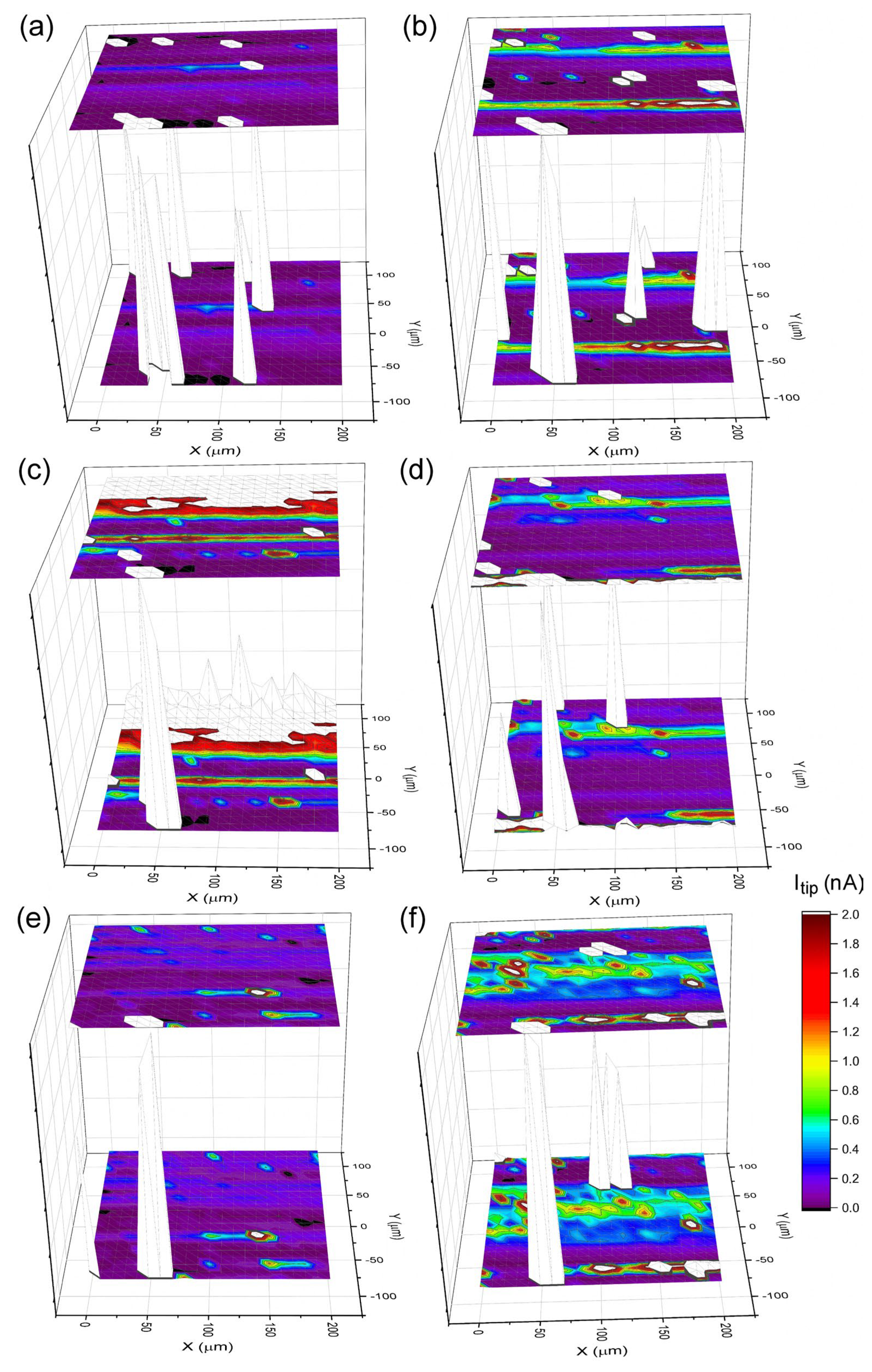
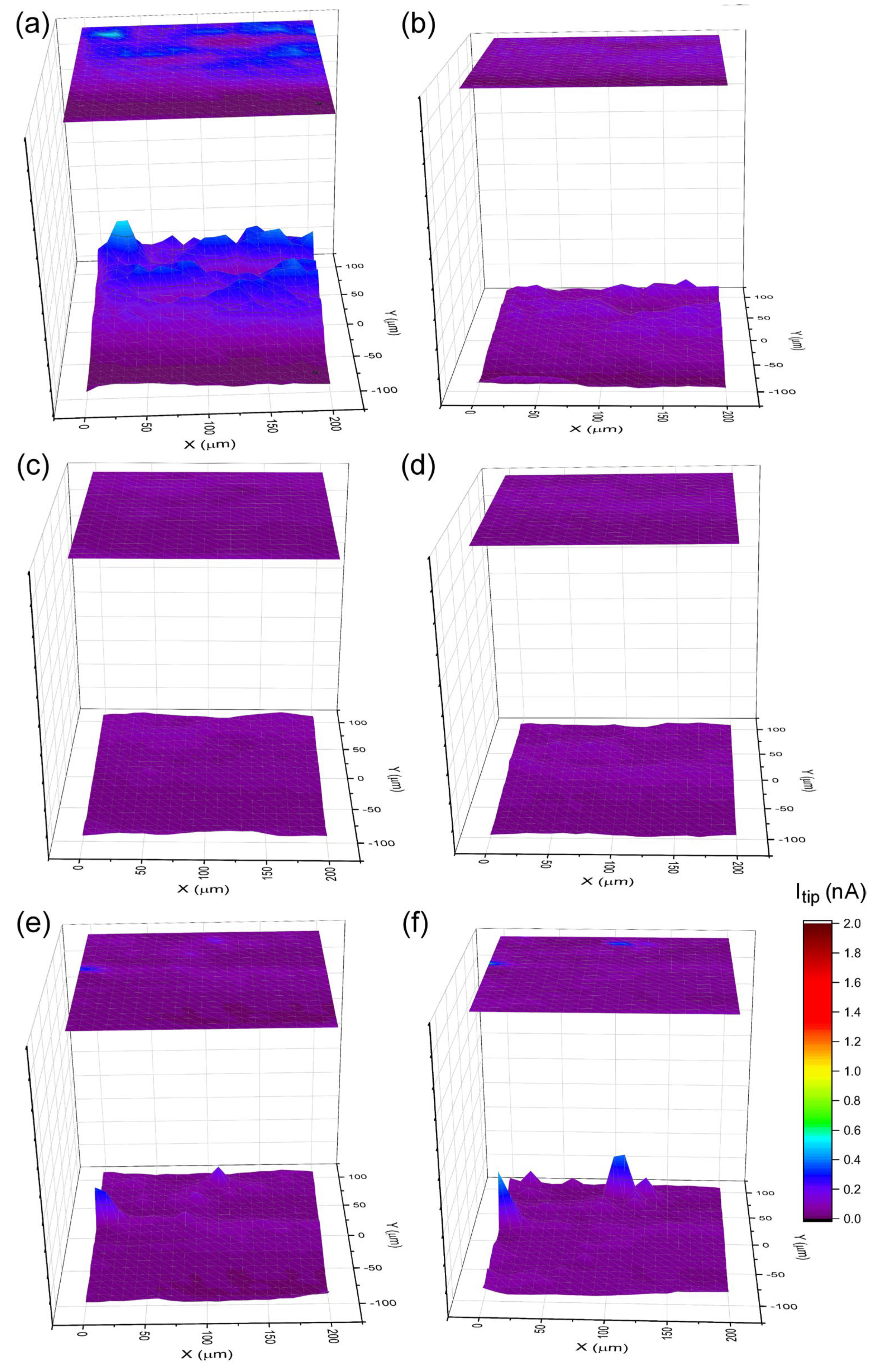
Local Electrochemical Measurements

The ic-SECM current maps for the RG sample and the FP sample are presented in Figure 2 and Figure 3, respectively. The map for the first hour of exposure of the RG sample (Figure 2a) shows selective/localized corrosion generally matching local variations in surface roughness. Some spikes in the current are also observed in Figure 2a. While the majority of these spikes are narrow and most likely represent the measurement noise, the spike close to x = 50 µm and y = −100 µm originates from a larger area and may represent a pit initiation site on the sample surface. This spike is consistently observed throughout the entire exposure period (see Figure 2b–f). With an increase in the exposure time up to 3 h, the current distribution range and the average current over the investigated area increase, while after exposures for more than 3 h, the current distribution range and the average current decrease.

The current distribution map for the FP sample exposed for 1 h (see Figure 3a) shows a more uniform pattern than that observed for the RG sample in Figure 2a. This suggests that the FP sample initially undergoes comparatively uniform corrosion as opposed to selective/localized corrosion of the RG sample. An increase in the exposure time up to 4 h (see Figure 3b–d) does not result in significant changes in the distribution of current, which implies a low corrosion rate. Localized electrochemically active sites appear on the FP sample after 5 h of exposure. However, measured currents for this sample are still less significant compared to those for the RG sample. The presence of the localized sites suggests that the long-term exposure of the FP sample can result in selective corrosion.

The average current defined by the total current measured over the investigated area divided by the total number of points is one to two orders of magnitude less for the FP sample compared to the RG sample. More specifically, the average current for the RG sample is in the range 1–5 nA for the entire test duration, while the average current for the FP sample is in the range 0.05–0.2 nA. The lower average current for the FP sample implies a lower corrosion rate for the FP sample compared to that for the RG sample.

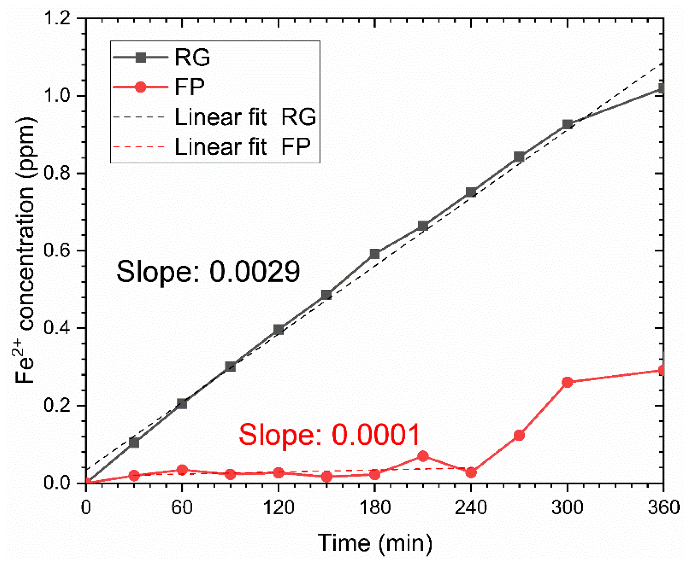
Dissolution Kinetics

The concentration of Fe²⁺ ions obtained due to dissolution of Fe during the immersion test and measured using ICP-OES is shown in Figure 4 as a function of exposure time. The Fe²⁺ concentration in the electrolyte is found to be much higher for the RG sample than for the FP sample, thus providing evidence of greater corrosion of the rougher-surface sample. Slopes seen in Figure 4 suggest that the corrosion rate for the RG sample is one order of magnitude higher than that for the FP sample. Although the corrosion rate for the FP sample is very low within the first 4 h of exposure, the initially smooth surface can roughen during this 4 h exposure, resulting in an increased dissolution rate for durations between 4 h and 6 h (see Figure 4).

3.2.2. Simulated Well Environment

Potentiodynamic Polarization Test

Figure 5 illustrates the results of potentiodynamic polarization tests conducted in CO₂-saturated electrolyte at 80 °C, providing valuable insights into the electrochemical behavior of the studied samples. The cathodic polarization curves reveal a series of slope changes across the overpotential range, which correspond to transitions between different dominant cathodic reactions. This behavior indicates shifts in the reaction mechanisms depending on the applied potential.

Within the small cathodic overpotential range (50–150 mV vs. OCP), a notable difference in reaction kinetics is observed between the two samples. For the FP sample, the cathodic reaction is predominantly controlled by activation polarization (through H₂ reduction reaction), suggesting that the reaction rate is controlled by the energy barrier for the electrochemical process. In contrast, the cathodic reaction for the RG sample appears to be diffusion-controlled within this potential range, indicating that the rate is limited by the transport of reactants (e.g., dissolved ${\mathrm{HCO}}_3^{-} \mathrm{or} {\mathrm{CO}}_3^{2-}$ species) to the electrode surface. Despite these differences in reaction mechanisms, the overall current density across the cathodic potential region does not differ significantly between the two samples. This suggests that, while the governing processes differ, the net cathodic reaction rates remain similar in the present experiment.

For the anodic polarization behavior, the reaction kinetics at anodic overpotentials display similar trends for the RG and FP samples. This indicates that the anodic dissolution process, which involves the oxidation of iron to form ferrous ions (Fe²⁺), is largely unaffected by the differences in the surface finish.

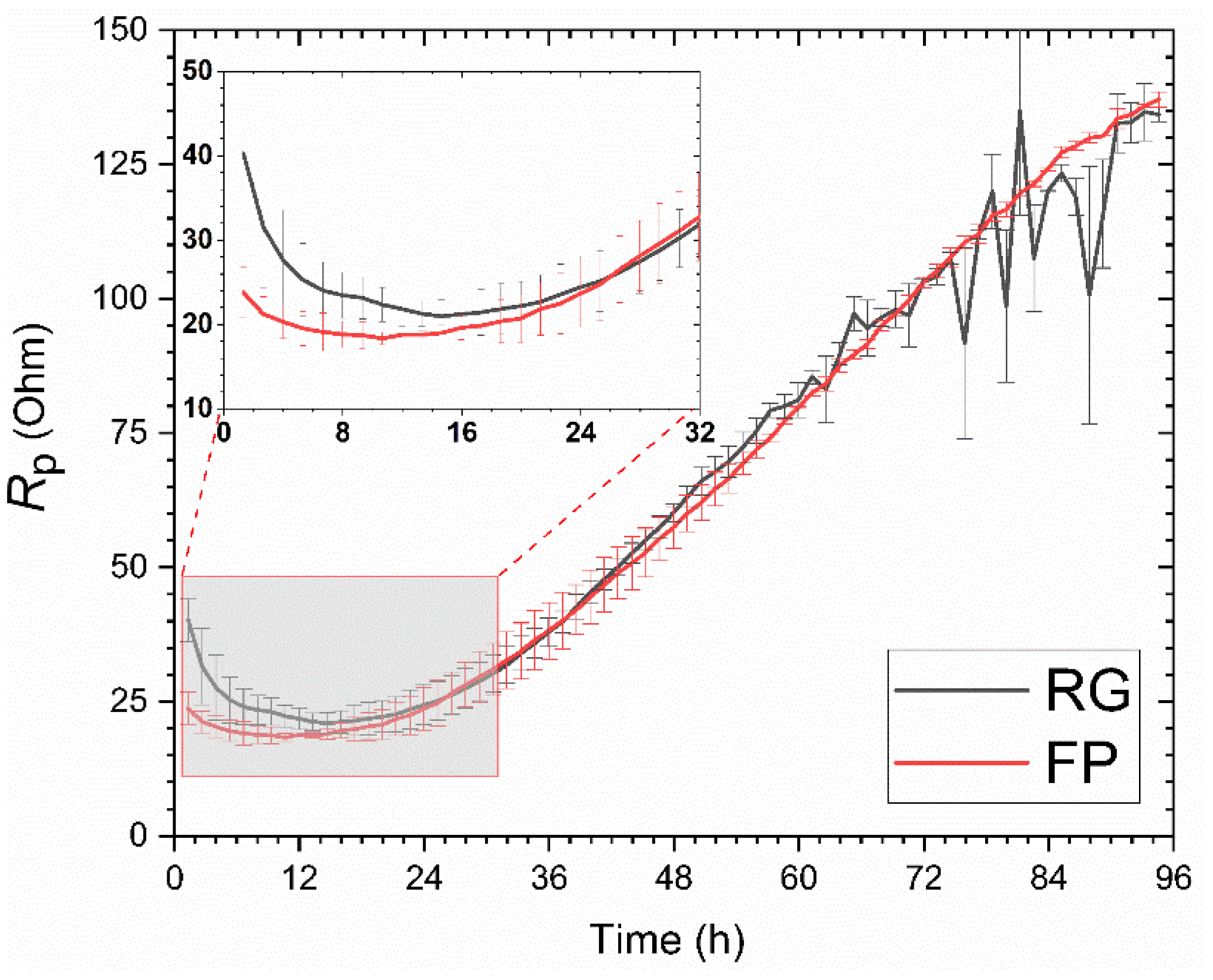
Linear Polarization Resistance Measurements

The linear polarization resistance R_p of the samples tested in the simulated well environment is presented in Figure 6. The LPR results can be divided into two main stages: I—decreasing trend (material dissolution); and II—increasing trend (scaling). The results show that the corrosion resistance for a short period of exposure (stage I) is dependent on the surface finish. However, the influence of surface finish on the corrosion resistance becomes less significant after the development of protective scale.

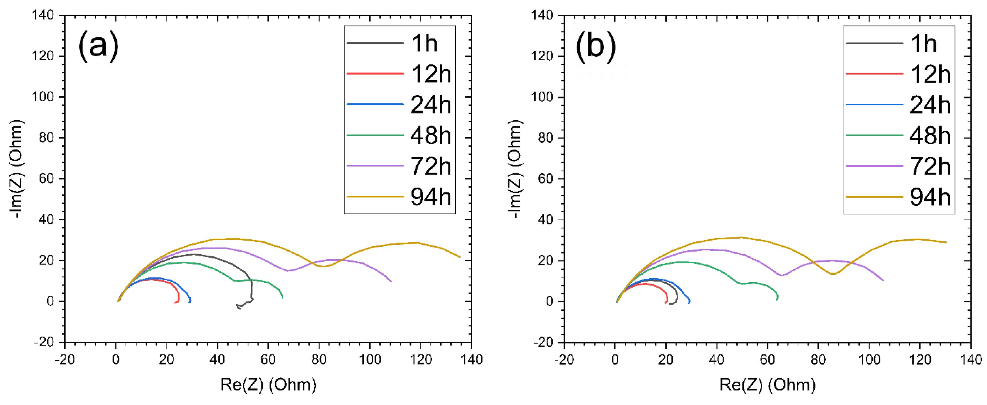
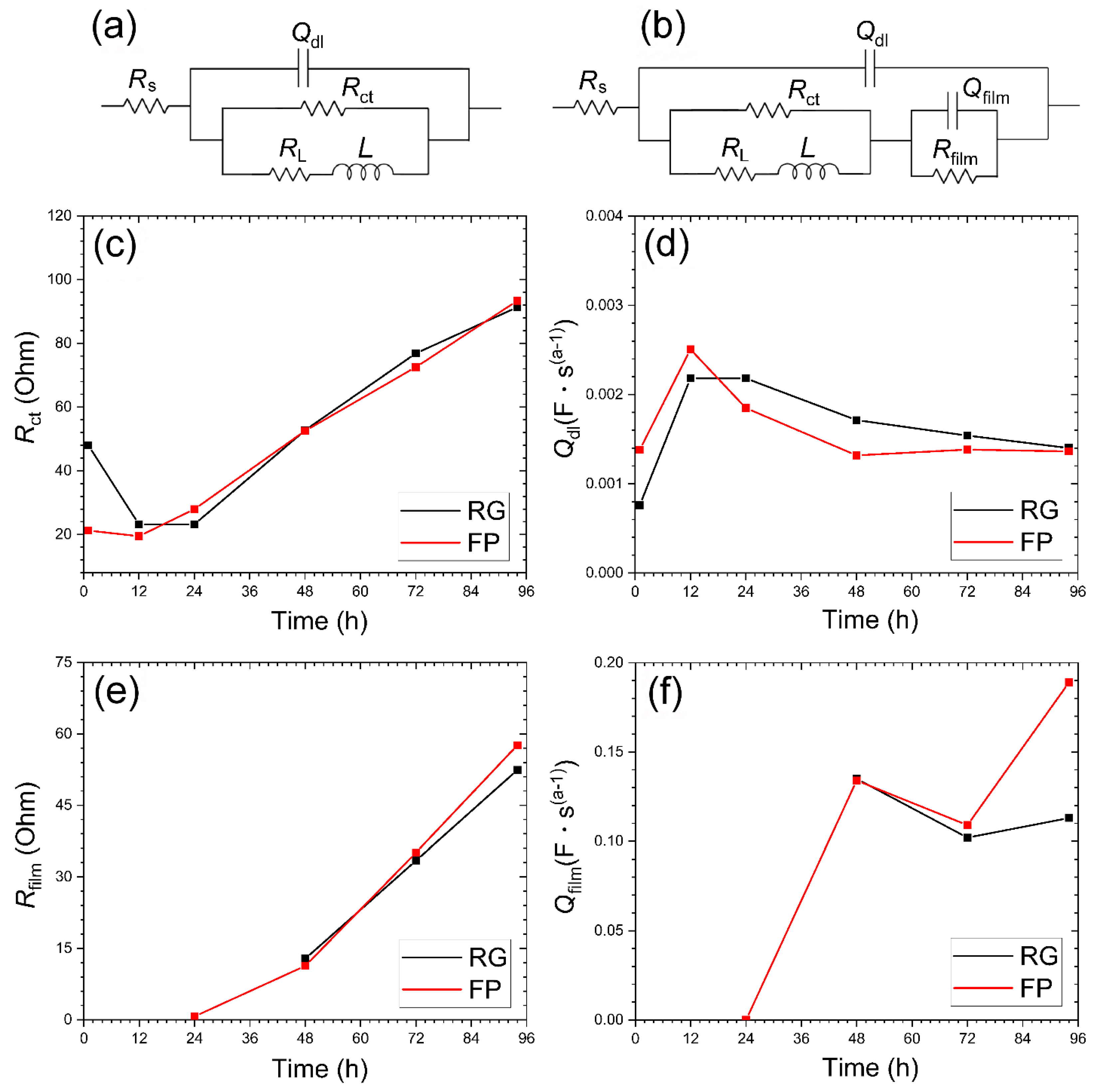
Electrical Impedance Spectroscopy Analysis

Figure 7 shows impedance spectra corresponding to the corrosion behavior presented in the form of Nyquist plots for the samples after every 12 h or 24 h of exposure in the simulated well environment. These plots indicate the interfacial electrical resistance between the specimens and CO₂-saturated electrolyte, thereby providing information about the CO₂ corrosion behavior and scaling.

The samples show one semicircular loop after exposures for up to 24 h and two semicircular loops after longer exposures. The large loop observed at high to medium frequencies (HF-MF) represents the material resistance to charge transfer, while the second loop at low frequencies (LF) is characteristic of either intermediate reactions or scaling behavior. The low-frequency inductive behavior arises either due to intermediate reactions or improper connections. Since inductive behavior was not observed at higher exposure times, it cannot be related to poor connection and is, thus, considered to be related to intermediate reactions. The larger diameter of the semi-circle at HF-MF for the RG sample suggests better resistance of the sample to corrosion, which is consistent with the LPR measurements shown in Figure 6. With an increase in exposure time, the diameter of the semi-circle initially decreases due to an increase in the material dissolution rate. However, at longer exposures, a non-ideal capacitive loop corresponding to the protective scale is observed instead of an inductive pseudo-capacitive loop.

To quantify the corrosion behavior, the EIS spectra for corroding steel substrates can further be analyzed using numerical fitting combined with the equivalent electrical circuit similar to the equivalent circuit used in our previous work [18]. The Nyquist curves with the inductive pseudo-capacitive loop at LF were fitted using the equivalent circuit shown in Figure 8a, while the Nyquist curves with the capacitive loop at LF (corresponding to the protective scale development) were fitted using the equivalent circuit shown in Figure 8b. The Nyquist curves were fitted with the equivalent circuits using a Randomize + Simplex function. The fitting parameter χ²/|z| in Equation (1) is less than 0.1, thus indicating a good fit.

$${\displaystyle \frac{{\chi }^2}{\left|z\right|}}={\displaystyle \sum }_{i=1}^n{\displaystyle \frac{{\left|Z_{meas}\left(i\right)-Z_{Simul}\left(f_i,param\right)\right|}^2}{\left|Z_{meas}\left(i\right)\right|}}$$

(1)

The evolution of the individual parameters obtained after fitting (see Figure 8c–f) demonstrates the effect of surface roughness on corrosion behavior. For each sample, resistance to charge transfer R_ct initially decreases, followed by a continuous increase (see Figure 8c). The Q_dl curve representing the capacitance of the electrical double layer (Figure 8d) shows an initial steady increase, followed by a decreasing trend. For both samples, the film resistance R_film (Figure 8e) shows an increasing trend, which suggests the development and growth of the corrosion scale. In contrast, the Q_film curves representing the film capacitance (see Figure 8f) do not show clear trends for each sample. Some variations in R_film and Q_film are observed between the RG and FP samples exposed for more than 72 h.

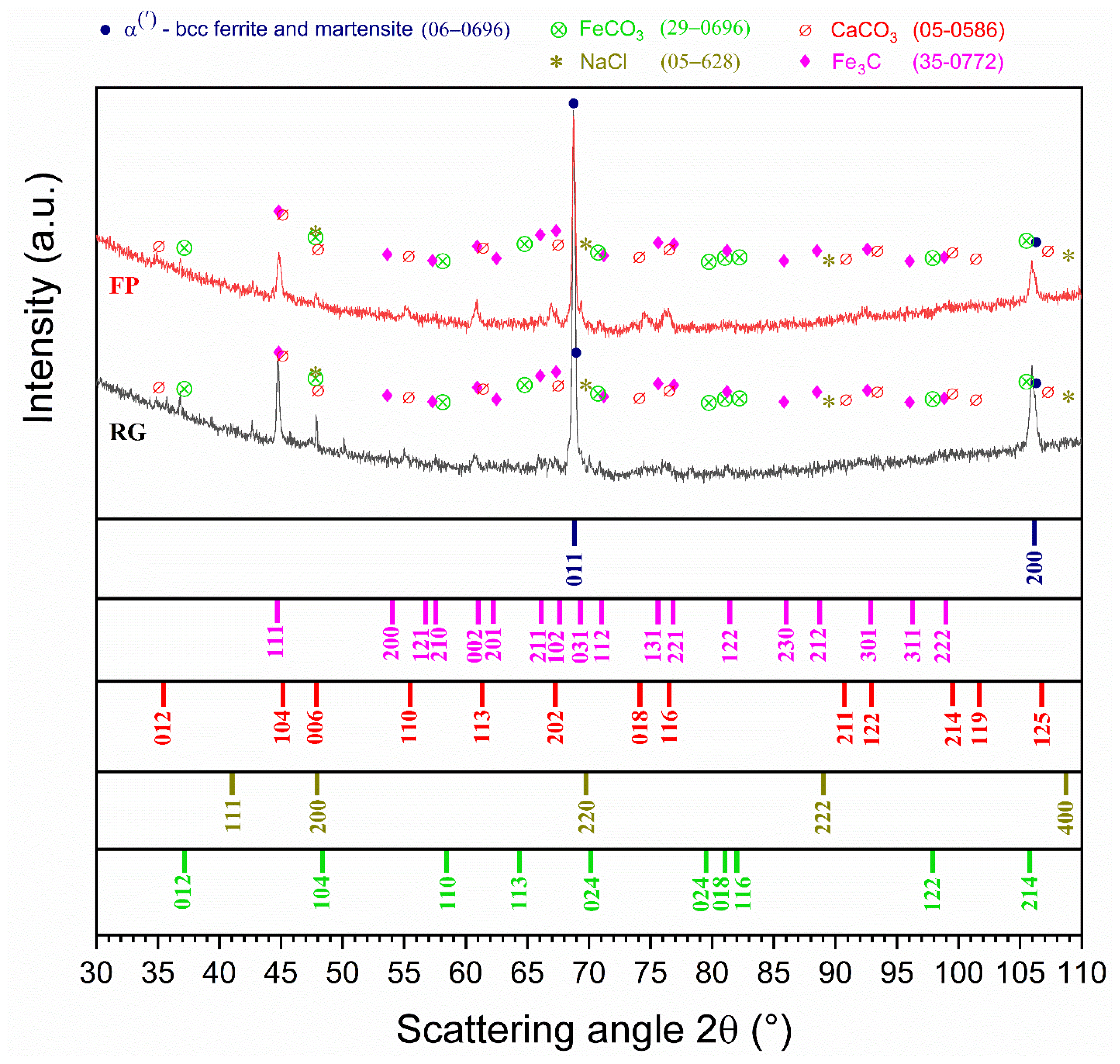
Surface Analysis Using X-Ray Diffraction and SEM-Based Techniques

The X-ray diffractograms for the samples after 94 h of exposure to the electrolyte are presented in Figure 9. The diffractograms reveal the presence of different crystalline corrosion products on the sample surface. The corrosion scale comprises siderite FeCO₃ and calcite CaCO₃ together with cementite Fe₃C on each sample. It is also seen that both the FeCO₃ and the CaCO₃ peaks for the samples are slightly shifted from their respective reference lines, suggesting the presence of mixed Fe_xCa_yCO₃ carbonates. The X-ray diffractograms also show lower intensities of the FeCO₃ and the CaCO₃ peaks for the FP sample compared to those for the RG sample.

The morphology of the corroded samples is presented in Figure 10a,c, where directional features are clearly seen. These directional features are a sign of selective corrosion, and they seem to be deeper in the RG sample (Figure 10a) than in the FP sample (Figure 10c), thus implying that the surface finish affects the morphology of the corroded surface. Elemental maps obtained using EDS show the presence of O, Ca, Fe, and C on the corroded surface (see Figure 10b,d). The observation of all these elements suggests mixed carbonates developed during corrosion, while the observation of regions with only Fe and O suggests cracking and delamination of the corrosion scales formed on the steel surface. Localized corrosion in the form of mesa corrosion attack (pits) can also be observed on the surface of the samples.

4. Discussion

The effect of the initial surface finish of a low-alloy steel on corrosion in the CO₂-saturated salt solution and simulated well environment chemistry is elucidated in this work using electrochemical methods and surface characterization techniques. The results obtained indicate that the CO₂ corrosion behavior is strongly influenced by the initial surface finish of the material. The effect of surface finish on the CO₂ corrosion behavior of the grade API L80-1Cr steel is discussed henceforth.

The corrosion behavior in the simulated sea water solution containing only Cl^- ions, evaluated using SECM and immersion tests, suggests that the corrosion rate for the RG sample is initially almost one order of magnitude higher than that for the FP sample having a smoother surface (see Figure 4). The higher corrosion rate for the RG sample is attributed to the combined effect of an increased surface area exposed to the corrosive environment and faster transfer of electrochemically active species induced by the increased surface roughness. These observations are in agreement with several other studies of CO₂ corrosion in steels [24,29,30,31,32,33].

On the other hand, LPR measurements for the material in the simulated well environment show that the RG sample has higher resistance to corrosion than the FP sample during stage I (see Figure 6). Under these conditions, the concentration of metallic ions supersedes the ionic concentration for carbonate supersaturation, resulting in precipitation of metal carbonates as a semi-protective barrier [17,18,34]. The higher corrosion resistance for the RG sample during the first 24 h of exposure to the simulated well environment is probably due to the precipitation of the semi-protective calcium-rich mixed Fe_xCa_yCO₃ phase [18], which reduces the permeability of ions through the formation of a porous scale. The sluggish ion transport is also evident from the observation of small cathodic overpotentials for the RG sample (see Figure 5). The presence of a higher frequency of nucleating sites due to the rougher surface of the RG sample can account for enhanced precipitation of mixed Fe_xCa_yCO₃ carbonates. The higher Q_dl values (Figure 8d) for the first 12 h of exposure of the FP sample suggest smaller surface areas of anodic sites leading to corrosion. However, as this scale is porous and continuously dissolving, the material dissolution rate is high. This conclusion is supported by the observation of a faster drop in corrosion resistance for the RG sample compared to the FP sample. The larger slope of the Q_dl curve (Figure 8d) for the RG sample compared to the FP sample is probably due to a combination of two factors: (i) an increase in surface roughness due to corrosion; and (ii) the dissolution of porous mixed Fe_xCa_yCO₃ carbonates. The development of surface roughness causes an increase in the corrosion rate, which is considered to be the main reason for the initial reduction in R_ct.

The roughness-sensitive corrosion rate influences scaling behavior and scale morphology. During stage II (scaling), the formation of semi-protective mixed Fe_xCa_yCO₃ corrosion products blocks the anodic sites (thus decreasing Q_dl) and leads to an increase in R_ct (see Figure 8) [35]. During the material dissolution, the lower corrosion rate for the FP sample results in enhanced Fe dissolution and thus FeCO₃ supersaturation is reached faster than that for the RG sample. This leads to faster precipitation of the mixed Fe_xCa_yCO₃ products. Therefore, stage II is observed earlier in the FP sample. The faster scale development for the FP sample evident from the LPR and Nyquist plots is also confirmed by the corresponding R_film vs. time curve in Figure 8e. For both samples, the R_film shows an increasing trend, suggesting the development and growth of the corrosion scale, while the Q_film curves (see Figure 8f) suggest competition between scale development and disintegration. During stage II, the change in R_p values with exposure time is similar for both samples with different initial roughness. This indicates that after the initial material dissolution, the corrosion properties of the exposed samples are almost independent of the initial surface finish of the material. This result is consistent with those obtained by Bai et al. [36], who reported that after the complete formation of the protective scale, the corrosion rate of J55 carbon steel depended on the formed corrosion scale rather than on the initial surface roughness.

Nevertheless, the phase composition of the formed scales varies depending on the surface finish. This is evident from the X-ray diffractrograms, which show lower intensities of the carbonate peaks for the FP sample compared to those for the RG sample (see Figure 9). One possible reason for the much higher intensities of the peaks for mixed Fe_xCa_yCO₃ products in the X-ray diffractrograms for the RG sample is the initial precipitation on the rougher sample, as discussed in the previous sections. On the other hand, the FP sample undergoes more dissolution, resulting in a greater amount of residual Fe₃C together with the presence of carbonates in the corrosion scale. In contrast, the dissolution in the RG sample is less pronounced; thus, the scale comprises more carbonates and less cementite, as observed in the XRD results. The variation in the phase composition of the scale results in variations in scale properties (see Figure 8), where small variations in R_film and Q_film are observed between the samples exposed for at least 72 h. The lower Q_film and R_film values for the RG sample than those for the FP sample suggest a thicker yet porous corrosion film (see Figure 8e,f). On the other hand, the high Q_film and R_film values for the FP sample imply that the corrosion scale was more compact and thinner (see Figure 8e,f). This is also evident from the SEM micrographs in Figure 10a,c, which show a much more cracked and disintegrated corrosion scale on the surface of the RG sample compared to that of the FP sample.

Also, varying corrosion modes are observed for the samples with different surface finishes. The rougher surface of the RG sample shows both selective corrosion and localized corrosion from the beginning of exposure to the corrosive environment (see Figure 3), and the scale formed on this sample showed greater local dissolution. The evidence of local dissolution of the formed scale is also seen in the SEM image for the RG sample (Figure 10a). This dissolution results in large error bars for the R_p values obtained after exposures beyond 72 h (see Figure 6). The FP sample undergoes slow uniform corrosion, followed by selective corrosion upon further exposure (see Figure 2). The occurrence of selective corrosion of this sample during extended exposures is probably due to different local pH values resulting from gradual surface roughening in the corrosive environment, which disrupts the mass transfer boundary layer, thus affecting the rates of transfer of electroactive and chemical species [37].

The results discussed above clearly show that the surface finish influences the initial corrosion resistance and corroded morphology as well as scale morphology and phase composition. However, the influence of surface finish on corrosion resistance becomes less significant after the development of the semi-protective scale. Further studies are required to evaluate the influence of surface finish on scale adherence under dynamic conditions.

5. Conclusions

The influence of surface finish on CO₂ corrosion and scaling in simulated sea water and well environments has been investigated in this work for low-alloy steel. The following conclusions are derived from this study:

• The surface finish influences the inherent resistance of the material to CO₂ corrosion. The FP sample with a smooth surface exposed to simulated sea water shows higher initial corrosion resistance. On the other hand, the presence of metallic ions in the simulated well environment enables faster precipitation of calcium carbonates, which lowers initially high corrosion rates for the RG sample with a rougher surface.
• The higher rate of corrosion for the RG sample in the simulated well environment allows faster supersaturation of FeCO₃ and results in a faster formation of a semi-protective Fe_xCa_yCO₃ scale compared to that of the FP sample. Although the phase composition of the scale is different in the samples with different surface finishes, the influence of the observed differences in the phase composition on corrosion resistance is not significant.
• While the RG sample with the rougher surface shows severe selective corrosion after short-term exposures, the FP sample initially shows slow uniform corrosion, followed by selective corrosion in small areas after longer exposures.

References

1. Barker, R.; Hua, Y.; Neville, A. Internal corrosion of carbon steel pipelines for dense-phase CO2 transport in carbon capture and storage (CCS)—A review. Int. Mater. Rev. 2017, 62, 1–31. [Google Scholar] [CrossRef]
2. Yevtushenko, O.; Bettge, D.; Bohraus, S.; Bäßler, R.; Pfennig, A.; Kranzmann, A. Corrosion behavior of steels for CO2 injection. Process Saf. Environ. Prot. 2014, 92, 108–118. [Google Scholar] [CrossRef]
3. Pfennig, A.; Wolf, M.; Kranzmann, A. Corrosion and corrosion fatigue of steels in downhole ccs environment-a summary. Processes 2021, 9, 594. [Google Scholar] [CrossRef]
4. Neel, G.; Millet, C.; Greenwood, J.; Rodriguez, D.; Simon, L.; Lima, L. Material Selection for Anthropogenic CO2 Injection, Mechanical and Corrosion Behavior of Steels Under CO2 with Impurities. In Proceedings of the 16th International Conference on Greenhouse Gas Control Technologies, GHGT-16, Lyon, France, 23–27 October 2022; pp. 1–19. [Google Scholar] [CrossRef]
5. Kane, R.D. Corrosion in Petroleum Production Operations. In ASM Handbook: Corrosion: Environments and Industries; ASM International: Almere, The Netherlands, 2006; pp. 922–966. [Google Scholar] [CrossRef]
6. Popoola, L.T.; Grema, A.S.; Latinwo, G.K.; Gutti, B.; Balogun, A.S. Corrosion problems during oil and gas production and its mitigation. Int. J. Ind. Chem. 2013, 4, 35. [Google Scholar] [CrossRef]
7. Moiseeva, L.S. Carbon dioxide corrosion of oil and gas field equipment. Prot. Met. 2005, 41, 76–83. [Google Scholar] [CrossRef]
8. Kermani, M.B.; Morshed, A. Carbon Dioxide Corrosion in Oil and Gas Production—A Compendium. Corrosion 2003, 59, 659–683. [Google Scholar] [CrossRef]
9. Dwivedi, D.; Lepková, K.; Becker, T. Carbon steel corrosion: A review of key surface properties and characterization methods. RSC Adv. 2017, 7, 4580–4610. [Google Scholar] [CrossRef]
10. Gupta, K.K.; Haratian, S.; Mishin, O.V.; Ambat, R. CO2 corrosion resistance of low-alloy steel tempered at different temperatures. Corros. Sci. 2024, 232, 112027. [Google Scholar] [CrossRef]
11. Nešić, S. Key issues related to modelling of internal corrosion of oil and gas pipelines—A review. Corros. Sci. 2007, 49, 4308–4338. [Google Scholar] [CrossRef]
12. Li, W.; Xiong, Y.; Brown, B.; Kee, K.E.; Nesic, S. Measurement of wall shear stress in multiphase flow and its effect on protective FeCO3 corrosion product layer removal. In Proceedings of the CORROSION 2015, Dallas, TX, USA, 15–19 March 2015; pp. 1–15. [Google Scholar]
13. Tanupabrungsun, T.; Brown, B.; Nesic, S. Effect of pH on CO2 Corrosion of Mild Steel at Elevated Temperatures. In Proceedings of the CORROSION 2013, Orlando, FL, USA, 17–21 March 2015; pp. 1–11. [Google Scholar]
14. López, D.A.; Pérez, T.; Simison, S.N. The influence of microstructure and chemical composition of carbon and low alloy steels in CO2 corrosion. A state-of-the-art appraisal. Mater. Des. 2003, 24, 561–575. [Google Scholar] [CrossRef]
15. Gupta, K.K.; Haratian, S.; Gupta, S.; Mishin, O.V.; Ambat, R. The effect of cooling rate-induced microstructural changes on CO2 corrosion of low alloy steel. Corros. Sci. 2022, 209, 110769. [Google Scholar] [CrossRef]
16. Gupta, K.K.; Yazdi, R.; Styrk-Geisler, M.; Mishin, O.V.; Ambat, R. Effect of microstructure of low-alloy steel on corrosion propagation in a simulated CO2 environment. J. Electrochem. Soc. 2022, 169, 111504. [Google Scholar] [CrossRef]
17. Gupta, K.K.; Haratian, S.; Mishin, O.V.; Ambat, R. The impact of minor Cr additions in low alloy steel on corrosion behavior in simulated well environment. Npj Mater. Degrad. 2023, 7, 1–12. [Google Scholar] [CrossRef]
18. Haratian, S.; Gupta, K.K.; Larsson, A.; Abbondanza, G.; Bartawi, E.H.; Carlà, F.; Lundgren, E.; Ambat, R. Ex-situ synchrotron X-ray diffraction study of CO2 corrosion-induced surface scales developed in low-alloy steel with different initial microstructure. Corros. Sci. 2023, 222, 111387. [Google Scholar] [CrossRef]
19. Poulson, B. Mass transfer from rough surfaces. Corros. Sci. 1990, 30, 743–746. [Google Scholar] [CrossRef]
20. Tantirige, S.; Trass, O. Mass transfer at geometrically dissimilar rough surfaces. Can. J. Chem. Eng. 1984, 62, 490–496. [Google Scholar] [CrossRef]
21. Postlethwaite, J.; Lotz, U. Mass transfer at erosion corrosion roughened surfaces. Can. J. Chem. Eng. 1988, 66, 75–78. [Google Scholar] [CrossRef]
22. Cornet, I.; Lewis, W.; Kappesser, R. Effect of surface roughness on mass transfer to a rotating disc. Trans. Inst. Chem. Eng. 1969, 47, 222–226. [Google Scholar]
23. Gabe, D.; Makanjuola, P. Enhanced mass transfer using roughened rotating cylinder electrodes in turbulent flow. J. Appl. Electrochem. 1987, 17, 370–384. [Google Scholar] [CrossRef]
24. Al-Khateeb, M.; Barker, R.; Neville, A.; Thompson, H. An experimental and theoretical investigation of the influence of surface roughness on corrosion in CO2 environments. J. Corros. Sci. Eng. 2017, 20, 1–29. [Google Scholar]
25. King, C.V.; Howard, P.L. Heat Transfer and Diffusion Rates at Solid- Liquid Boundaries. Ind. Eng. Chem. 1937, 29, 75–78. [Google Scholar] [CrossRef]
26. Brennan, W.C. Mass Transfer in Turbulent Pipe Flow. The Effect of Surface Roughness. Ph.D. Thesis, University of Toronto, Toronto, ON, Canada, 1963. [Google Scholar]
27. Fogg, G.; Morse, J. Development of a new solvent-free flow efficiency coating for natural gas pipelines. In Proceedings of the Rio Pipeline Conference & Exposition 2005, IBP1233, Rio de Janeiro, Brazil, 17–19 October 2005. [Google Scholar]
28. Nordsveen, M.; Nešić, S.; Nyborg, R.; Stangeland, A. A Mechanistic Model for Carbon Dioxide Corrosion of Mild Steel in the Presence of Protective Iron Carbonate Films—Part 1: Theory and Verification. Corrosion 2003, 59, 443–456. [Google Scholar] [CrossRef]
29. Asma, R.B.A.N.; Yuli, P.A.; Mokhtar, C.I. Study on the effect of surface finish on corrosion of carbon steel in CO2 environment. J. Appl. Sci. 2011, 11, 2053–2057. [Google Scholar] [CrossRef]
30. Nesic, S.; Postlethwaite, J.; Thevenot, N. Superposition of diffusion and chemical reaction controlled limiting currents—Application to CO2 corrosion. J. Corros. Sci. Eng. 1995, 1, 1–14. [Google Scholar]
31. Mahato, B.K.; Voora, S.K.; Shemilt, L.W. Steel pipe corrosion under flowconditions-I. An isothermal correlation for a mass transfer model. Corros. Sci. 1968, 8, 173–180. [Google Scholar] [CrossRef]
32. Ma, W.; Wang, H.; Wang, Y.; Neville, A.; Hua, Y. Experimental and simulation studies of the effect of surface roughness on corrosion behaviour of X65 carbon steel under intermittent oil/water wetting. Corros. Sci. 2022, 195, 109947. [Google Scholar] [CrossRef]
33. Silverman, D.C. The rotating cylinder electrode for examining velocity-sensitive corrosion—A review. Corrosion 2004, 60, 1003–1023. [Google Scholar] [CrossRef]
34. Li, H.; Li, D.; Zhang, L.; Bai, Y.; Wang, Y.; Lu, M. Fundamental aspects of the corrosion of N80 steel in a formation water system under high CO2 partial pressure at 100 °C. RSC Adv. 2019, 9, 11641–11648. [Google Scholar] [CrossRef]
35. Rizzo, R.; Ambat, R. Effect of initial CaCO3 saturation levels on the CO2 corrosion of 1Cr carbon steel. Mater. Corros. 2021, 72, 1076–1090. [Google Scholar] [CrossRef]
36. Bai, H.; Cui, X.; Wang, R.; Lv, N.; Yang, X.; Li, R.; Ma, Y. Effect of Surface Roughness on Static Corrosion Behavior of J55 Carbon Steel in CO2-Containing Geothermal Water at 65 °C. Coatings 2023, 13, 821. [Google Scholar] [CrossRef]
37. Al-Khateeb, M.A.M.J. An Experimental and Modelling Study of The Effect of Surface Roughness on Mass Transfer and Corrosion in CO2 Saturated Oilfield Environments, The University of Leeds. 2019. Available online: http://etheses.whiterose.ac.uk/24279/ (accessed on 28 July 2022).
Figure 1. Surface profiles of the RG sample (a) and the FP sample (b).
Metals 15 00302 g001
Figure 2. Maps showing the distribution of current Itip in 3D (lower parts) and 2D (upper parts) for the RG sample exposed to the simulated sea water for different durations: (a) 1 h, (b) 2 h, (c) 3 h, (d) 4 h, (e) 5 h, and (f) 6 h.
Metals 15 00302 g002
Figure 3. Maps showing the distribution of current Itip in 3D (lower parts) and 2D (upper parts) for the FP sample exposed to the simulated sea water for different durations: (a) 1 h, (b) 2 h, (c) 3 h, (d) 4 h, (e) 5 h, and (f) 6 h.
Metals 15 00302 g003
Figure 4. Concentration profiles of Fe2+ obtained from the immersion experiments after different exposures in simulated sea water.
Metals 15 00302 g004
Figure 5. Potentiodynamic polarization curves obtained for the samples exposed to the simulated well environment.
Metals 15 00302 g005
Figure 6. Linear polarization resistance Rp for the samples exposed to the simulated well environment.
Metals 15 00302 g006
Figure 7. Nyquist plots for the RG sample (a) and for the FP sample (b) after exposures in the simulated well environment for 1 h to 94 h.
Metals 15 00302 g007
Figure 8. Equivalent circuits used for fitting the EIS results without the corrosion scale (a) and with the corrosion scale (b) as well as individual parameters of equivalent circuits as a function of exposure time in the simulated well environment: (c) resistance to charge transfer Rct; (d) double-layer capacitance Qdl; (e) film resistance Rfilm for transfer of ions through porosities; (f) film capacitance Qfilm.
Metals 15 00302 g008
Figure 9. X-ray diffractograms for the samples after exposure in the simulated well environment for 94 h.
Metals 15 00302 g009
Figure 10. SEM micrographs (a,c) and elemental maps (b,d) obtained from the sample surface after exposure in the simulated well environment for 94 h: (a,b) RG sample; (c,d) FP sample.
Metals 15 00302 g010