Spectroscopical Characterization of Copper–Iron (Cu-Fe) Alloy Plasma Using LIBS, ICP-AES, and EDX

Abstract

In this present work, we demonstrated a spectral characterization of copper–iron (Cu-Fe) alloy using optical emission spectroscopy. The Cu-Fe alloy plasma was generated on the target sample surface by directing the laser pulse of Q-switched Nd: YAG of the second harmonic (2ω) with a 532 nm optical wavelength. The optical emission spectrum was acquired using five miniature spectrometers that lie within the wavelength range of 200–720 nm. The emission plasma was characterized by validating the local-thermodynamical equilibrium (LTE) as well as optically thin (OT) plasma condition. In addition, the LTE condition was verified using the McWhirter criterion, and the OT condition was validated by comparing theoretically calculated intensity ratios with experimental ones. Plasma parameters, including electron number density as well as plasma temperature, were estimated. In the first stage, the plasma temperature was estimated using the Boltzmann-plot method and the two-line method. The average calculated value of the plasma temperatures were 8014 ± 800 K and 8044 ± 800 K using the Boltzmann-plot and two-line methods, respectively. In the second stage, electron number density was estimated using the Saha–Boltzmann equation and stark-broadening method (SBM). The average number density calculated from the SBM was $2.73\times {10}^{16} {\mathrm{cm}}^{-3}$ and from the Saha–Boltzmann equation was $3.9\times {10}^{16} {\mathrm{cm}}^{-3}$, showing a good agreement. Finally, the comparative compositional analysis was performed using CF-LIBS, Boltzmann Intercept Method, EDX, and ICP-AES, which showed good agreement with that of the standard composition.

1. Introduction

Numerous metallic materials utilized in the industry are blends of various kinds of metals because pure metals have distinctive properties for many industrial applications [1]. For instance, copper (Cu) has various excellent characteristics, such as corrosion resistance, electrical and thermal conductivity, ductility, and softness [2]. However, pure metals can have undesirable characteristics that will destroy the application if used alone. Copper is a weak metal in this situation. Work-hardening methods can be used to strengthen it, but another option to make it stronger is to incorporate additional metals, such as iron. Iron is ductile and malleable, just like copper. It can be stretched without breaking and has good conductivity and tensile strength. Iron, however, is corrosive because it oxidizes to generate rust when exposed to oxygen and water. Iron may boost the tensile strength and corrosion resistance of copper alloys without affecting their inherent conductivity, which is one of the key advantages of adding iron to copper alloys [3,4,5]. High tensile strength and thermal conductivity, resistance to corrosion, and high electrical conductivity are all features of copper–iron (Cu-Fe) master alloys [6]. Combined with various copper alloys, such as aluminum brass, and bronze alloys, this master alloy serves as a grain refiner [7]. Low-alloyed coppers’ mechanical characteristics are often enhanced [8].

Laser-Induced Breakdown Spectroscopy (LIBS) is the diagnostic tool utilized for quick and fast qualitative and quantitative investigation of materials [9]. LIBS has minimal sample preparation, is contamination-free, micro-destructive, compact size, portable format, and just a single shot of laser permits for the rapid analysis of the sample [10,11,12]. This technique creates plasma by directing a pulsed laser source at the target surface of a gas, solid, or liquid. The plasma emission spectrum created by the laser could be used to estimate the elemental content of any material. The LIBS system has been employed for both quantitative and qualitative analyses throughout the past couple of decades. The most commonly used techniques for alloy composition measurements include X-ray fluorescence-spectroscopy (XRF), photoelectric direct reading spectroscopy, and inductively coupled plasma atomic emission spectroscopy (ICP-AES) [13]. These techniques are costly, required for the sample preparation, time consuming, as well relative to LIBS.

The most commonly used procedures for compositional analysis in LIBS are calibration curves and calibration-free methods. In the calibration curve LIBS (CC-LIBS) technique, reference samples are desired to generate the calibration curves among the emission line intensities and the identified compositions. Then, the relative comparison of the emission spectral intensity from calibration curves and the composition of the unknown samples is calculated. This method’s restriction contains only samples with comparable compositions that can be quantitatively examined. The calibration-free LIBS (CF-LIBS) approach, however, does not require reference samples. The plasma generated through the LIBS mechanism must meet the local thermodynamic equilibrium (LTE) requirement, and it should be OT for a sample to be quantitatively analyzed using the CF-LIBS method. On the other hand, in the Boltzmann intercept method, OT spectral lines are needed to draw the Boltzmann plots, and then the corresponding intercepts to each element in the sample are used to estimate the excitation temperature and elemental composition. However, the application of the Boltzmann intercept method approach for the compositional study of the trace elements in the target sample is constrained since it is never easy to identify a sufficient number of OT lines for trace elements. In previous studies, Gomba et al. [14] studied the Al-Li alloy samples using the Boltzmann-plot method. Mohamed et al. [15] reported a high-precision LIBS limit in a detection study of Al-based standard alloys in the air using the calibration curves of Fe, Cu, Mn, Si, Mg, and Be. Goode et al. [16] established that time-resolved LIBS spectra can be utilized to classify different metal alloys. Ismail et al. [17] investigated the impact of the matrix on the LIBS limit-of-detection (LOD) of four elements, including Cu, Mn, Mg, and Si, in two different matrices, such as steel standard alloys and Al. Castro et al. [18] optimized the LIBS experimental conditions using different alloy samples, such as Hastelloy, bronze, steel, aluminum, brass, copper, and titanium-containing Co, Mo, Cr, and Fe. Shakeel et al. [19] reported the quantitative analysis of standard Al-Si alloy plasma using CF-LIBS using Nd: YAG laser at fundamental harmonic. Ali et al. [20] synthesized Cu–Ni and Cu–Fe alloys using the LIBS technique, and antibacterial activity was achieved for the biological behaviors of nanoparticles that were made via laser ablation in water. Most recently, Nasar et al. studied the reliability of the LIBS technique for the quantitative analysis of iron–copper alloy, and the results were matched with the ICP-MS technique [21]. Besides this, a lot of analytical research studies on LIBS capabilities and limitations still need to be explored through metallic alloy sample analyses.

Here, we have demonstrated the analytical performance of the LIBS technique using a standard alloy sample provided by the manufacturer. In this contribution, we have achieved a qualitative and quantitative investigation of Cu-Fe alloy sample plasma using the CF-LIBS analytical technique, and the estimated compositional results were compared with that of the standard. To highlight the detection limits and accuracy of the CF-LIBS, we compared the CF-LIBS results with those estimated from EDX, and ICP-AES showed excellent agreement with the standard values (Cu: 20%; Fe: 80%). This work can be interesting in LIBS quantification analysis by comparing the other analytical techniques but will additionally be significant for emerging future LIBS applications in the metal-alloy industry and engineering.

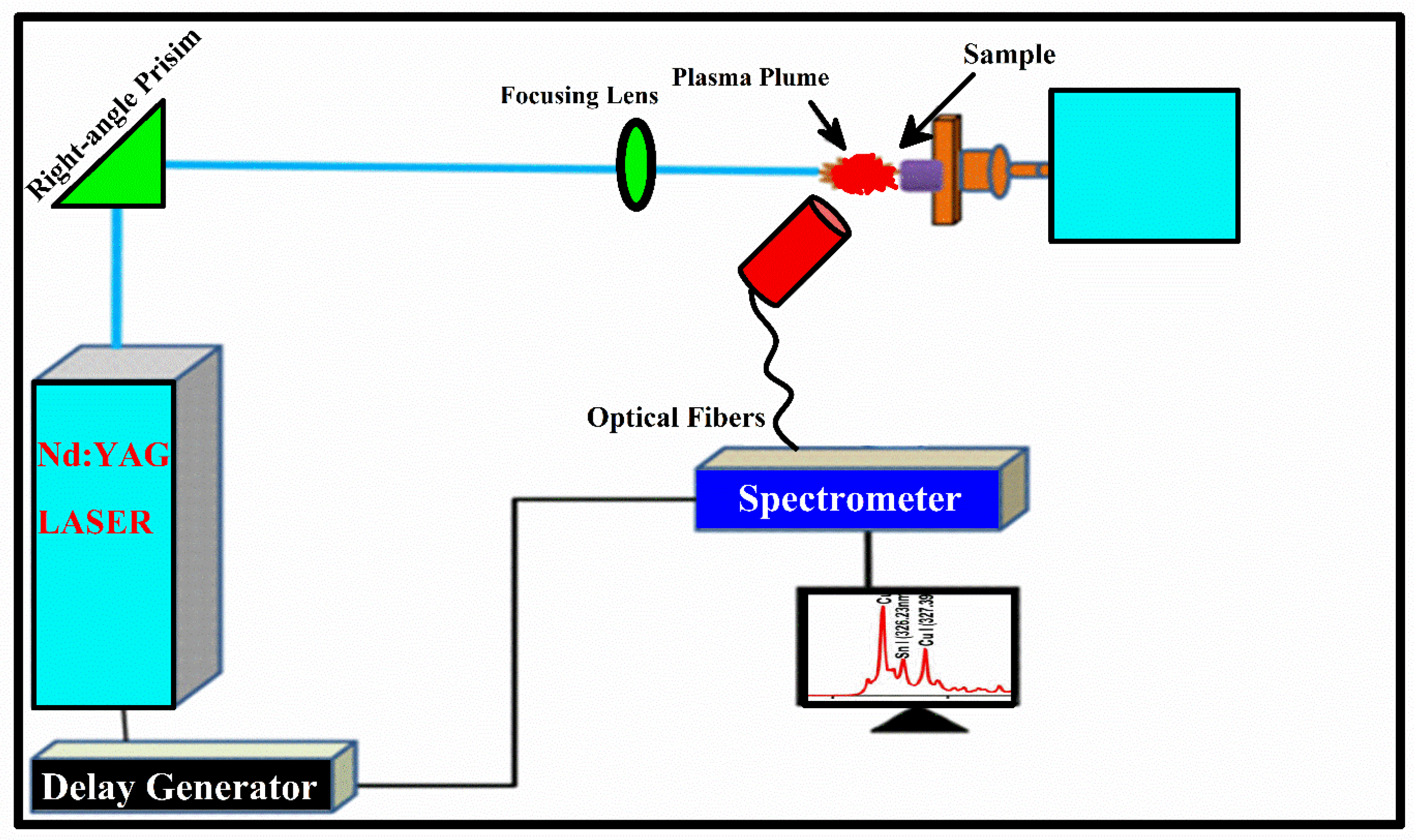
2. Experimental Setup

The schematics of LIBS experimental setup utilized for the analysis of Cu-Fe alloy is illustrated in Figure 1. The same LIBS experimental setup is used as described in our previously reported articles [22,23,24,25]. In short, a pulse of second harmonic (2ω), with pulse duration of 5 ns, 10 Hz pulse repetition frequency, 10 μs integration time, and a 2 μs delay were kept fixed to record emission spectra. The Nd: YAG laser capable of delivering 400 mJ energy at wavelength 1064 nm and 200 mJ energy at wavelength 532 nm was used to induce the plasma. The variation in laser energy was carried out by measuring Q-switch flash lamp (FL-QS) time delay and the amount of energy delivered to the target with the help of an energy meter. The convex lens containing a 20 cm focal length was utilized to direct the laser beam of energy ≈ 80 mJ upon the target surface of the Fe-Cu alloy sample. The sample under investigation was kept on the rotating frame to provide a clean and free-from-deep crevices surface of the target laser for every laser shot. LIBS2000+ detection system (Ocean Optics, Inc.) contains a set of five miniature spectrometers, each with a slit size of 5 μm within the range from 200 nm to 720 nm. The light emitted from optical plasma was recorded by the LIBS2000+ spectrometer detection system using the optical fibers with the collimating lens placed at around 45° to the plasma plume. The dark signal was removed via the OOLIBS2000 software to obtain the actual optical emission signal.

For the comparative elemental study, an ICP-AES analysis of the Cu-Fe alloy sample was also acquired. The plasma is generated at a 1.6 kW power, and Ar gas was also utilized for supplemental cross flows at a 10 L/min flow rate. To perform an ICP-AES analysis, a sample solution was prepared using 70 mg/kg of fine dehydrated powder of the Cu-Fe alloy sample blended with 3 mL laboratory grade (HNO₃) along with 6 mL hydrofluoric acid (HF). The as-prepared solution having a mixture of pure Cu and Fe was heated at around 400 K temperature for one hour in a microwave oven equipped with PTFE pots (CEM, USA) for target sample digestion. Afterward, the solution was collected into a flask and was then used for the ICP-AES chemical analysis using a Thermo-Fisher IRIS Intrepid II ICP-AES system.

3. Results and Discussion

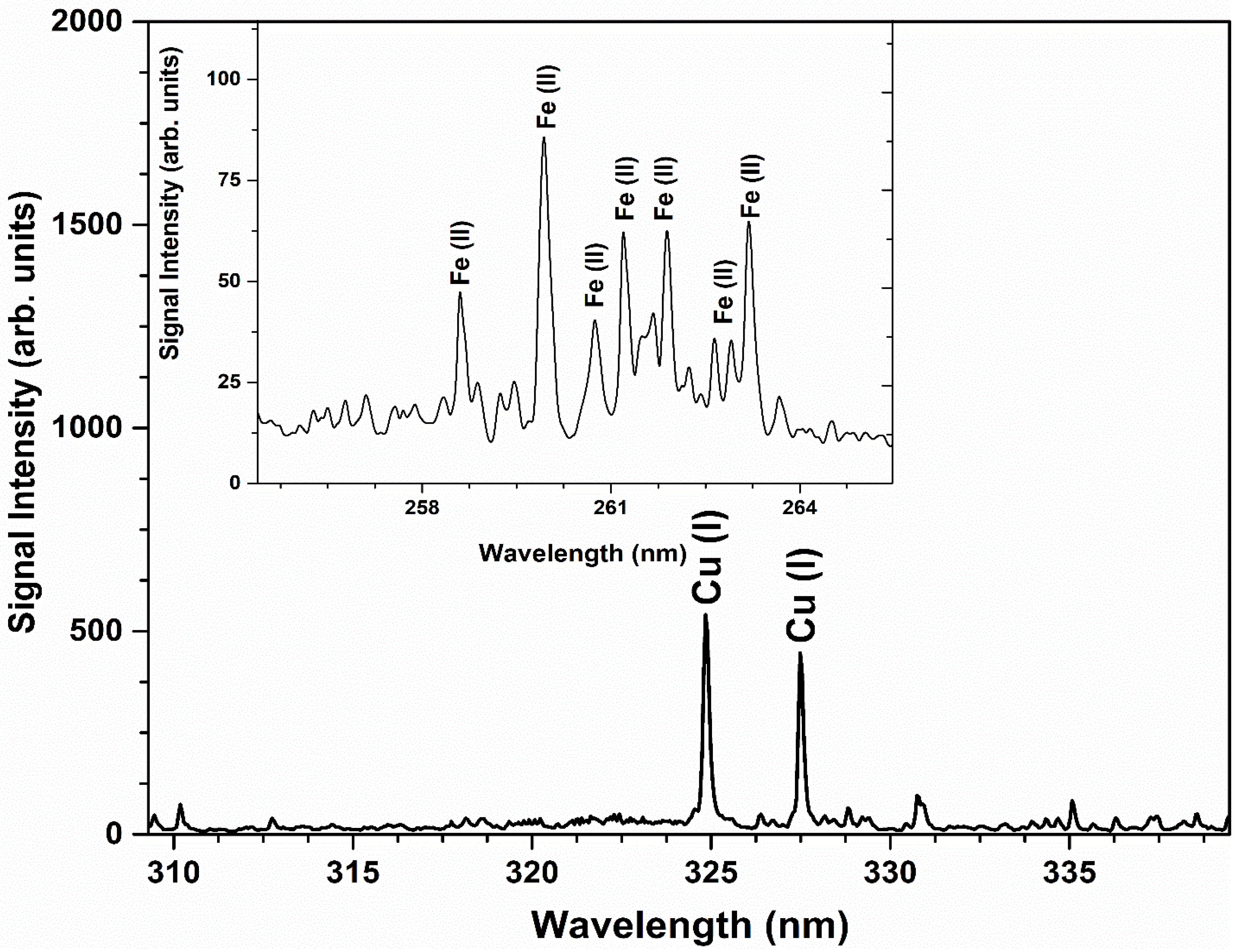
3.1. LIBS Emission Analyses

In Figure 2, we present the emission spectrum of the Fe-Cu alloy sample, which ranges from 323–330 nm and 370–378 nm. This optical wavelength region’s excellent signal-to-noise ratio (SNR) is observed as free from self-absorption and spectral interference. The spectrum shows strong emission lines of Cu I at 324.75 nm and 327.39 nm, along with a bunch of iron emission lines among wavelength regions from 370 nm to 378 nm. The atomic and ionic emission lines of Cu and Fe are recognized by comparing the relative intensity, upper- and lower-level energy, transition probability, and statistical weight, respectively, via the NIST database [26]. To improve the accuracy of LIBS analysis, including plasma characterization, the line selection rules have been considered throughout the qualitative analysis. According to this rule, the following conditions for the selection of lines are designated:

• For the calculation of plasma number density and plasma temperature, ground state transition lines are ignored;
• The transitions corresponding to lower energy below 6000 cm⁻¹ are eliminated to reduce the self-absorption influence on the emission line;
• The transitions having a transition probability lesser than ≈10⁶ s⁻¹ are omitted to avoid the time intrusion between emission time and time related to the plasma variations.

The whole Cu-Fe spectrum from 200 to 720 nm contains different spectral lines of Cu and Fe in the UV-VIS visible region, while the H, N, and O spectral lines are identified in the near-infrared region. The spectrum recorded using OOLIBS2000 software 200 nm to 720 nm wavelength region shows Cu and Fe emission lines are present as dominant in the Fe-Cu alloy plasma. However, H, O, and N spectral lines appeared in the spectrum due to air breakdown. Therefore, only well-resolved emission lines, free from self-absorption and spectral interference, were assumed for the plasma characterization and the CF-LIBS compositional measurement.

Figure 2. Optical emission spectrum as a function of wavelength (nm) using a 10 μs and 2 μs integration time and delay time, respectively between the opening of the window and the laser pulse, showing the expected lines of Cu and Fe in the UV-VIS region.

Figure 2. Optical emission spectrum as a function of wavelength (nm) using a 10 μs and 2 μs integration time and delay time, respectively between the opening of the window and the laser pulse, showing the expected lines of Cu and Fe in the UV-VIS region.

3.2. Local Thermodynamical Equilibrium and Optically Thin Condition

Both parameters of plasma excitation temperature and plasma density are the most basic, prominent, and significant factors in LIBS analytical analysis. Spectral characterization of laser-induced plasma is believable with verification of the OT and LTE conditions. Various methods are used to check the OT condition for LIBS optical plasma. The OT condition for plasma can be verified from the linear trend of Boltzmann plots and by comparing the experimentally observed intensity and theoretically estimated intensity ratio. To check the OT condition, we have compared the experimentally observed intensity and theoretically estimated intensity ratio using the following relation [27]:

$$\frac{{\mathrm{I}}_1}{{\mathrm{I}}_2}=\frac{{\mathrm{A}}_1{\mathrm{g}}_1{\mathsf{\lambda }}_2}{{\mathrm{A}}_2{\mathrm{g}}_2{\mathsf{\lambda }}_1} e^{-\frac{\left({\mathrm{E}}_1-{\mathrm{E}}_2\right)}{{\mathrm{k}}_B\mathrm{T}}}$$

(1)

Here,${ \mathrm{I}}_1$ and ${\mathrm{I}}_2$ are experimentally observed line intensities; A, g, and λ represent the transition probability and statistical weight for upper energy level and wavelength, respectively. Similarly, E and ${\mathrm{k}}_B\mathrm{T}$ is the upper-level energy and plasma excitation temperature (eV). The left-hand side of Equation (1) represents the experimentally observed line intensities ratio, and the other side represents the theoretically calculated values using spectroscopic parameters for the same spectral lines. The spectral wavelength of the emission lines with corresponding spectroscopic parameters is listed in

Table 1. Spectroscopic parameters for neutral iron and copper emission lines along with calculated theoretical and experimental intensities ratios.

Element	λ (nm)	$\mathbf{A}$$\left({\mathbf{s}}^{-1}\right)$	Accuracy	${\mathbf{g}}_{\mathit{k}}$	Intensity (a.u.)	${\mathbf{E}}_{\mathit{k}}\left(\mathbf{eV}\right)$	Experimental Ratio	Theoretical Ratio
Cu l	515.32	6.0 × 107	C+	4	1079	6.19	0.532	0.539
	521.82	7.5 × 107	C+	6	2028
Fe l	372.13	6.7 × 106	B	3	61.5	5.82	0.586	0.536
	382.18	7.3 × 106	B	5	104.9	5.85

. The experimentally observed and theoretically calculated intensity ratios for spectral lines 372.13 nm and 382.18 nm for Fe I are 0.598 and 0.591, while for Cu I lines with wavelength 515.32 nm and 521.82 nm, the intensity ratios are 0.53 and 0.59, respectively. The estimated average plasma temperature (0.69 eV) from Boltzmann plots belonging to Cu I and Fe I spectral lines was used in Equation (1) to validate the OT condition. The OT results were found within 10% relative uncertainty. Thus, the OT condition is validated, which ensures that the LIBS optical plasma is OT. For more clarification, the experimentally measured intensities, spectroscopic parameters, and intensity ratios of the Fe and Cu emission lines are presented in Table 1.

The LTE condition for LIBS optical plasma was checked with two different methods. In the first method, the McWhirter criterion for minimum electron number density was used to verify the LTE condition [27].

$$N_e\left({\mathrm{cm}}^{-3}\right)\ge 1.6\times {10}^{12}\times {\left(T\right)}^{1/2}{\left(∆E\right)}^3$$

(2)

Here, $∆E$ represents the variance among the lower as well as upper energy levels, while T represents the plasma excitation temperature. The calculated electron density from Equation (2) must be smaller than the electron number density estimated from the stark broadened line profile. The plasma number density estimated using the McWhirter criterion was $3.7\times {10}^{14}$ cm⁻³ having Fe I emission line at 407.47 nm, ΔE = 3.04 eV, and T = 0.69 eV. While electron number density using SBM was $2.73\times {10}^{16} {\mathrm{cm}}^{-3}$ for both Fe I and Cu I, the above relation (2) becomes $2.73\times {10}^{16}{ \mathrm{cm}}^{-3}\ge 3.7\times {10}^{14} {\mathrm{cm}}^{-3}$, validating the LTE condition. Similarly, the average electron number density calculated from the Saha–Boltzmann equation was $3.9\times {10}^{16} {\mathrm{cm}}^{-3}$, which is also greater than the plasma density measured from the McWhirter criterion. Therefore, results show that LIBS Cu-Fe alloy plasma is in LTE.

3.3. Plasma Excitation Temperature

We have measured the plasma excitation temperature from the relative spectral intensity of the emission lines of iron and copper using the following Boltzmann equation [28,29,30,31,32]:

$$ln(\frac{I_{ki}{\lambda }_{ki}}{A_{ki}{g}_k})=ln(\frac{N\left(T\right)}{U\left(T\right)})-\frac{E_k}{k_{B}T}$$

(3)

The g_k and E_k are the statistical weight and energy for the upper level, respectively. The $U\left(T\right)$ is the partition function, $k_B$ is the Boltzmann constant, $N\left(T\right)$ denotes the population of excited states, and T represents the plasma temperature of plasma, while $A_{ki}$ and ${\lambda }_{ki}$ represents the transition probability and wavelength, respectively. From Equation (3), upper energy level verses $\mathit{ln}(\frac{I_{ki}{\lambda }_{ki}}{A_{ki}{g}_k})$ shows a linear trend, and the line slope is equal to the 1/$k_B{T}_e$ yields the $T_e$ (plasma temperature).

Various Fe I emission lines correspond to the wavelength at 358.26 nm, 414.60 nm, 418.95 nm, 426.42 nm, 470.74 nm, and 561.52 nm. Cu I lines heaving wavelength at 406.26 nm, 465.11 nm, 521.82 nm, 515.32 nm, 458.69 nm, and 570.02 nm are used to construct Boltzmann plot for the calculation of plasma excitation temperature. The relevant spectroscopic parameters used for the construction of the Boltzmann plot are given in

Table 2. Spectroscopic parameters of neutral iron (Fe I) and copper (Cu I) used to construct Boltzmann plot.

Element	Wavelength λ (nm)	Transition Probability Ak (s−1)	Accuracy	Statistical Weight gk	Upper Energy Level Ek (cm−1)
Fe l	358.26	2.44 × 105	C	7	47,693.2
	414.61	3.78 × 105	C+	11	48,231.3
	418.95	2.70 × 106	D	7	53,661.1
	426.42	1.62 × 106	C+	7	50,611.3
	470.74	2.92 × 105	C	5	44,183.6
	561.52	2.39 × 105	C	5	38,678.0
Cu l	406.26	2.10 × 107	C	6	55,391.3
	458.69	3.20 × 107	C+	6	62,948.3
	465.11	3.80 × 107	C+	8	62,403.3
	515.32	6.00 × 107	C+	4	49,935.2
	521.82	7.50 × 107	C+	6	49,942.0
	570.02	2.40 × 105	C+	4	30,783.7

. The excitation temperature is estimated from the slope of the line after linear fit to the data points, i.e., k_BT. The Boltzmann plots based on the Fe I and Cu I optical spectral lines are shown in Figure 3. The plasma excitation temperatures were calculated as (8068 ± 800) K for Cu I and (7960 ± 800) K for Fe I.

3.4. Electron Number Density

SBM is a reliable and convenient technique for the estimation of plasma number density. The electron number density via the SBM is calculated for optically thin lines, and its value is reliable if the shape of the experimentally measured peak is consistent with a theoretically built profile. The plasma number density is calculated as follows [33,34]:

$$N_e\left({\mathrm{cm}}^{-3}\right)=\left[\frac{FWHM}{2{\omega }_s}\right]\times N_r$$

(4)

where FHWM is the full width at half-maximum (FWHM), stark broadening parameter ${\omega }_s$ was taken from the literature [27] for Cu and Fe atomic emission lines at various temperatures, $N_r$ is the reference number density (${10}^{16}$ cm⁻³ for the neutral species and ${10}^{17}$ cm⁻³ for singly ionized species). The FWHM of the Cu and Fe emission line was calculated using the Voigt fit to the line profile by considering the Stark width (ω_s), 0.06 ± 0.01 nm instrumental width, and 0.005 nm the Doppler width, respectively. The estimated average value of plasma number density from the Stark broadened line profiles of Fe and Cu is $2.73\times {10}^{16} {\mathrm{cm}}^{-3}$. In Figure 4, the dots signify the experimental data, and the red lines show the Voigt fitting.

In the Saha–Boltzmann method, the plasma number density can be calculated using the spectral lines of both the neutral and ionized plasma constituents [35] as follows:

$$n_e\left({\mathrm{cm}}^{-3}\right)=\frac{I_z}{I_{Z+1}}\times 6.04\times {10}^{21}\times \left(T^{\frac{3}{2}}\right)\times e^{\frac{-E_{k,z+1}+E_{k,z}-{\chi }_z}{k_{B}T}}$$

(5)

where $I_z$ represents the intensity of neutral lines, $I_{Z+1}$ is the intensity of ionized lines, $E_{k,z+1}$ is the upper-level energy for singly ionized species, $E_{k,z}$ is the upper-level energy for neutral species, ${\chi }_z$ the ionization energy of neutral species, $k_B$ is the Boltzmann constant in eV, and T denotes the average electron excitation temperature. The average electron number density calculated for iron and copper from the Saha–Boltzmann equation is $3.9\times {10}^{16} {\mathrm{cm}}^{-3}$, which is close to the electron number density calculated from the SBM.

3.5. Calibration Free-LIBS

The CF-LIBS method does not require calibration curves, reference samples, and matrices matched with the known composition of a sample. Different calibration-free methods can be used to find the elemental composition of elements in a sample. We have used the well-known CF-LIBS method in this present study for elemental analysis. For the LTE plasma, the Boltzmann equation is used to find the composition of neutral species in a Cu-Fe alloy sample.

$$F{C}^z=I_k\frac{U^z\left(T\right)}{A_K{g}_K}{e}^{\left(E_k/k_{B}T\right)}$$

(6)

Factor F is an experimental factor that corresponds to the ablated mass, $C^z$ is the concentration of neutral atoms, and $I_k$ is the integrated line intensity. The Saha–Boltzmann equation is utilized to measure the composition of ionized atoms ($C^{z+1})$.

$$C^{z+1}=\left(\frac{C^z }{N_e}\right)\left[\frac{{\left(2m_e{k}_{B}T\right)}^{3/2}}{h^3}\right]\frac{2U_{z+1}}{U_z}\exp \left(\frac{E_{ion}}{k_{B}T}\right)$$

(7)

The total concentration of both the species such as neutral and singly ionized charge particles is calculated as follows:

$$C^T=C^z+C^{z+1}$$

(8)

The weight percentage composition is calculated via the following relation:

$$C^T\left(\%\right)=\left(\frac{C^T\times W^T}{{\sum }_{n=1}^n{C}^T\times W^T}\right)\times 100$$

(9)

3.6. LIBS: Boltzmann Intercept Method

In the Boltzmann Intercept Method, slope intercepts from the Boltzmann plots are estimated individually for each element present in a sample. While the Cu-Fe plasma satisfies the LTE criterion, all the Boltzmann plots will, hence, have a similar slope with different slope intercepts. For assuming an optically thin LTE plasma, by taking the logarithm of both sides of Equation (6), the Boltzmann equation is rewritten as follows:

$$ln\left(\frac{I_k}{A_K{g}_K}\right)=-\frac{E_k}{k_{B}T}+ln\left(\frac{F{C}^z}{U_z\left(T\right)}\right)$$

(10)

Equation (10) shows a linear equation of the structure as ($y=ax+b$) and can be used to draw Boltzmann plots, where ‘$a=-\left(1/k_{B}T\right)$’ represents the slope, and ‘$b=ln\left(F{C}^z/U_z\left(T\right)\right)$’ represents the slope intercept. Equation (10) in terms of slope intercept ‘b’ can be written as follows:

$$C^z=\frac{1}{F}{U}^z\left(T\right)e^b$$

(11)

As slope ‘a’ corresponds to the temperature of the sample plasma, which is almost constant, slope intercept ‘b’ will be unique and relates to the composition of the species. For each species, the total composition of an element is the sum of the composition of both ionized as well as neutral species of that element as $(C^T=C^z+C^{z+1}$). The experimental factor F can be achieved by considering the normalized sum of the concentration of all the species to unity as follows:

$$\sum C^z=\sum \left(\frac{1}{F}{U}^z\left(T\right)e^b\right)=1$$

(12)

The chemical composition wt.% calculated using the CF-LIBS method and the relative standard deviation (RSD) are shown in

Table 3. Relative elemental composition wt.% estimated via the CF-LIBS technique along with RSD.

Elements
Composition wt.% ± RSD Using CF-LIBS
Cu	18.09 ± 1.26
Fe	81.91 ± 5.73

. The results show that the alloy sample contains Cu and Fe as major ingredient elements. To calculate the relative errors in the chemical composition wt.%, we determined the RSD of each element’s composition that appears in the target sample.

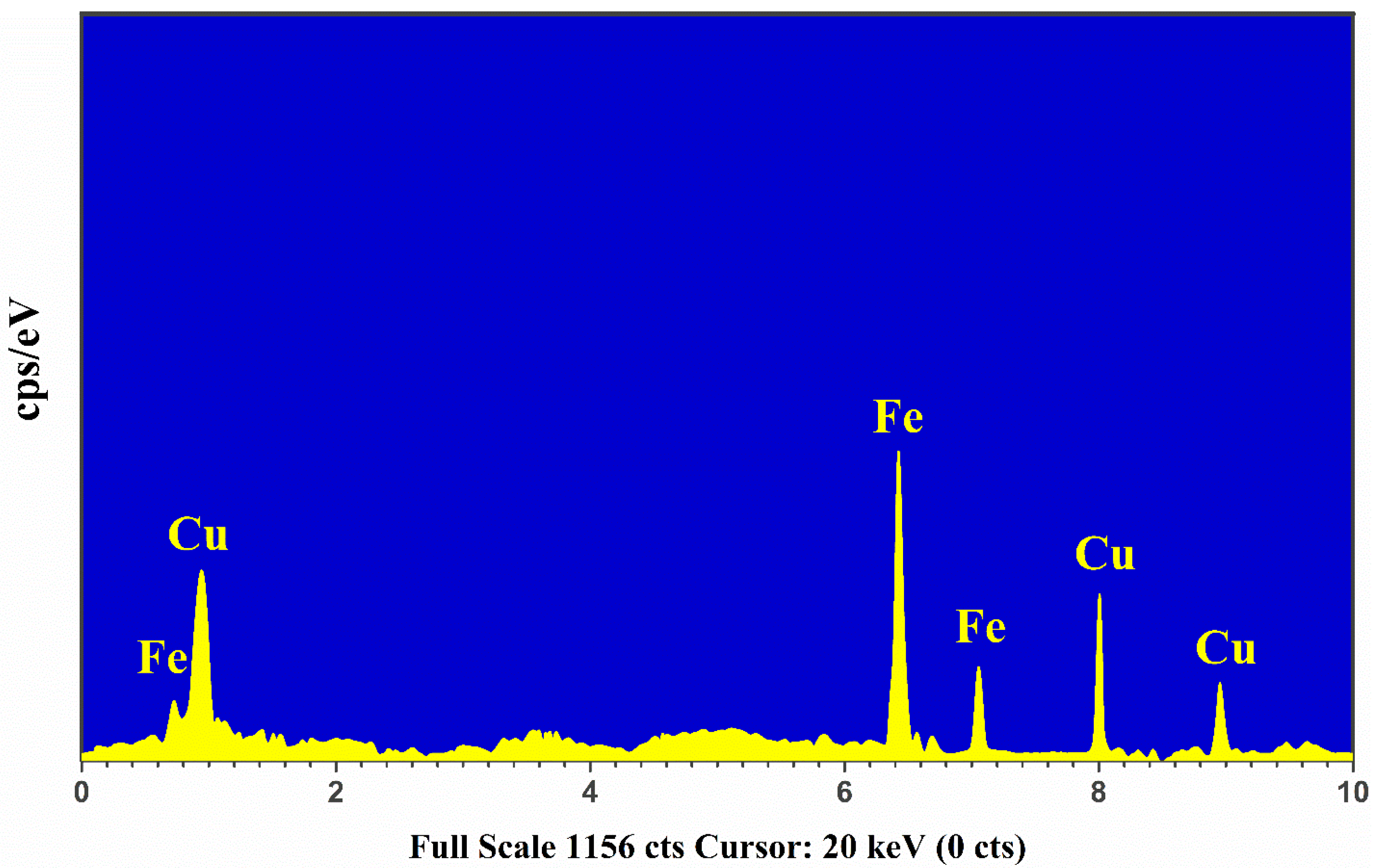
3.7. Energy Dispersive X-ray (EDX) Studies

The Energy Dispersive X-ray (EDX) is a spectroscopical technique used for qualitative and quantitative study based on the characteristic X-ray emissions that determine the elemental signatures in a sample. The EDX chemical analysis is employed in different areas, such as the medical, metal industry, plants, minerals, drugs, and cement industries. In this study, we utilized the EDX spectrum of the Cu-Fe alloy sample that was obtained via the Oxford EDX Instruments (X-MaxN-20) operated at 30 keV having a depth profile of 2 μm.

In Figure 5, we present the characteristic X-ray emission spectrum of the Cu-Fe alloy sample showing the K-shell and L-shell electronic transitions. For the qualitative analysis, the strong Lα₁, Kα₁, and Kβ₁ lines of Cu at 0.929 keV, 8.047 keV, and 8.91 keV, respectively, were detected showing the presence of copper in the target sample. Similarly, the strong characteristic X-ray emission lines correspond to Fe at 0.71 keV, 6.4 keV, and 7.1 keV due to Lα1, Kα₁, and Kβ₁ transitions, respectively, were identified in the spectrum. For quantitative measurement, commercially available software was utilized to integrate the detected X-ray emission lines of Cu and Fe. The EDX estimated composition (%) within the 5% error of Cu and Fe in the sample is presented in Figure 5. The error appears due to the detector’s dead time, and it can be detracted using the EDX software. The relative uncertainty in the EDX quantitative analysis is around ~5% and usually occurs owing to the line integration procedures using the EDX software.

3.8. ICP-AES Analysis

For the qualitative analysis, the ICP-AES spectrum of the Cu-Fe alloy sample comprising signal amplitude versus wavelength is demonstrated in Figure 6. Various emission peaks of singly ionized Fe at 258.58 nm, 259.94 nm, 260.71 nm, 261.19 nm, 261.76 nm, 262.56 nm, 262.83 nm, and 263.13 nm, while strong emission peaks of atomic Cu at 324.75 nm and 327.39 nm were detected in the ICP-AES spectrum. For the quantitative analysis, the weight percent (%) of the detected elements Cu and Fe is shown in

Table 4. Comparative study of Cu-Fe alloy sample composition using different analytical tools.

Elements	CF-LIBS ± RSD	Boltzmann Intercept Method ± RSD	EDX ± RSD	ICP-AES ± RSD	Standard
Cu	18.09 ± 1.26	19.11 ± 0.95	22.21 ± 1.33	21.09 ± 0.84	20
Fe	81.91 ± 5.73	80.89 ± 4.04	77.79 ± 4.66	78.91 ± 3.15	80

.

3.9. Comparative Analyses

In the following, we compared the results obtained using CF-LIBS, Boltzmann Intercept Method, EDX, and ICP-AES with that of the standard components provided by the company, as shown in Table 4. In CF-LIBS, the estimated relative composition of the Fe and Cu in the alloy sample is 81.91% and 18.09%, respectively. Similarly, the calculated composition of Fe and Cu elements using ICP-AES, Boltzmann Intercept Method, and EDX is (78.91% and 21.09%), (80.89% and 19.11%), and (77.79% and 22.21%), respectively. The mean (μ) and standard deviation (σ) of the estimated composition of the elements; Fe and Cu are (79.9 wt.% and 1.45) and (20.1 wt.% and 1.44), respectively. The compositional results from ICP-AES were found very near to the standard within a 2% relative error. For the Cu element, CF-LIBS results were found similar to the ICP-AES and standard values because the variation in signal intensities of Cu emission lines was detected as very analogous in both LIBS and ICP-AES measurements. However, the Fe composition results obtained using CF-LIBS, Boltzmann Intercept Method, and EDX were found quite deviating from the standard values within 5%, 4%, and 5% error, respectively. CF-LIBS uncertainty in the Fe composition appeared due to variation in signal intensities of Fe emission peaks compared to ICP-AES. The results estimated using different techniques show that the Cu-Fe alloy sample has the highest composition of Fe (~80%).

Typically, LIBS analysis is affected by the chemical matrix effect more rigorously than ICP-AES due to the high-density plasma. However, in this analysis, LIBS has detected all the optical emission peaks of Fe and Cu from the wavelength region 200 nm to 720 nm showing good detection limits, but ICP-AES covers only a particular wavelength region from 250 nm to 500 nm showing only two peaks of Cu along with different peaks of Fe. A major constraint of the Boltzmann Intercept Method is the prerequisite to constructing the Boltzmann Plots for all the ingredient elements that exist in the sample, which is quite easy for major elements than traces. In our experiment, both elements Cu and Fe are present as a major ingredient in the alloy sample, so results obtained using the Boltzmann Intercept Method are quite compatible with that of the other analytical techniques and standards. EDX is generally utilized for the qualitative and quantitative measurements of a target sample. The EDX depth profile is usually ~5 μm, its detection minimum value is ~0.1 wt.%, and elements starting from Na to U can be easily identified. The elements which are present in compositions >0.1% can be identified in the EDX spectral analysis. Therefore, in this study, the elements Cu and Fe with compositions >15% are determined very accurately within a 5% error. In addition, to achieve RSD values, the results presented in Table 4 were taken from the different techniques at several measurements using an identical Cu-Fe alloy sample such as seven measurements for CF-LIBS and five measurements for other techniques on the same experimental conditions.

4. Conclusions

In summary, we have investigated the qualitative and quantitative characterization of the Fe-Cu alloy sample using the LIBS spectroscopical technique. For the qualitative analysis, the LIBS spectrum was acquired by focusing a 2nd harmonic (2ω) Q-switched Nd: YAG pulse laser (at a wavelength of 532 nm) on a sample surface. For the CF-LIBS quantitative measurements, sample plasma was considered by calculating the plasma excitation temperature and electron plasma number density having established the LTE and optically thin plasma assumptions. The average value of the plasma excitation temperature (~800 K) and electron plasma number density (~$3.3\times {10}^{16} {\mathrm{cm}}^{-3}$) was used to estimate the composition. For the comparative studies, the same sample was analyzed using EDX and ICP-AES techniques. The results estimated using CF-LIBS were compared with the EDX, and ICP-AES showed excellent agreement with the standard composition (Cu: 20%; Fe: 80%) provided by the manufacturer. Therefore, CF-LIBS has a potential technique for material quantification, and it can be employed in the metal industry for elemental characterization.

References

1. Noll, R.; Fricke-Begemann, C.; Connemann, S.; Meinhardt, C.; Sturm, V. LIBS analyses for industrial applications–an overview of developments from 2014 to 2018. J. Anal. At. Spectrom. 2018, 33, 945–956. [Google Scholar] [CrossRef] [Green Version]
2. Smith, W.F.; Hashemi, J.; Presuel-Moreno, F. Foundations of Materials Science and Engineering; McGraw-Hill: New York, NY, USA, 2006; Volume 509. [Google Scholar]
3. Belmont. Adding Iron into Copper Alloys: Properties and Advantages. Available online: https://www.belmontmetals.com/adding-iron-into-copper-alloys-properties-and-advantages/ (accessed on 6 February 2023).
4. American Society For Testing Materials (Revised Annually). “Copper and Copper Alloys.” Annual Book of ASTM Standards; ASTM International: West Conshohocken, PA, USA, 2004; Volume 2.1. [Google Scholar]
5. Breedis, J.F.; Caron, R.N. “Copper Alloys (Wrought).” Kirk-Othmer Encyclopedia of Chemical Technology, 4th ed.; John Wiley & Sons, Inc.: Hoboken, NJ, USA, 1993; Volume 7, pp. 429–473. [Google Scholar]
6. Babilas, R.; Bajorek, A.; Spilka, M.; Radoń, A.; Łoński, W. Structure and corrosion resistance of Al–Cu–Fe alloys. Prog. Nat. Sci. Mater. Int. 2020, 30, 393–401. [Google Scholar] [CrossRef]
7. Huttunen-Saarivirta, E. Microstructure, fabrication and properties of quasicrystalline Al–Cu–Fe alloys: A review. J. Alloys Compd. 2004, 363, 154–178. [Google Scholar] [CrossRef]
8. Laplanche, G.; Bonneville, J.; Joulain, A.; Gauthier-Brunet, V.; Dubois, S. Mechanical properties of Al–Cu–Fe quasicrystalline and crystalline phases: An analogy. Intermetallics 2014, 50, 54–58. [Google Scholar] [CrossRef]
9. Ciucci, A.; Corsi, M.; Palleschi, V.; Rastelli, S.; Salvetti, A.; Tognoni, E. New procedure for quantitative elemental analysis by laser-induced plasma spectroscopy. Appl. Spectrosc. 1999, 53, 960–964. [Google Scholar] [CrossRef]
10. Griem, H.R. Principles of Plasma Spectroscopy; Cambridge University Press: Cambridge, UK, 1997. [Google Scholar]
11. Cremers, D.A.; Radziemski, L.J. Handbook of Laser-Induced Breakdown Spectroscopy; John Wiley & Sons: Hoboken, NJ, USA, 2013. [Google Scholar]
12. Fichet, P.; Menut, D.; Brennetot, R.; Vors, E.; Rivoallan, A. Analysis by laser-induced breakdown spectroscopy of complex solids, liquids, and powders with an echelle spectrometer. Appl. Opt. 2003, 42, 6029–6035. [Google Scholar] [CrossRef] [Green Version]
13. Iqbal, J.; Alrabdi, T.A.; Fayyaz, A.; Asghar, H.; Shah, S.K.H.; Naeem, M. Elemental study of Devarda’s alloy using calibration free-laser induced breakdown spectroscopy (CF–LIBS). Laser Phys. 2023, 33, 036001. [Google Scholar] [CrossRef]
14. Gomba, J.M.; D’Angelo, C.; Bertuccelli, D.; Bertuccelli, G. Spectroscopic characterization of laser induced breakdown in aluminium–lithium alloy samples for quantitative determination of traces. Spectrochim. Acta Part B At. Spectrosc. 2001, 56, 695–705. [Google Scholar] [CrossRef]
15. Mohamed, W.T.Y. Improved LIBS limit of detection of Be, Mg, Si, Mn, Fe and Cu in aluminum alloy samples using a portable Echelle spectrometer with ICCD camera. Opt. Laser Technol. 2008, 40, 30–38. [Google Scholar] [CrossRef]
16. Goode, S.R.; Morgan, S.L.; Hoskins, R.; Oxsher, A. Identifying alloys by laser-induced breakdown spectroscopy with a time-resolved high resolution echelle spectrometer. Presented at the 2000 Winter Conference on Plasma Spectrochemistry, Fort Lauderdale, FL, USA, January 10–15, 2000. J. Anal. At. Spectrom. 2000, 15, 1133–1138. [Google Scholar] [CrossRef]
17. Ismail, M.A.; Imam, H.; Elhassan, A.; Youniss, W.T.; Harith, M.A. LIBS limit of detection and plasma parameters of some elements in two different metallic matrices. J. Anal. At. Spectrom. 2004, 19, 489–494. [Google Scholar] [CrossRef]
18. Castro, J.P.; Pereira-Filho, E.R. Twelve different types of data normalization for the proposition of classification, univariate and multivariate regression models for the direct analyses of alloys by laser-induced breakdown spectroscopy (LIBS). J. Anal. At. Spectrom. 2016, 31, 2005–2014. [Google Scholar] [CrossRef]
19. Shakeel, H.; Haq, S.U.; Aisha, G.; Nadeem, A. Quantitative analysis of Al-Si alloy using calibration free laser induced breakdown spectroscopy (CF-LIBS). Phys. Plasmas 2017, 24, 063516. [Google Scholar] [CrossRef]
20. Ali, I.; Pan, Y.; Jamil, Y.; Shah, A.A.; Amir, M.; Al Islam, S.; Fazal, Y.; Chen, J.; Shen, Z. Comparison of copper-based Cu-Ni and Cu-Fe nanoparticles synthesized via laser ablation for magnetic hyperthermia and antibacterial applications. Phys. B Condens. Matter 2023, 650, 414503. [Google Scholar] [CrossRef]
21. Ahmed, N.; Shahida, S.; Kiani, S.M.; Razzaq, M.I.; Hameed, M.U.; Iqbal, S.M.Z.; Abbasi, S.A.; Rafique, M.; Baig, M.A. Analysis of an Iron-Copper Alloy by Calibration-Free Laser-Induced Breakdown Spectroscopy (CF-LIBS) and Inductively Coupled Plasma–Mass Spectrometry (ICP-MS). Anal. Lett. 2022, 55, 2239–2250. [Google Scholar] [CrossRef]
22. Alrebdi, T.A.; Fayyaz, A.; Asghar, H.; Elaissi, S.; Maati, L.A.E. Laser Spectroscopic Characterization for the Rapid Detection of Nutrients along with CN Molecular Emission Band in Plant-Biochar. Molecules 2022, 27, 5048. [Google Scholar] [CrossRef]
23. Alrebdi, T.A.; Fayyaz, A.; Ben Gouider Trabelsi, A.; Asghar, H.; Alkallas, F.H.; Alshehri, A.M. Vibrational Emission Study of the CN and C2 in Nylon and ZnO/Nylon Polymer Using Laser-Induced Breakdown Spectroscopy (LIBS). Polymers 2022, 14, 3686. [Google Scholar] [CrossRef]
24. Iqbal, J.; Mahmood, S.; Tufail, I.; Asghar, H.; Ahmed, R.; Baig, M.A. On the use of laser induced breakdown spectroscopy to characterize the naturally existing crystal in Pakistan and its optical emission spectrum. Spectrochim. Acta Part B At. Spectrosc. 2015, 111, 80–86. [Google Scholar] [CrossRef]
25. Fayyaz, A.; Asghar, H.; Alshehri, A.M.; Alrebdi, T.A. LIBS assisted PCA analysis of multiple rare-earth elements (La, Ce, Nd, Sm, and Yb) in phosphorite deposits. Heliyon 2023, 9, e13957. [Google Scholar] [CrossRef]
26. ASD. NIST Atomic Spectra Database Lines Form. Available online: https://physics.nist.gov/PhysRefData/ASD/lines_form.html (accessed on 6 February 2023).
27. Konjević, N.; Lesage, A.; Fuhr, J.R.; Wiese, W.L. Experimental Stark widths and shifts for spectral lines of neutral and ionized atoms (a critical review of selected data for the period 1989 through 2000). J. Phys. Chem. Ref. Data 2002, 31, 819–927. [Google Scholar] [CrossRef]
28. Vassileva, E.; Furuta, N. Application of iminodiacetate chelating resin muromac A-1 in on-line preconcentration and inductively coupled plasma optical emission spectroscopy determination of trace elements in natural waters. Spectrochim. Acta Part B At. Spectrosc. 2003, 58, 1541–1552. [Google Scholar] [CrossRef]
29. Lesage, A.; Lebrun, J.L.; Richou, J. Temperature dependence of Stark parameters for Fe I lines. Astrophys. J. 1990, 360, 737–740. [Google Scholar] [CrossRef]
30. Griem, H.R. Plasma Spectroscopy; McGraw Hill: New York, NY, USA, 1964. [Google Scholar]
31. Miziolek, A.; Palleschi, W.V.; Schechter, I. Laser Induced Breakdown Spectroscopy-Fundamentals198 and Applications; Cambridge University Press: Cambridge, UK, 2006. [Google Scholar]
32. Cremers, D.A.; Radziemski, L. Handbook of Laser Induced Breakdown Spectroscopy; Wiley: New York, NY, USA, 2006. [Google Scholar]
33. Aragon, C.; Aguilera, J.A. Determination of the local electron number density in laser-induced plasmas by Stark-broadened profiles of spectral lines: Comparative results from Hα, Fe I and Si II lines. Spectrochim. Acta Part B At. Spectrosc. 2010, 65, 395–400. [Google Scholar] [CrossRef]
34. Noll, R. Laser-Induced Breakdown Spectroscopy—Fundamentals and Applications; Springer: Berlin/Heidelberg, Germany, 2012. [Google Scholar]
35. Unnikrishnan, V.K.; Alti, K.; Kartha, V.B.; Santhosh, C.; Gupta, G.P.; Suri, B.M. Measurements of plasma temperature and electron density in laser-induced copper plasma by time-resolved spectroscopy of neutral atom and ion emissions. Pramana 2010, 74, 983–993. [Google Scholar] [CrossRef]
Figure 1. LIBS spectroscopy experimental setup used to acquire optical spectrum.
Metals 13 01188 g001
Figure 3. Measured Boltzmann plots for the measurement of plasma temperatures from the Cu I and Fe I emission lines.
Metals 13 01188 g003
Figure 4. Voigt fit (red color) to the line profiles (blue dots) of Fe (I) and Cu (I) lines at 382.18 nm and 510.55 nm, respectively.
Metals 13 01188 g004
Figure 5. The EDX spectrum of Cu-Fe alloy sample.
Metals 13 01188 g005
Figure 6. ICP-AES spectrum of Cu-Fe alloy sample revealing different dominant emission peaks of Cu and Fe.
Metals 13 01188 g006