Abstract
This study introduces a methodology for detecting the location of signal sources within a metal plate using machine learning. In particular, the Back Propagation (BP) neural network is used. This uses the time of arrival of the first wave packets in the signal captured by the sensor to locate their source. Specifically, we divide the aluminum plate into several areas, design eight receiving points for receiving the excitation signal, and determine the location of each sound source. In order to train and test the machine learning network, the aluminum plate model was established using the COMSOL numerical simulation platform and the propagation of five peak waves was simulated. Correspondingly, experimental verification was carried out and a scanning laser Doppler vibrometer (SLDV) was used to build an experimental platform to collect the corresponding wave field information to obtain a data set for machine learning. The results show that the trained BP neural network can classify the sound source region in both environments.
1. Introduction
Plate-like structures are widely utilized in large-scale high-end equipment, such as aircraft fuselage and wings, high-speed rail wagons, and liquid fuel storage tanks. Such structures are directly exposed to the external environment and bear loads and vibrations for a long time, which reduce their structural resistance. In extreme cases, sudden disasters occur. Many studies on Structural Health Monitoring (SHM) of sheet metal structures exist in the literature [1,2,3,4,5]. Several industrial fields use Non-Destructive Testing (NDT) based on ultrasonic guided waves in these studies [6,7,8,9,10].
Lamb waves are caused by sound sources within plate-like structures. Damage detection based on Lamb wave is usually based on physical model, through the analysis and processing of the signal obtained by the sensor, and then uses various methods to identify the damage. Therefore, signal processing of guided waves is critical for establishing structural health monitoring. Tobias [11] proposed a general method for computing two dimensional defect locations from the time of arrival at the sensor for isotropic metal sheets. Based on the guided wave theory to study the propagation characteristics of acoustic signals, He et al. [12] tried to introduce a near-field acoustic emission beamforming method to estimate the position of the sound source by using a small sensor array close to the local area. Focusing on the localization of excitation sources, Kundu et al. [13] exploited an optimization-based methodology for source localization for boards with known material information and applied it to carbon/epoxy composite laminates [14,15]. Nucera et al. [16] identified the impact source on an anisotropic composite plate. Dubuc et al. [17] proposed an inversion algorithm to build the relationship between focal depth and amplitude ratio to characterize crack propagation in plates. Nakatani et al. [18] used a sensor cluster-based beamforming technique to calculate the time difference to locate sound sources in anisotropic panels. Ciampa and Meo [19] combined continuous wavelet transform and local Newton iteration method to realize real-time monitoring of shock source location and wave velocity. The damage identification algorithm based on the physical model theory often needs to use an analytical calculation to invert and estimate the whole process of the guided wavefield propagating in the structure. For the complex boundary conditions of high-end equipment, its damage identification and evaluation effects are limited. Various signal analysis methods can interpret the damage information in the signal from different angles. However, the complexity of the guided wave propagation in the structure and its multi-modal and dispersion characteristics make fast and accurate signal analysis difficult.
Sun et al. [20] proposed a near-field source location algorithm based on a uniform linear array and verified the performance of the proposed method using numerical simulation. Tian et al. [21] used numerical simulations to verify a mixed source localization method using MUSIC and sparse signal reconstruction. Ernst et al. [22] used the finite element method to locate the wave source by back-propagating the waveform captured by the laser Doppler vibrometer. Through a series of numerical simulations, Sikdar et al. [23] proposed an impact source localization strategy based on time difference of arrival calculations to locate the impact regions in composite sandwich structures. Introducing a numerical calculation model can deal with complex boundary problems to a certain extent. Still, it is not easy to achieve an accurate evaluation due to the extensive computing resources and time required for numerical calculation.
The rapid increase in computing power in recent years has brought an abundance of available data, opening up more possibilities for data-driven approaches. To make up for the deficiencies of the above-mentioned damage detection methodologies and meet the intelligent requirements of damage detection, it is necessary to consider combining the physical model with the data model, and establish a novel methodology to process the collected signals to improve detection performance.
A novel method for multi-class classification and uncertainty quantification of impact events on composite panels using Bayesian neural networks (BNN) was proposed by Yu et al. [24]. In their study, diagnostic uncertainty due to variations in impact position, angle, and energy under actual operating conditions was considered. Karmakov et al. [25] used Transformer neural network architecture to improve the speed and robustness of impact detection on composite panels, and compared the detection effect with commonly used convolutional neural networks. Seno et al. proposed a series of data-driven methods for structural health detection in composite structures. They used a new data-driven stochastic Kriging-based method for impact localization and maximum force estimation [26], gaining more information by quantifying the uncertainty of reliably localizing impact locations and estimating severity. They also proposed a new gradient method to evaluate the impact force of composite structures under simulated environmental and operating conditions [27]. For the time-of-arrival extraction problem, they developed a novel artificial neural network (ANN)-based feature extraction method for impact localization in sensing composite structures affected by environmental and operational conditions [28]. The research of the above scholars focuses on reducing the impact of environmental factors on detection accuracy, while considering the quantification of uncertainty and the importance of position and force in the detection algorithm. In contrast to composite plate structures, metal structures will sag but not delaminate when subjected to impact loads, and the fact of sag is easily detected.
Ebrahimkhanlou et al. [29] used deep learning to develop a source localization method applied to plate-like structures with stiffeners and rivets. Ebrahimkhanlou and Salamone [30] also studied a stacked autoencoder-based methodology that relies on only one sensor to locate the source of the sound in the layer structure. Hesser [31] considered three machine-learning architectures to distinguish different sound sources in aluminum panels. The above methods all use convolutional neural networks to transform the damage recognition problem into an image classification problem, and often need to perform wavelet transform on the initial time domain signal to obtain a time-frequency scale map.
This paper employs a data-driven methodology based on BP neural networks for further developing the utilization of machine learning methods in damage recognition, hoping to obtain higher computational efficiency and accuracy. First, the wave field of the five-peak narrow-band modulated sine signal applied to a thin aluminum plate was obtained by establishing a numerical simulation model and a physical experimental platform and then using the time of arrival of the first wave packet in the waveform received by different sensors to train the Back Propagation neural network, set up different test sets to verify the prediction results and test the robustness. This paper aims to find the source of the sound generated inside a thin aluminum plate using eight sensors in both simulated and experimental environments. Although the traditional Time Difference of Arrival (TDOA) localization methods can also achieve this goal, most require prior knowledge of materials. They are computationally complex, rely on analytical models, and cannot be fast and accurate, which is very different from data-driven methodologies combined with computing intelligence.
2. Algorithm Theory of BP Neural Networks and Signal Preprocessing
2.1. The Operation Mechanism of the BP Neural Network
A typical BP neural network consists of three parts: the input layer, the hidden layer, and the output layer. There are nodes in each layer, and weights connect the nodes in adjacent layers. Theoretically, with one hidden layer, the BP neural network can approach any nonlinear function according to the predetermined accuracy requirements [32]. The core idea of the BP neural network algorithm is that the training process is mainly divided into two parts: signal forward propagation and error backpropagation. When the input layer receives the signal, it will pass it to the hidden layer. The hidden layer processes the signal according to the connection weight threshold and activation function and then passes it to the output layer. After the output layer receives the signal, it will compare the result with the actual value. The actual value is compared, and the error is obtained according to the connection weights and thresholds between the layers. Then the error is back-propagated [33], as shown in Figure 1.
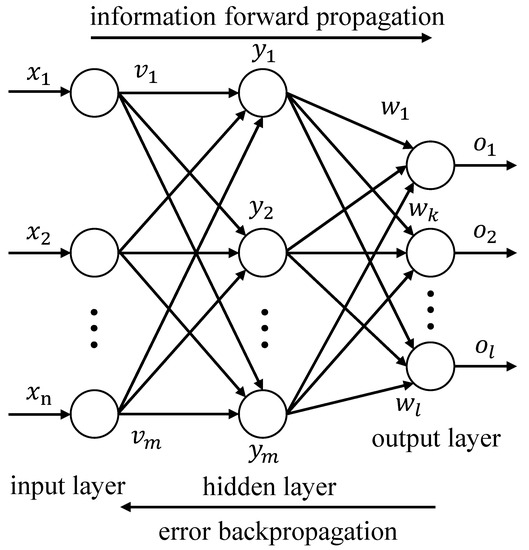
Figure 1.
Schematic diagram of a typical BP neural network.
A standard BP neural network modifies the weights along the reverse of the error-performance function gradient [34]. For the transfer function, if the function is defined and differentiable at a point, the function descends fastest along the reverse of the gradient. Therefore, when using the gradient descent method, the function’s gradient at a certain point should be calculated first. Then the value of the independent variable should be adjusted in a certain step along the opposite direction of the gradient. An output error E is when the network output is not equal to the expected output.
Expanding the above error values to the hidden layer has
Expand further to the input layer
It can be seen from the above formula that the network error is a function of the weights and of each layer, so adjusting the weights can change the error E. The principle of adjusting the weights is to reduce the error continuously, so the adjustment amount of the weights should be proportional to the gradient descent of the error, that is
The negative sign represents gradient descent in the formula, and the constant η ∈ (0, 1) represents the scale coefficient, reflecting the learning rate during training.
The forward propagation process of the signal: the output of the input layer is equal to the input signal of the entire neural network
The input of the i-th neuron in the hidden layer is equal to the weighted sum of Equation (1)
Assuming f(·) is a sigmoid function, the output of the i-th neuron in the hidden layer is
The input of the j-th neuron in the output layer is equal to the weighted sum of
The output of the j-th neuron in the output layer is
The error of the j-th neuron in the output layer is
The total error of the network is
Error signal backpropagation: First, the error backpropagation passes through the output layer, so the weight is adjusted between the hidden layer and the output layer. According to the gradient descent method, the gradient of the error to should be calculated, and then adjusted in a reverse direction
The gradient can be obtained by taking partial derivatives. According to the chain rule of differentiation, we have
Since e(n) is a quadratic function of , its differential is a linear function, so .
Derivative of output layer transfer function
Therefore, the gradient value is
The weight correction is
Introduce the definition of local gradient
Therefore, the weight correction amount can be expressed as
In the output layer, the transfer function is linear, so .
Substitute in and obtain: .
The error signal propagates forward to adjust the weight between the input and hidden layers. Similar to the previous step, there should be , where is the output of the input neuron, and . is the local gradient, defined as
f(g) is the sigmoid function. Since the hidden layer is invisible, the partial derivative of the error cannot be directly solved for the output value of this layer. Here it is necessary to use the local gradient of the output layer node obtained in the previous calculation:
So have
In this paper, the tangent Sigmoid function is used as the activation function in the training of neural networks. The function is continuously differentiable for the input of the range [–1, 1], and the derivative value changes significantly, which can meet the requirements of gradient sensitivity in the process of error backpropagation. Therefore, it is necessary to normalize the sample data before training, and map it to between −1 and 1, to avoid the saturation of neurons in each layer during the training process and, simultaneously, make the model converge more quickly. This paper uses MATLAB software’s mapminmax function to perform the normalization operation. The BP neural network model used subsequently is shown in Figure 2, which is the most typical three-layer structure, including one layer of an input layer, a hidden layer, and an output layer.
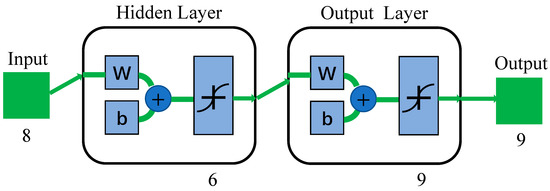
Figure 2.
Schematic diagram of BP neural network structure.
After pre-processing the data, use the MATLAB platform for programming to set the parameters of the BP neural network. The training algorithm chooses the Levenberg-Marquardt algorithm, which is suitable for medium-sized feedforward networks and is one of the fastest. Since the BP algorithm is based on the principle of gradient descent, the learning rate is a critical factor in determining the size of the weight adjustment. If the learning rate is too high, the adjustment amount of each weight will be huge, which will quickly lead to the optimal extreme point in the training process, and the network will not converge. On the other hand, if the learning rate is too low, the adjustment amount of each weight will be too small, and the model will converge slowly. Considering the three-layer BP neural network model chosen in this work, the learning rate is 0.0001, the maximum training times are 50,000, and the minimum error goal is 0.0000001. So far, there is no systematic method for determining the number of hidden layer nodes in the BP neural network. This work uses the empirical formula: the number = of hidden nodes to determine the initial number of hidden nodes, where m is the amount of input neurons, n is the amount of output neurons, and a is a random number between one and 10. Finally, the initial number of hidden nodes is determined to be six, and the increase and decrease methods are utilized to adjust the optimal number of nodes in the subsequent training.
2.2. Processing of the Captured Signals and Data Augmentation
The BP neural network’s training process requires using time-domain signals constructed in the form of vectors or matrices. In this paper, the parameter of the time of arrival of the first wave packet in the time domain signal is selected, and the eight times of arrival obtained from all receivers are collected to construct the input. In the numerical simulation, according to the set integration time step and total duration, the length of each received signal is 1500 samples. It should be pointed out that the low amount of data and lack of variability obtained in a numerical simulation environment is not sufficient to train a neural network. Therefore, it is necessary to enhance the data of the samples to improve the quantity and quality of the samples, thereby improving the model’s generalization ability. Data enhancement is achieved by adding white noise to the initial time-domain signal, and the robustness of the model may also be promoted. As shown in Figure 3, four different white noises are added to the time domain signal: white Gaussian noise, white Uniform noise, white Rayleigh noise, and white Gamma noise. In a wide frequency range, the noise power spectral densities in each band of equal bandwidth are equal, and the amplitudes obey different probability distribution functions. As an example, consider white Gaussian noise to compare the influence of noise with different signal-to-noise ratios on the waveform. As shown in Figure 4, when the signal-to-noise ratio of white Gaussian noise is greater than 35 dB, it has little effect on the time of arrival of the first wave packet, which cannot achieve our purpose of expanding the dataset. While the signal-noise ratio is lowered to 30 dB, the times of arrival start to differ within a specific range. When it is reduced to 25 dB, the white noise severely impacts the initial signal. Moreover, it is hard to distinguish each wave packet. When it is further reduced, to less than 20 dB, it is no longer possible to distinguish between noise and signal. Based on the above comparison, it is proposed to add four kinds of 35 dB white noise to the initial time domain signal for data enhancement.
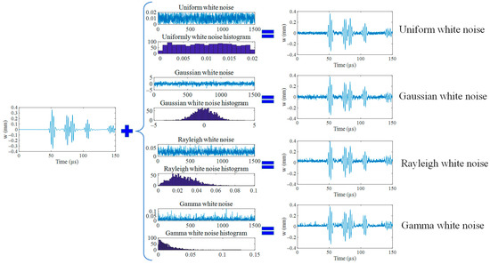
Figure 3.
Adding four different groups of noise for data enhancement.
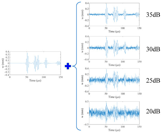
Figure 4.
Effect of Gaussian white noise at different decibels on the initial signal.
Four kinds of white noise are added ten times, respectively into the signal received by each receiving point. Therefore, 40 specimens can be acquired by one operation for each area, and in the nine areas shown in Figure 5, a total of 360 specimens can be obtained. The time of arrival of the first wave packet is extracted for all samples, in this way we can obtain training set data with large variability. We use the time of arrival corresponding to the eight receiving points as the input of the neural network, and the corresponding area number as the output of the model.
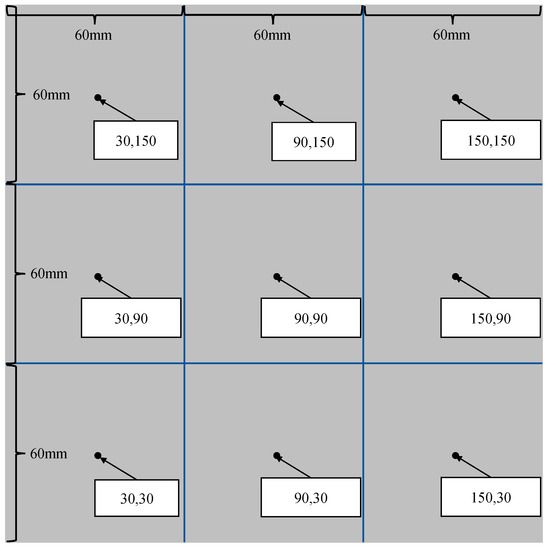
Figure 5.
Schematic diagram of aluminum plate.
3. Establishment of the Finite Element Model
3.1. Choice of Model Arguments
COMSOL numerical software has a powerful multi-physics coupling analysis module, which is suitable for simulating the propagation of ultrasonic-guided waves in plates. A three-dimensional finite element model of the isotropic aluminum plate was established in the solid mechanic’s module. Aluminum has a density of 2700 kg/m3, a Poisson’s ratio of 0.33, and Young’s modulus of 70 GPa. As shown in Figure 5, the size of the aluminum plate model is 180 × 180 × 1 mm, divided into nine areas equally. Each area is a square of 60 mm × 60 mm. The training data actuate point is set at every region’s center, which is (30, 150), (90, 150), (150, 150), (30, 90), (90, 90), (150, 90), (30, 30), (90, 30), (150, 30), corresponding to the coordinates of the central point of region one to region nine in Figure 5.
3.2. Choice of Actuating Loads and Location of Receivers
Because of the multi-mode and dispersion characteristics of Lamb waves in the propagation process, the signal captured by the sensor is very complex. In this paper, to compare and test the robustness of the neural network, five-peak signals with two central frequencies of 200 kHz and 400 kHz are selected, respectively. They are applied to the plate as point loads. Taking 400 kHz as an example, Figure 6 shows the input signal in this model.
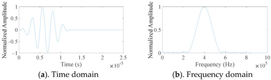
Figure 6.
Excitation Signal Centered at 400 kHz.
In order to enable the model to precisely study the discrepancy in time of arrival of each input signal to the receiving point, eight receivers are set on the surface of the aluminum. As shown in Figure 7, the positions of the eight receiving points are (40, 175), (5, 140), (5, 40), (40, 5), (140, 5), (175, 40), (175, 140), (140, 175).
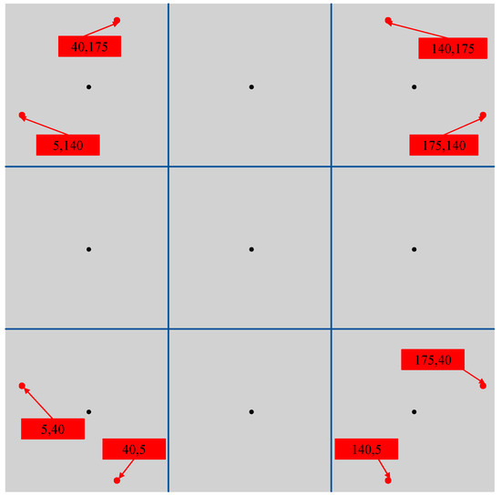
Figure 7.
The location of the receiving point on the surface of the aluminum plate.
3.3. Model Accuracy and Stability
When using the finite element method to simulate Lamb waves, the size of the model grid and the integration time step will have a great impact on the accuracy and stability of the calculation results, so the two need to meet certain conditions. When setting the integration time step, it must be ensured that there are at least 20 times increments in one cycle of the Lamb wave propagating in the plate.
Usually, the mesh size is divided as acceptably as possible under the allowable conditions to upgrade the precision of the simulation outcomes. However, if the mesh is too fine, it will easily affect the computational efficiency. Therefore, it is necessary to consider the simulation model’s calculation accuracy and solution efficiency. The maximum size when meshing should not be larger than one-tenth of the smallest wavelength.
There are mainly two central frequencies of the five-peak signals employed in this study, which are 200 kHz and 400 kHz, respectively. The maximum frequency of the spectrum is 550 kHz, the wavelength corresponding to the S0 mode is 9.6 mm, and the wavelength corresponding to the A0 mode is 3.56 mm. It can be seen from the above that the mesh size should not be greater than 0.356 mm, and the time step should not be more significant than 90.9 ns. Combined with the actual situation, the mesh size in this study is set to 0.35 mm, and the time step is 50 ns.
After setting up according to the above three sections, the Lamb wave propagation process is obtained when the central point of area 3 is excited once as shown in Figure 8. The rest of the regions are excited in the same way. Figure 9 shows the time domain signals captured at the eight receivers at the boundary at this time. It can be observed that there is a significant difference in the time of arrival of the first wave packet due to the different positions of the receiving point from the excitation point. This is precisely the feature that the neural network needs to study in order to map this feature value to its source.
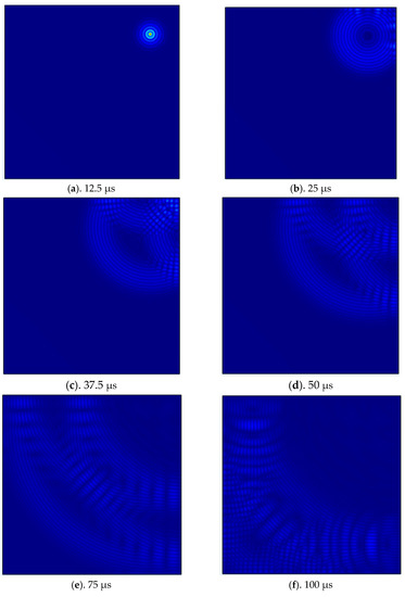
Figure 8.
Wavefield diagrams at different times.
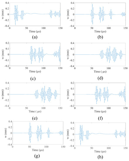
Figure 9.
The initial time domain signals received by the eight receivers after one actuating in the center of area three. (a). The signal received by the receiving point (140, 175). (b). The signal received by the receiving point (40, 175). (c). The signal received by the receiving point (5, 140). (d). The signal received by the receiving point (5, 40). (e). The signal received by the receiving point (40, 5). (f). The signal received by the receiving point (140, 5). (g). The signal received by the receiving point (175, 40). (h). The signal received by the receiving point (175, 140).
4. Analysis of the Location Results of the Five-Peak Narrow-Band Sinusoidal Modulation Signal Actuating Source Area
4.1. Prediction Results When the Excitation Point of the Test Set Is 10 mm Away from the Center of Each Area
After preprocessing the training data set outlined in Section 2.2, arrange multiple sets of different test sets to test whether the trained BP neural network could determine the area to which the new five-peak narrow-band sinusoidal modulation signal excitation source belongs. First, take points near the center point of the area. As shown in Figure 10, the excitation point is set 10 mm from the center of each area, and the same signal with a central frequency of 400 kHz is applied to it for excitation. After the eight receiving points capture the time domain signal, also according to the methodology in Section 2.2, four different white noises are randomly mixed, so that five test samples can be acquired for every excitation. Altogether 45 samples in nine areas are used to test the training effect of the neural network.
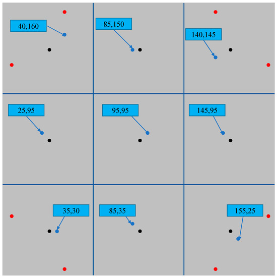
Figure 10.
Test set position slightly off-center.
Having preprocessed the test data, the next step is to input the BP neural network described in Section 2.1 to make predictions. Figure 11 shows the prediction results. All 45 samples were judged correctly, and the trained model accurately predicted the region to which each wave source excitation point belonged at that moment, with a precision rate of 100%. This shows that the BP neural network model constructed in this paper can learn the regularity of the input feature values and map the excitation points to a certain extent near the central point of the training set to their sources.
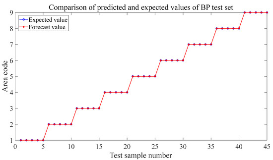
Figure 11.
Prediction results when the excitation point of the test set is within 10 mm of the center.
4.2. Prediction Results When the Excitation Point of the Test Set Is 20 mm Away from the Center of Each Area
In the previous subsection, our model can predict the area where the input source is located with complete accuracy when the location of the test point is near the area’s center point. In this section, we set up another set of test sets, taking points within 20 mm of the area’s center point. As shown in Figure 12, compared to the test set taken in Section 4.1, the points in this test set are closer to the boundaries of adjacent regions. In this case, the signal captured by the receiving point still makes 45 samples as the test set according to the same preprocessing method.
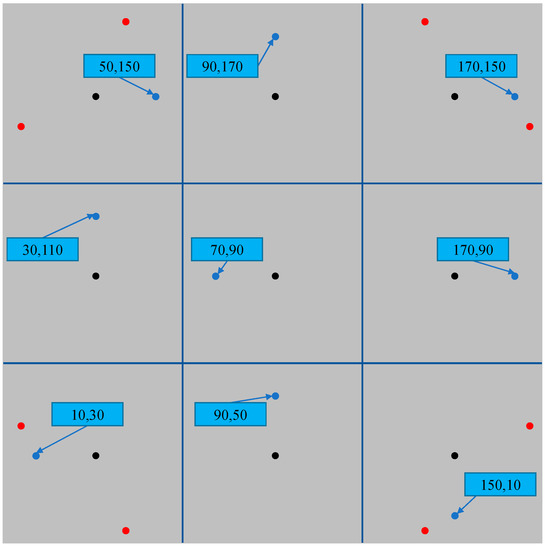
Figure 12.
The test set excitation point is 20 mm away from the center.
Figure 13 shows the prediction results at this time. Although the point of the prediction set is already 20 mm away from the center of the region, which is closer to the border of the adjacent region than the point of the training set, the prediction precision of the model trained with the data set of the center of the region can still reach 100%. It can be seen that the numerical simulation environment can obtain very accurate prediction results, whether near the center or the boundary. This powerfully proves the feasibility of the methodology used in this study. The trained BP neural network could quickly and precisely determine the region where the five-peak narrow-band sinusoidal modulation signal actuating source is located in the aluminum plate.
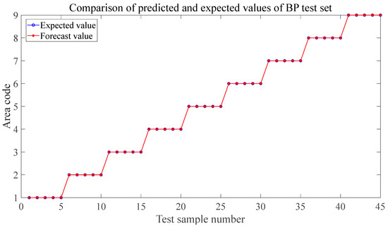
Figure 13.
Prediction results when the excitation point of the test set is within 20 mm of the center.
4.3. The Effect of Different Center Frequencies on the Prediction Results
It can be seen from the above two subsections that the neural network trained in this paper can precisely determine the area where the input source is located, regardless of whether the points in the test set are near the region’s center or the boundary. This section tests the robustness of the neural network by changing the five-peak narrow-band sinusoidal modulation signal input in the simulation. The source in the test set is replaced with a five-peak narrow-band sinusoidal modulation signal with a central frequency of 200 kHz. As shown in Figure 14, the loading position is not changed, and it is still in the center of the region.
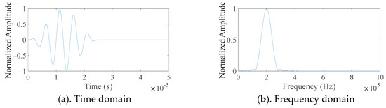
Figure 14.
Excitation Signal Centered at 200 kHz.
Figure 15 shows the prediction results in this situation. When the excitation position is not changed, but only the central frequency of the input signal in the model is changed, the prediction is still accurate. The training set is still the same as before, excited by a 400 kHz five-peak narrow-band sinusoidal modulation signal in the center of every area. The only difference from the test set is that the center frequency is changed to 200 kHz. Next, we changed the data used in the training set to 200 kHz center frequency excitation and set the location of the test point in the same way as Figure 12. At this time, both the training set and the test set used a center frequency of 200 kHz.
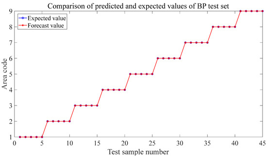
Figure 15.
Predicted results when the center frequency is 200 kHz.
Figure 16 reveals the prediction results in this situation. It can be seen that after changing the central frequency, the model can still judge the position of the source accurately, regardless of whether the location of the test point is changed. This indicates that the neural network in this study is insensitive to the central frequency of excitation and has a certain robustness.
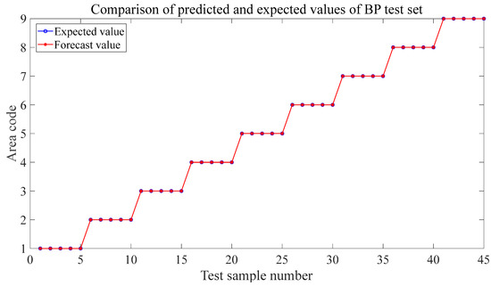
Figure 16.
Prediction results when the center frequency is shifted by 20 mm at 200 kHz.
5. The Result of the Wave Source Localization in the Experiment
5.1. Experiment Layout of Acoustic Source Localization in the Metal Plate Structure
The prediction outcomes in the numerical simulation environment in Section 4 demonstrate that the data-driven methodology proposed in this study could efficiently identify the region where the sound source is located and offers a novel idea for the sound source localization method for isotropic metal sheets. To verify the authenticity of the simulation results, this study used a damage detection platform for sound source localization of aluminum plate structures.
Figure 17 shows the specific arrangement of the experimental platform. First, the preset five-peak narrow-band sinusoidal modulation signal excitation signal is output through the AFG 31000 series signal generator produced by Tektronix, amplified by the Aigtek’s ATA-2021H power amplifier, and then output by the piezoelectric sheet. Secondly, the PSV-500-M Laser Doppler Vibrometer (SLDV) laser head produced by Polytec is used to collect the vibration signal of the corresponding scanning point on the aluminum plate, and the collected time domain signal is sent back to the signal processor. The received signal can be seen through the display. The aim of this study is to detect the position of the sound source in the metal plate, acoustic signals are generated by vibrations, and if there is sound, there must be vibrations. A sound source in the panel generates a transient elastic wave. We want to detect the source of the sound by detecting the vibration.
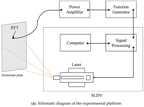
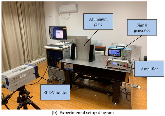
Figure 17.
Experimental platform.
This paper uses an isotropic aluminum plate consistent with the simulation as the experimental object. The size of the aluminum plate is 400 × 500 × 1 mm3. The signal generator is used for excitation and SLDV reception. The position of the scanning point on the surface of the aluminum plate is shown in Figure 18. Eight receiving points should be set up in the same manner as in the simulation, two on each side at a distance of 10 mm from the edge. The sampling time window is set to 400 µs, and the frequency is 5120 kHz, so each received time domain signal has 2048 data points.
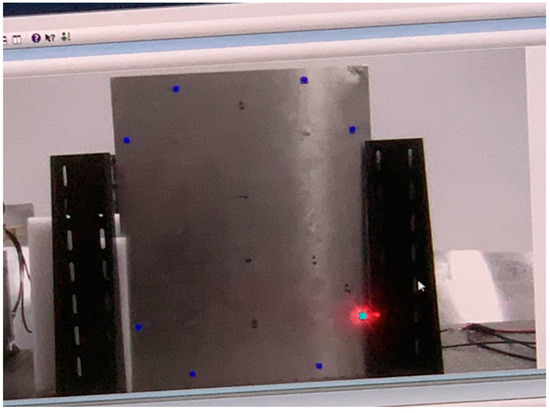
Figure 18.
Scanning Laser Doppler Vibrometer scanning point location.
Figure 19 shows the area division on the back of the aluminum plate, which is divided into nine rectangular regions of 133.3 × 166.7 mm2. Similar to Section 4, two sets of test sets with different locations are also set to check out the model’s forecasting ability. The piezoelectric sheet excites the center point of each area of the aluminum plate with a five-peak narrow-band sinusoidal modulation signal with a central frequency of 200 kHz to obtain the training set data. Both red and blue markers appear in Figure 19, representing two test sets. The distance from the red mark to the center of the region is 30 mm, corresponding to the test set near the center of the region in Section 4.1; the distance from the blue mark to the center of the region is 60 mm, corresponding to the test set near the boundary of the adjacent region in Section 4.2. Set the same 200 kHz five-peak narrow-band sinusoidal modulation signal as when collecting the training set data for periodic excitation.
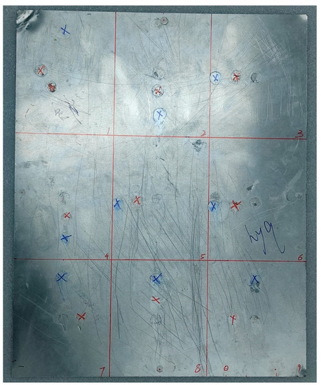
Figure 19.
Area division of aluminum plate.
In Section 2.2, we discuss data augmentation methods for simulated data. However, the received Lamb wave signal is mixed with various environmental noises in a laboratory environment and has a high degree of variability without additional manipulation. Therefore, we omit the step of data augmentation. Figure 20 shows the time domain signals captured by eight receiving points when a five-peak narrow-band sinusoidal modulation signal is an input at the center point of area three. The signals captured by every scanning point are influenced by varying degrees of environmental noise, so we set the signal generator to perform periodic excitation at a particular time interval and collect any ten periodic time domain signals with a fixed time window, and then extract the time of arrival of all the first wave packets to make the neural network input. For the test points, three cycles of the signal were extracted for each region. We obtained 90 samples for training the neural network and 27 samples, each with offsets of 30 mm and 60 mm, as a test set.
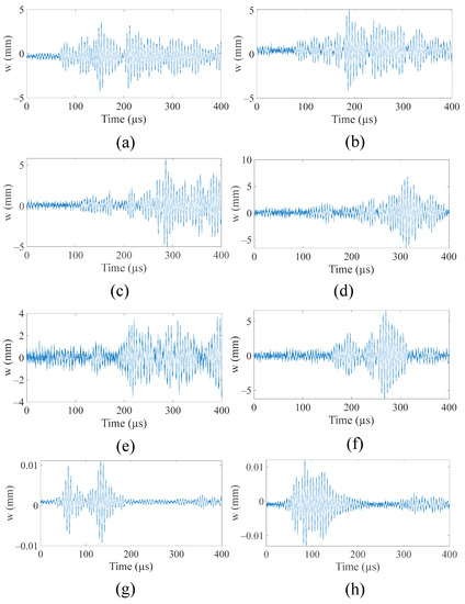
Figure 20.
Signals are obtained at eight scanning points when a five-peak narrow-band sinusoidal modulation signal is input at the center of area 3. (a). The signal received by the receiving point (300, 490). (b). The signal received by the receiving point (390, 400). (c). The signal received by the receiving point (190, 100). (d). The signal received by the receiving point (300, 10). (e). The signal received by the receiving point (100, 10). (f). The signal received by the receiving point (10, 100). (g). The signal received by the receiving point (10, 400). (h). The signal received by the receiving point (100, 490).
5.2. Analysis of the Location Results of the Five-Peak Narrow-Band Sinusoidal Modulation Signal Actuating Source Area in the Experiments
After the same preprocessing, the BP neural network built in Section 2.1 predicts the region where the five-peak narrow-band sinusoidal modulation signal input source is located. After training, the fitting results of the model are shown in Figure 21. It can be seen from the iteration diagram that after the training, the fitting accuracies of training, validation, and testing are: 0.99994, 0.99789, and 0.99812, which are over 0.99 in all cases, which indicates that each dataset fits exceptionally well.
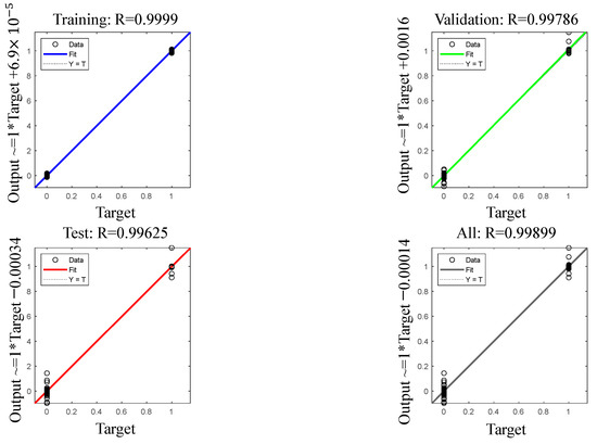
Figure 21.
Regression effect of BP neural network model after training.
Figure 22 and Figure 23 show the prediction results of input sources at different locations. Figure 22 shows that the model reaches the training target after 34 iterations. Figure 23 reveals the forecast results for each of the two test sets. Although the two sets of data are wrongly judged, the accuracy is lower than that in the numerical simulation environment in Section 4. However, for the experiment, this is a satisfactory result. In the case of a test point that is 30 mm away from the center point, that is, near the center point, only one misjudgment occurred in the 27 samples, and the accuracy rate was 96.3%—the situation in the adjacent area. As seen from the blue markings in area three in Figure 19, when offset from the center by 60 mm, the sampling points of the test set in some regions (such as region three) almost coincide with the boundary. Even so, except for the wrong judgment in region three, the other regions can still accurately predict the sound source near the boundary, with a total prediction accuracy of 88.9%. This shows that even in the experimental environment when the environment is greatly disturbed, the trained BP neural network is still capable of making exact judgments of test samples in the area, no matter where the test points are in the area.
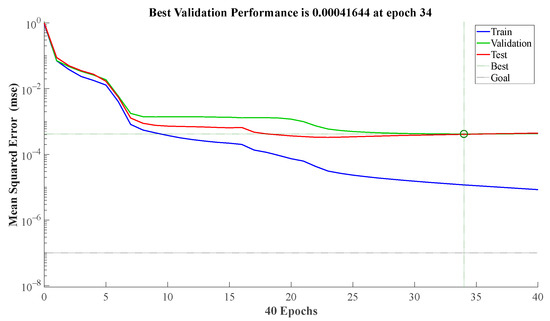
Figure 22.
Graph of the number of network iterations and MSE.
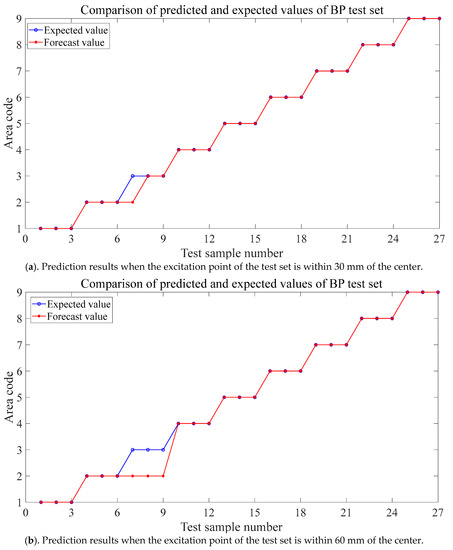
Figure 23.
Prediction results in a laboratory environment.
6. Conclusions
This paper utilizes a machine-learning methodology to localize the source of five-peak narrow-band sinusoidal modulation signals within an isotropic aluminum plate. In order to maximize the time of arrival of the wave packet, two receiving points are set at equal intervals on each edge of the aluminum plate. To prove the feasibility of this methodology, a database is established in two different environments: the COMSOL numerical simulation platform and PZT excitation-SLDV-receiving physical experiment platform. Because the signal obtained by the numerical simulation platform does not have variability, four different groups of noise are added for data enhancement. The prediction results of the BP neural network show that the trained model can map the time of arrival in the signal to the sound source area in both environments. Especially in the numerical simulation environment, the prediction accuracy is excellent. Whether it is near the center of the region or the border of the region, it can reach 100%. All 180 test points can accurately locate the sound source’s area. In the experiments, consequently, environmental factors play a significant role and accuracy is slightly reduced. It can reach 96.3% near the regional center, and 26 of the 27 test points are correctly predicted. When the boundary is reduced to 88.9%, 24 of the 27 test points are correctly predicted. It is still possible to locate the sound source region.
Author Contributions
Conceptualization, investigation, data curation, writing- original draft preparation, Y.H.; software, data curation, validation, methodology, C.T.; conceptualization, methodology, writing- reviewing and editing, W.H. and G.Z. All authors have read and agreed to the published version of the manuscript.
Funding
The authors are grateful for the financial support provided by the National Natural Science Foundation of China (Grant No. 11872025) and the Six Talent Peaks Project in Jiangsu Province (Grant No. 2019-KTHY-059).
Data Availability Statement
No new data were created or analyzed in this study. Data sharing is not applicable to this article.
Conflicts of Interest
The authors declare no conflict of interest.
References
- Shao, Y.; Zeng, L.; Lin, J. Damage detection of thick plates using trailing pulses at large frequency-thickness products. Appl. Acoust. 2021, 174, 107767. [Google Scholar] [CrossRef]
- Cuadrado, M.; Pernas-Sáncheza, J.; Artero-Guerreroa, J.A.; Varas, D. Detection of barely visible multi-impact damage on carbon/epoxy composite plates using frequency response function correlation analysis. Measurement 2022, 196, 111194. [Google Scholar] [CrossRef]
- Hu, M.; He, J.; Zhou, C.; Shu, Z.; Yang, W. Surface damage detection of steel plate with different depths based on Lamb wave. Measurement 2022, 187, 110364. [Google Scholar] [CrossRef]
- Shi, B.; Cao, M.; Wang, Z.; Ostachowicz, W. A directional continuous wavelet transform of mode shape for line-type damage detection in plate-type structures. Mech. Syst. Signal Process. 2022, 167, 108510. [Google Scholar] [CrossRef]
- Nicolas, M.J.; Sullivan, R.W.; Richards, W.L. Large Scale Applications Using FBG Sensors: Determination of In-Flight Loads and Shape of a Composite Aircraft Wing. Aerospace 2016, 3, 18. [Google Scholar] [CrossRef]
- Nazeer, N.; Ratassepp, M.; Fan, Z. Damage detection in bent plates using shear horizontal guided waves. Ultrasonics 2017, 75, 155–163. [Google Scholar] [CrossRef]
- Cui, L.; Zhao, Y.; Zhao, P.; Sun, J.; Jia, Z. Review of noncontact ultrasonic nondestructive testing for the solid materials. Appl. Mech. Mater. 2014, 528, 346–352. [Google Scholar] [CrossRef]
- Zima, B. Determination of stepped plate thickness distribution using guided waves and compressed sensing approach. Measurement 2022, 196, 111221. [Google Scholar] [CrossRef]
- Cho, H.; Hasanian, M.; Shan, S.; Lissenden, C.J. Nonlinear guided wave technique for localized damage detection in plates with surface-bonded sensors to receive Lamb waves generated by shear-horizontal wave mixing. NDT E Int. 2019, 102, 35–46. [Google Scholar] [CrossRef]
- Mahajan, H.; Banerjee, H. A machine learning framework for guided wave-based damage detection of rail head using surface-bonded piezo-electric wafer transducers. Mach. Learn Appl. 2022, 7, 100216. [Google Scholar] [CrossRef]
- Tobias, A. Acoustic-emission source location in two dimensions by an array of three sensors. Non-Destr. Test. 1976, 9, 9–12. [Google Scholar] [CrossRef]
- He, T.; Pan, Q.; Liu, Y.; Liu, X.; Hu, D. Near-field beamforming analysis for acoustic emission source localization. Ultrasonics 2012, 52, 587–592. [Google Scholar] [CrossRef] [PubMed]
- Kundu, T.; Das, S.; Jata, K.T. Point of impact prediction in isotropic and anisotropic plates from the acoustic emission data. J. Acoust. Soc. Am. 2007, 122, 2057. [Google Scholar] [CrossRef] [PubMed]
- Kundu, T.; Yang, X.; Nakatani, H.; Takeda, N. A two-step hybrid technique for accurately localizing acoustic source in anisotropic structures without knowing their material properties. Ultrasonics 2015, 56, 271–278. [Google Scholar] [CrossRef]
- Sen, N.; Kundu, T. A new wave front shape-based approach for acoustic source localization in an anisotropic plate without knowing its material properties. Ultrasonics 2018, 87, 20–32. [Google Scholar] [CrossRef]
- Nucera, C.; White, S.; Chen, Z.M.; Kim, H.; di Scalea, F.L. Impact monitoring in stiffened composite aerospace panels by wave propagation. Struct. Health Monit. 2015, 14, 547–557. [Google Scholar] [CrossRef]
- Dubuc, B.; Ebrahimkhanlou, A.; Livadiotis, S.; Salamone, S. Inversion algorithm for Lamb-wave-based depth characterization of acoustic emission sources in plate-like structures. Ultrasonics 2019, 99, 105975. [Google Scholar] [CrossRef] [PubMed]
- Nakatani, H.; Kundu, T.; Takeda, N. Improving accuracy of acoustic source localization in anisotropic plates. Ultrasonics 2014, 54, 1776–1788. [Google Scholar] [CrossRef]
- Ciampa, F.; Meo, M. Acoustic emission source localization and velocity determination of the fundamental mode A0using wavelet analysis and a Newton-based optimization technique. Smart Mater. Struct. 2010, 19, 045027. [Google Scholar] [CrossRef]
- Sun, J.; Hao, C.; Zheng, Z. Passive Localization of Near-Field Sources Based on Overlapped Subarrays. Circuits Syst. Signal Process. 2020, 39, 502–512. [Google Scholar] [CrossRef]
- Tian, Y.; Sun, X. Passive localization of mixed sources jointly using MUSIC and sparse signal reconstruction. Int. J. Electron. Commun. 2014, 68, 534–539. [Google Scholar] [CrossRef]
- Ernst, R.; Zwimpfer, F.; Dual, J. One sensor acoustic emission localization in plates. Ultrasonics 2016, 64, 139–150. [Google Scholar] [CrossRef] [PubMed]
- Sikdar, S.; Mirgal, P.; Banerjee, S. Low-velocity impact source localization in a composite sandwich structure using a broadband piezoelectric sensor network. Compos. Struct. 2022, 291, 115619. [Google Scholar] [CrossRef]
- Yu, H.; Seno, A.H.; Khodaei, Z.S.; Aliabadi, M.H.F. Structural health monitoring impact classification method based on Bayesian neural network. Polymers 2022, 14, 3947. [Google Scholar] [CrossRef] [PubMed]
- Karmakov, S.; Aliabadi, M.H.F. Deep learning approach to impact classification in sensorized panels using Self-Attention. Sensors 2022, 22, 4370. [Google Scholar] [CrossRef] [PubMed]
- Seno, A.H.; Aliabadi, M.H.F. Uncertainty quantification for impact location and force estimation in composite structures. Struct. Health Monit. 2022, 21, 1061–1075. [Google Scholar] [CrossRef]
- Seno, A.H.; Aliabadi, M.H.F. A novel method for impact force estimation in composite plates under simulated environmental and operational conditions. Smart Mater. Struct. 2020, 29, 115029. [Google Scholar] [CrossRef]
- Seno, A.H.; Khodaei, Z.S.; Aliabadi, M.H.F. Passive sensing method for impact localisation in composite plates under simulated environmental and operational conditions. Mech. Syst. Signal Process. 2019, 129, 20–36. [Google Scholar] [CrossRef]
- Ebrahimkhanlou, A.; Dubuc, B.; Salamone, S. A generalizable deep learning framework for localizing and characterizing acoustic emission sources in riveted metallic panels. Mech. Syst. Signal Process. 2019, 130, 248–272. [Google Scholar] [CrossRef]
- Ebrahimkhanlou, A.; Salamone, S. Single-Sensor Acoustic Emission Source Localization in Plate-Like Structures Using Deep Learning. Aerospace 2018, 5, 50. [Google Scholar] [CrossRef]
- Hesser, D.F.; Mostafavi, S.; Kocur, G.K.; Markert, B. Identification of acoustic emission sources for structural health monitoring applications based on convolutional neural networks and deep transfer learning. Neurocomputing 2021, 453, 1–12. [Google Scholar] [CrossRef]
- Zhang, L.; Wang, F.; Xu, B.; Chi, W.; Wang, Q.; Sun, T. Prediction of stock prices based on LM-BP neural network and the estimation of overfitting point by RDCI. Neural. Comput. Appl. 2018, 30, 1425–1444. [Google Scholar] [CrossRef]
- Lian-Suo, W.; Hua, L.; Di, W.; Yuan, G. Clock synchronization error compensation algorithm based on BP neural network model. Acta Phys. Sin. 2021, 70, 114203. [Google Scholar]
- Song, S.; Xiong, X.; Wu, X.; Xue, Z. Modeling the SOFC by BP neural network algorithm. Int. J. Hydro. Energy 2021, 46, 20065–20077. [Google Scholar] [CrossRef]


Disclaimer/Publisher’s Note: The statements, opinions and data contained in all publications are solely those of the individual author(s) and contributor(s) and not of MDPI and/or the editor(s). MDPI and/or the editor(s) disclaim responsibility for any injury to people or property resulting from any ideas, methods, instructions or products referred to in the content. |
© 2023 by the authors. Licensee MDPI, Basel, Switzerland. This article is an open access article distributed under the terms and conditions of the Creative Commons Attribution (CC BY) license (https://creativecommons.org/licenses/by/4.0/).