Article

Corrosion Behaviour Modelling Using Artificial Neural Networks: A Case Study in Biogas Environment

by
María Jesús Jiménez-Come
*,
Francisco Javier González Gallero
,
Pascual Álvarez Gómez
and
Jesús Daniel Mena Baladés
Escuela Técnica Superior de Ingeniería de Algeciras, Universidad de Cádiz, 11202 Algeciras, Spain
*
Author to whom correspondence should be addressed.
Metals 2023, 13(11), 1811; https://doi.org/10.3390/met13111811
Submission received: 29 September 2023 / Revised: 22 October 2023 / Accepted: 24 October 2023 / Published: 27 October 2023
(This article belongs to the Special Issue Advances in Corrosion and Protection of Materials (Second Edition))

Abstract

:
The main objective established in this work was to develop a model based on artificial neural networks (ANNs) to predict the corrosion status of stainless steel involved in biogas production, analyzing the influence of the material composition and the breakdown potential value. To achieve this objective, an ANN model capable of predicting the corrosion status of the material without the need to perform microscopic analysis on the material surface was proposed. The applicability of the corrosion models was verified via the experimental data considering different factors such as stainless steel composition, biogas environments simulated by artificial solution, temperature, surface finish, and the breakdown potential of the passive layer of stainless steel obtained from electrochemical tests. The optimal prediction performance shown by the model in terms of specificity and sensitivity values were 0.969 and 0.971, respectively, obtaining an accuracy of 0.966. Furthermore, analyzing the influence of the breakdown potential on corrosion modelling, an alternative model was presented capable of predicting the corrosion status automatically, without the need to resort to electrochemical tests for new conditions. The results demonstrated the utility of this technique to be considered in design and maintenance planning tasks for stainless steel structures subjected to localized corrosion in biogas production.

1. Introduction

In recent decades, the increasing energy requirements, in addition to the need to face the consequences of climate change, have encouraged looking for alternative renewable energy sources [1]. The International Energy Agency has estimated that global energy demand will increase by two to three times in this century. With the aim to reduce global warming, in addition to transforming pollutant waste into a valuable resource, the production of bioenergy has become a viable alternative to obtain more cost-effective and less polluting economic activity. It is estimated that the global bioenergy demand will increase by 20% in 2050 [2]. This bioenergy is represented mostly by biogas, bioethanol, and bioelectricity. Biogas is considered a versatile renewable energy source that can replace fossil fuels in power and heat production. It is obtained via anaerobic digestion of organic wastes, offering significant advantages over other types of bioenergy. The use of biodigesters to produce and store biogas via anaerobic digestion can be considered an environmentally friendly technology [3]. Biodigesters are tanks used for energy and biogas production. Raw biogas consists of 60–65% of methane, 30–35% of carbon dioxide, and small percentages of water vapour, H2, H2S, and other impurities [4]. The presence of hydrogen sulphide and other impurities in the production process may cause corrosion, leading to the deterioration of appliances and engines involved in biogas production [5].
Corrosion is considered one of the most critical issues in industrial processes [6]. It can be defined as the degradation of metal or alloy in contact with the environment, reducing its durability. For most applications, it is possible to select materials that show excellent corrosion resistance; however, their costs are often prohibitive. In practice, it is usual to select materials that corrode slowly under uniform corrosion. Nevertheless, a significant proportion of corrosion failures occur due to localized corrosion, which results in failure in a much shorter time. The increasing price of energy encourages the development of cost-effective design solutions for biogas production. In this context, although concrete has been a widely used material in the manufacture of biodigesters, the reduction or even the elimination of corrosion in these tanks is difficult even when special coating is applied. In order to solve these disadvantages, stainless steel has become a suitable option for this application due to its great corrosion resistance, among other factors [7,8].
The high corrosion resistance of stainless steel is explained by the formation of the passive film on the material surface that protects it from aggressive environments. Chromium is the principal element in the composition of stainless steel responsible for the formation of the passive layer. Moreover, other alloying elements may appear in the chemical composition of the alloy, primarily nickel or molybdenum, improving the resistant behaviour of the material. According to the chemical composition, different grades of stainless steel can be obtained with different mechanical, physical, and chemical properties. The chemical composition of the alloy and its surface finish are factors that may have an influence on the corrosion behaviour of the material depending on the environmental conditions [9].
Over the past 50 years, different corrosion studies have concluded that corrosion costs can be estimated to be 3–4% of each nation’s gross domestic product (GDP) [10]. These estimated costs do not consider individual safety or environmental consequences such as incidents, accidents, or outages, among others. Several industries have exposed that via adequate corrosion management, significant cost savings can be achieved [11]. In this context, electrochemical techniques have become a widely used tool in the study of corrosion behaviour [12]. The application of polarization techniques, both potentiostatic and dynamic methods, has been very successful in studying the phenomena involved in the corrosion process. However, in order to understand the behaviour of materials in different environmental conditions, a large number of experimental tests must be carried out. Moreover, the application of electrochemical methods to study the corrosion behaviour of material may influence the corrosion reaction of the samples, and they may not be capable of identifying localized corrosion accurately since these tests often require microscopic analysis of the material surface [13]. This can be tedious and lead to possible undesirable errors, including subjectivity in the experimental results. In order to solve these drawbacks and to improve precision, save time in the evaluation, and eliminate human error, the use of artificial intelligence-based models has been proposed by many researchers. In recent years, the adoption of machine learning in modelling real engineering problems was built on its ability to understand the interrelationships between real input and output data. The potential of these techniques to predict material properties has been reported in scientific literature [14,15,16,17,18,19]. Among the different techniques proposed in the literature, Artificial Neural Networks (ANNs) have become a promising tool that offers great computational power even when a small experimental dataset is considered [20]. In the literature, different models based on ANNs have been presented to model corrosion behaviour.
Pintos et al. [21] developed an ANN model to model atmospheric corrosion processes of carbon steel. The proposed model was compared against a classical regression model to predict the corrosion rate of this material. Diaz et al. [22] proposed an ANN model for the prediction of corrosion damage under different climatological and pollution conditions. The number of neurons in the input layer was defined according to the number of meteorological variables considered in the experimental procedure, whereas the output layer had one unit corresponding to the cumulated penetration. The authors concluded that the presented methodology based on ANNs was an efficient tool for corrosion process modelling from experimental data. These authors continued their studies in [23], where they presented an ANN-based methodology to predict corrosion damage of atmospheric corrosion problems for carbon steel expressed in terms of corrosion penetration. The authors used the model to analyze the relevance of meteorological and pollution factors on corrosion behaviour. Silva et al. [24] applied an ANN to analyze the corrosion defects in pipelines with the aim of finding out the influence of the geometry of the defects on the pipe pressure capacity. Kenny et al. [25] developed an ANN model to analyze the factors that influence the atmospheric corrosion of carbon steel, copper, and aluminum. The authors considered the following as inputs for modelling the meteorological data in addition to local pollution: temperature, solar radiation, relative humidity, precipitation, time of exposure, time of wetness, wind velocity, chloride ions, sulphur compounds, and dustfall. According to the results, the authors concluded that the proposed ANN model could be considered as a good corrosion estimator to predict corrosion rates of the materials. Halama et al. [26] designed a model based on ANN for the assessment of atmospheric corrosion of carbon steel under local geographical conditions, considering climatic conditions (temperature and relative humidity) in addition to pollutant concentrations and precipitation. In that work, the objective was to construct an ANN model that operates with numerous time-dependent parameters predicting related corrosion mass losses accurately. Lin et al. [27] employed the ANN model to predict atmospheric corrosion rates of carbon steel subjected to general and coastal industrial zones. The model was used to determine the most significant factors in corrosion behaviour for the different environments. Tran et al. [28] proposed an ANN model to model atmospheric corrosion in tropical climate conditions. Different meteorological and chemical factors were considered as inputs for modelling, whereas the output provided by the model was related to the atmospheric corrosion rate of carbon steel. Kim et al. [29] used an ANN model to examine the oxidation resistance of Ni-based superalloys, analyzing the effect of the elements to define the optimum composition of the alloy. Zhu et al. [30] presented an ANN model to study the corrosion of carbon steel in reinforced concrete. The authors considered different physical and chemical parameters, including pH, corrosion potential, breakdown potential, and temperature, in addition to cement composition, concrete porosity, and water/cement ratio. They demonstrated the utility of the proposed model to evaluate the corrosion behaviour of materials. Wang et al. [31] presented a model based on ANN as a novel non-destructive testing method of corrosion. According to the electrochemical laboratory tests, the authors predicted the corrosion current density of the gas pipeline accurately. Li et al. [32] proposed an ANN corrosion model to predict the corrosion rate of Q345R steel, considering different factors as input variables: MDEA concentration, total amine concentration, pH, conductivity, and solution type, whereas the target value was defined as the corrosion rate. Soomro et al. [33] applied an ANN to predict the integrity of damaged oil and gas pipelines, considering temperature, pH, pressure, and velocity as input characteristics, whereas Li et al. [34] proposed an ANN for quantitative modelling of corrosion degradation prediction of offshore oil pipelines.
Although there are numerous applications in which neural network-based techniques have been successfully implemented in energy fields [35,36,37], no studies focused on localized corrosion modelling of stainless steel in biogas environments have been found in the literature. This work presents the application of the ANN model to predict the corrosion status of different grades of stainless steel in biogas environments. The proposed model was also applied to analyze the influence of different factors that may affect the corrosion behaviour of stainless steel subjected to these environments. The validity of the model was evaluated with the experimental data set obtained from electrochemical tests in addition to the microscopic analysis of the tested sample. In the experimental procedure, the polarization curves were carried out to assess the localized corrosion resistance of different stainless steel grades, namely pitting [38,39] and crevice [40] corrosion since they are the most important corrosion forms in biogas production [41,42].
In this study, the use of the ANN model allows us to determine the corrosion state of the sample under different conditions simulating biogas environments. Based on our experience in corrosion modelling [43,44], different ANN model configurations were proposed to achieve the established objectives:
Objective 1—To develop an ANN model capable of predicting the corrosion state of stainless steel involved in biogas production without the need for microscopic analysis of the analyzed sample after electrochemical tests.
In this case, three configurations were developed:
MODEL 1: In this case, the ANN model was presented to predict the pitting corrosion status of stainless steel considering data related to the properties of the material (stainless steel composition and surface finish), data obtained from the electrochemical test (breakdown potential of the passive layer) and those data related to the environment to which the material may be exposed in biogas production (temperature and the type of artificial solution). All these data were considered as inputs for the ANN model, while the output was defined by the pitting corrosion status of the sample: 1 for the patterns that suffer pitting corrosion under the conditions analyzed in each case and 0 for those patterns that resist the attack.
MODEL 2: In this case, the model was presented to predict crevice corrosion status. Similar to the previous model, the input variables were defined by the properties of the material (stainless steel composition and surface finish), data obtained from the electrochemical test (breakdown potential of the passive layer) and data related to the environment to which the material may be exposed in biogas production (temperature and the type of artificial solution). However, the output in this case corresponded to the state of crevice corrosion of the sample under study: 1 for the patterns that suffer crevice corrosion and 0 otherwise.
MODEL 3: It was presented as a global model to predict the pitting or crevice corrosion state of the material. In this case, the experimental data used in Model 1, in addition to the data used to develop Model 2, were considered. An additional input variable related to the type of corrosion to be evaluated was included, namely pitting or crevice corrosion. In this way, the input data presented to the model for each pattern were defined by the composition of the stainless steel, surface finish, breakdown potential value obtained from electrochemical tests, temperature, and type of artificial solution, in addition to the type of corrosion that was intended to be predicted (pitting or crevice corrosion). For this model, the output was defined by the corrosion status of the sample under study: 1 for samples that suffered corrosion and 0 otherwise.
The advantage of the proposed models to achieve Objective 1 is that all the models were developed to predict the corrosion status of the stainless steel involved in biogas production without the need to perform microscopic analysis of the material surface after electrochemical tests. This fact avoids adding subjectivity to the results since the optical analysis of the surface depends on the experience of the analyst and may be confusing.
Objective 2—To analyze the effect of PREN (Pitting Resistance Equivalent Number) as an input for corrosion behaviour modelling instead of considering the concentration of the alloying elements in the material.
In this case, MODEL 4, the composition of the material expressed as a percentage of the alloying elements that took part in the composition of the material was replaced by PREN, reducing the number of inputs that were considered in the ANN model.
Objective 3—To analyze the influence of the breakdown potential value obtained from electrochemical techniques in the corrosion modelling of stainless steel in biogas production.
In this case, a new configuration for the ANN model was proposed: MODEL 5. This configuration allowed predicting the corrosion status of stainless steel automatically, without the need to resort to electrochemical tests or microscopic analysis of stainless steel. This can be considered a great advantage in terms of cost savings since it allows knowing, in advance, the corrosion resistance of the material for new environmental conditions related to biogas production automatically.

2. Materials and Methods

With the aim to evaluate the susceptibility of different grades of stainless steel to suffer localized corrosion in biogas production, electrochemical tests were carried out in two different solutions simulating biogas environments. The composition of the different stainless steel grades analyzed is collected in Table 1.
The polarization curves for each sample in different environmental conditions simulating biogas environments were obtained according to ASTM standards: “Convention applicable to electrochemical measurements in corrosion testing” and “Making potentiostatic and potentiodynamic anodic polarization measurements” [45]. The electrochemical tests were carried out in a flat cell for both the pitting and the crevice corrosion analysis, where the temperature was controlled at a constant value by a thermostatic bath (Figure 1b). The test equipment consisted of a potentiostat (EG&G PARC model 263) connected to a computer with the software “Power suite 2.58”. The solution was stirred during the test to homogenize its composition. Two different temperatures were analyzed: 35 °C representing the mesophilic conditions and 50 °C corresponding to thermophilic ones. With the aim to ensure reproducibility in the experimental results, each condition was tested three times. The composition of each artificial solution (AS), representing the biogas environment, is collected in Table 2.
During the experimental procedure, to obtain a comparative assessment of the corrosion resistance of the different grades of stainless steel, the breakdown potential was evaluated for each condition according to the polarization curve obtained from the electrochemical test of each sample according to the environmental conditions. This potential is defined as the potential at which current density suffers an abrupt increase (Figure 1c). Many authors determine this potential as the value of potential corresponding to 100 µA/cm2 at the polarization curve [46]. After the electrochemical test, each sample was analyzed under a microscope to confirm whether it had suffered a localized corrosion attack, see Figure 1d. Therefore, each sample was defined according to the experimental conditions tested: types of artificial solution, temperature, chemical composition of the alloy, surface finish, breakdown potential, and finally, the localized corrosion status. In this way, the experimental database was obtained considering the most relevant factors involved in biogas production that may have an influence on stainless steel durability. This data set was used to develop ANN models to predict the corrosion behaviour of the different grades of stainless steel when they are exposed to the environmental conditions involved in the biogas production process.

2.1. Methodology

Artificial Neural Networks are considered a powerful machine learning technique for modelling real problems, including function approximation and classification problems that cannot be described with traditional mathematical models [47].
The fundamental unit in the ANN architecture is called a neuron or node that mimics the properties of biological neurons. Although there are many different types of ANNs, all of them consist of a set of neurons connected between them. Each unit receives inputs and produces the output based on a mathematical operation. In this case, the input entering the unit is weighted, and a bias is added to its value after passing through the activation function. A structural model is shown in Figure 2.
The structural type of the ANN model proposed in this study was the multilayer feedforward network, see Figure 3. This structure consists of multiple layers of neurons where each neuron in the first layer receives the input while the neurons in the last layer provide the output. The layer between the input and the output is referred to as the hidden layer. All neurons in the input layer are connected to all neurons in the hidden layer, and so on to the output layer.
ANNs technique uses a perceptron to classify a set of patterns of different classes that are linearly separable in the input space. However, the classification fails when non-separable data are presented to the model. In order to solve this drawback, a backpropagation algorithm is introduced [48]. It consists of a supervised learning method that considers the desired output value to train the model. This algorithm is used for backward propagation errors in feed-forward networks. According to the evaluated error, the weights of the network are updated. The algorithm can be considered as a recursive process that continues until a satisfactory performance is achieved.
For ANN models, a critical step is to find the optimal structure since there is no systematic method to determine it. The network incorporated in this study used a two-layer feed-forward network with one hidden layer, as depicted in Figure 3. The number of units in the input layer was specified by the number of parameters considered in each case, as shown in the results section, whereas the number of units in the output layer was specified according to the different corrosion statuses: 1 for corrosion samples and 0, otherwise. Moreover, the selection of the optimal number of hidden layers was made, knowing that those models with one hidden layer can solve most of the non-linear functions in real problems [49].
The optimal ANN structure is defined according to the number of neurons in each hidden layer, the number of hidden layers, the activation function, the learning algorithm and training parameters. Related to the activation functions, they were selected according to the type of layer: the activation function applied in the hidden layer of the multilayer network presented in this study was the sigmoid transfer function since it is the most commonly used function for this layer, whereas the linear transfer function is generally employed in the final layer of a multilayer network with backpropagation. For the learning stage, the Levenberg–Marquardt training algorithm, based on the minimization of the sum of square error, was applied [50]. This algorithm was introduced by Levenberg in 1944 and then rediscovered by Marquardt. It was applied to train the model due to its speed to converge as well as its stability.
For the training stage, the input and output values were normalized to fall in a certain range to increase the convergence ability of the network, improving the training process of the ANN model. Training a neural network that can generalize well to new data is a challenging problem. One of the problems to avoid in the training stage is overfitting. Overfitting occurs when the model classifies those patterns that are presented in the training set correctly. However, the network fails when patterns that have not been used for training are presented to the model.
One method for avoiding overfitting is an early learning-stopping mechanism. In this case, the original data is divided into three subsets: the training set, the validation set, and the test set. The training set is used to adjust the parameters of the network. Out of the patterns that make up the training set, 25% of the data is not used for training and is set aside to form the validation set. This set is used to provide an unbiased evaluation of a model fit tuning model hyperparameters. The validation test determines when overfitting occurs. Finally, the test dataset is used to provide the generalization of the model. In this work, with the aim to avoid overfitting, the experimental data set was divided randomly into three subsets according to the 5-fold cross-validation method for the training stage. The model was trained on the training set and evaluated on the validation set to determine when overfitting occurs. This step is repeated until the optimal values for the ANN model are found. Once the optimal configuration is defined, the classification performance of the model is measured based on the test set, the independent set that has not been presented to the network before. The test set was applied to assess the behaviour of the model to predict the corrosion status of stainless steel. This process was implemented in MATLAB®, 2021. It was repeated 20 times with the different configurations proposed for the ANN model to determine the optimal number of neurons in the hidden layer since too few units in the hidden layer may result in underfitting, whereas too many hidden neurons may lead to overfitting, consuming more time for training the model. The steps for the design of the ANN models are represented in Figure 4.

2.2. Classification Performance of ANN Models

Confusion matrix has been commonly used to evaluate the classification performance of the classification models. In this case, the accuracy of the model is measured based on the comparison between the target value and the output provided by the model. For a classifier and a pattern considered, there are four possible outcomes: true positive, true negative, false positive, and false negative. True positive is a correct classification result (the number of corrosion patterns that have been classified correctly by the model). A false positive is an incorrect result; this means those original no-corrosion patterns have been incorrectly classified by the model as corrosion patterns. The possible outcomes of a classification model are collected in the confusion matrix shown in Table 3.
According to the confusion matrix, the classification performance of the model can be evaluated according to the following equations:
P r e c i s i o n = T P R = T P T P + F P
A c c u r a c y = T P + T N T P + F P + T N + F N
According to Lemeshow and Hosmer [51], the classification models can be divided into the following four categories based on accuracy results:
-
Fail classifier: 0.5 ≤ Accuracy < 0.6;
-
Poor Classifier: 0.6 ≤ Accuracy < 0.7;
-
Fair Classifier: 0.7 ≤ Accuracy < 0.8;
-
Good Classifier: 0.8 ≤ Accuracy < 0.9;
-
Excellent Classifier: 0.9 ≤ Accuracy ≤ 1.0.

3. Results and Discussion

In the study, the main objective was to develop ANN models capable of predicting the corrosion state of different stainless steel grades in biogas environments since localized corrosion can be considered one of the most critical problems in the maintenance of biodigestors used in biogas production. This work focused on pitting and crevice corrosion modelling since they are the two types of localized corrosion that can cause more dangerous damage to the material, affecting its durability. In this section, the results obtained for the different cases proposed in this work are shown in addition to the influence analysis of the parameters considered in the experimental procedure on corrosion modelling.

3.1. Localized Corrosion Behaviour Modelling: Results from OBJECTIVE 1

Three different ANN models were developed to predict the corrosion status of stainless steel used in biogas production. The most relevant characteristics of each ANN model proposed are shown in Table 4. In this case, Model 1 was developed for pitting corrosion modelling; Model 2 was presented to model crevice corrosion behaviour; and Model 3 was proposed to model both corrosion types.
For each case, the number of neurons in the input layer was determined by the number of factors considered in the experimental procedure, whereas the number of neurons in the output layer was defined as a function of the corrosion state: 1 for corrosion patterns and 0 for no-corrosion patterns. For all the models, different numbers of hidden neurons were considered to determine their optimal configurations, from 1 to 15 hidden neurons.
For all cases, the key challenge was to define the optimal structure for the ANN models proposed. In this study, the backpropagation algorithm was applied. The classification performance was validated by comparing the real corrosion status of the original samples with the predictive status provided by the model. As it was indicated previously, the performance of the models was tested by using 5-fold cross validation. This process was repeated 20 times.
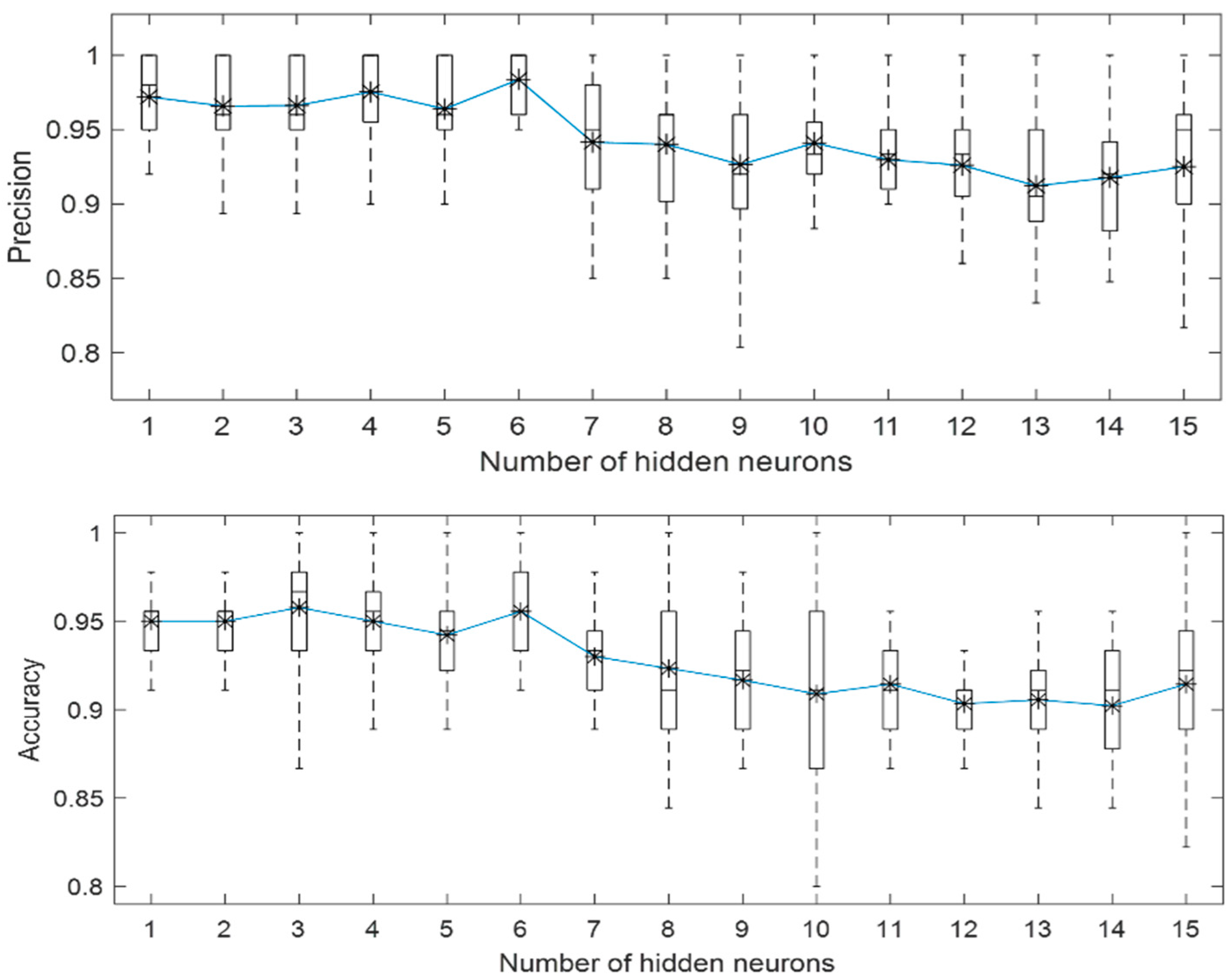
The classification performance of Model 1 proposed to predict the pitting corrosion status of stainless steel in a biogas environment is collected in Figure 5 in terms of precision and accuracy.
According to Figure 5, it is observed that the maximum precision value reached by MODEL 1 to predict the pitting corrosion status of stainless steel in a biogas environment was 0.984 using six neurons in the hidden layer. In terms of accuracy, the maximum value reached by Model 1 was 0.958 with three hidden neurons. As can be seen in Figure 5, as the number of hidden units increased, the model showed a worse performance for both indices: precision and accuracy.
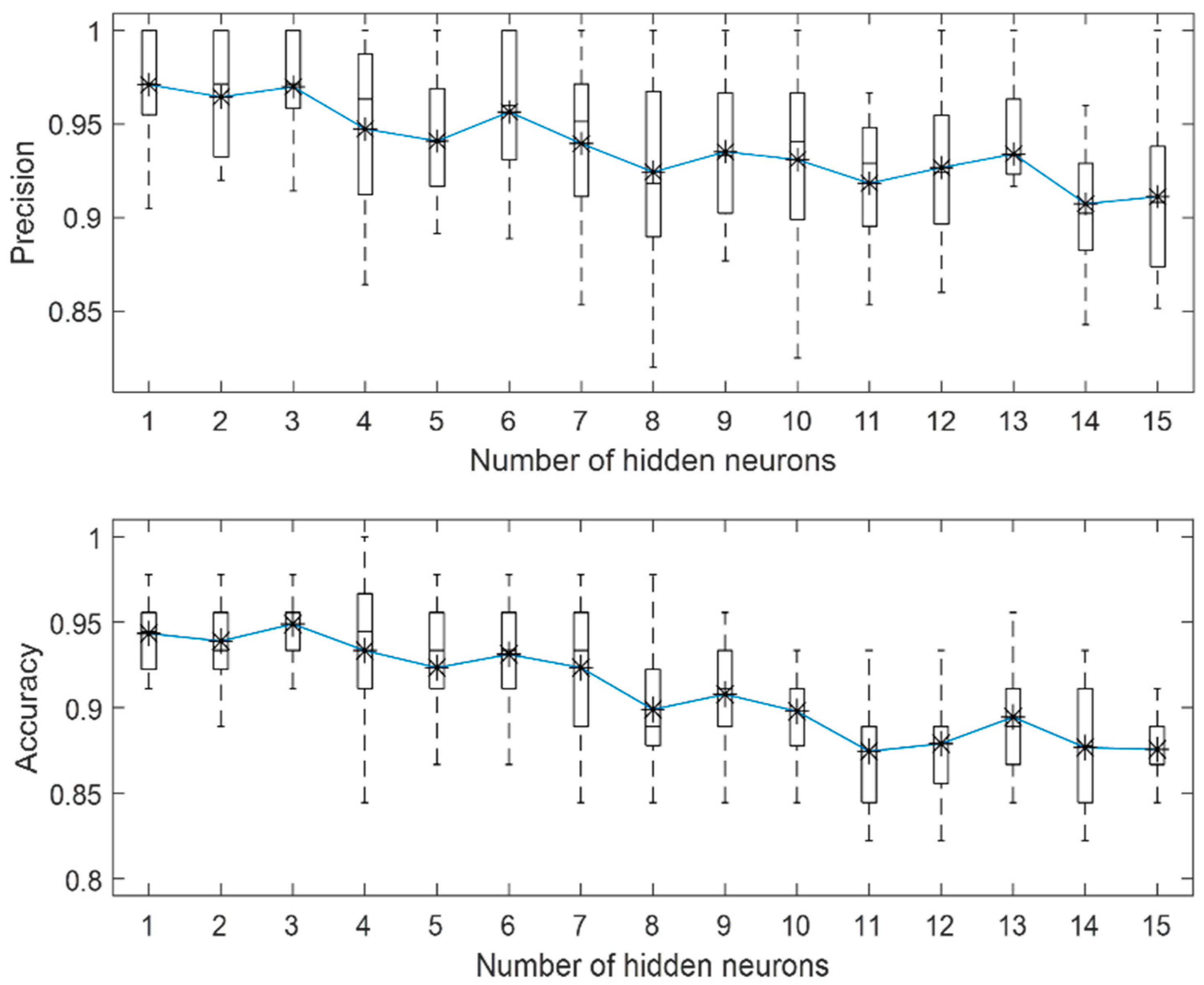
Similar behaviour was obtained for Model 2, which proposed to predict the crevice corrosion status of stainless steel. In this case, the results are shown in Figure 6. According to the figure, the maximum values reached in terms of precision and accuracy were 0.971 and 0.949, respectively. In this case, the optimal structure of the ANN model was obtained by considering three neurons in the hidden layer.
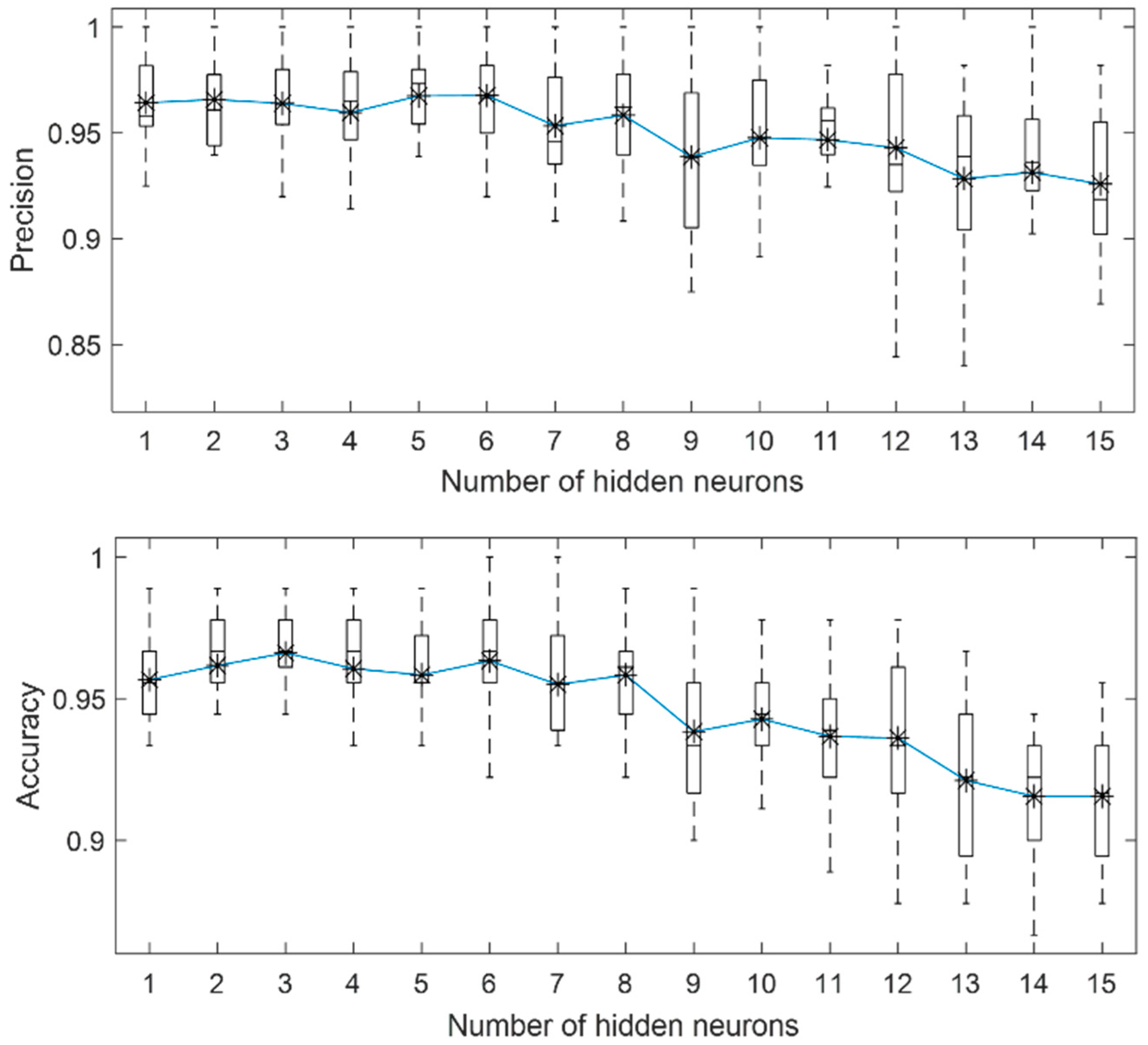
According to the results collected in Figure 5 and Figure 6, the proposed models can be used effectively to determine the corrosion status of both types of attack: pitting (Model 1) and crevice corrosion (Model 2). In this case, the behaviour is similar for both proposed cases, and the capability to predict the corrosion status in terms of precision and accuracy reached maximum values of 0.97 and 0.95, respectively. However, in order to develop a model with greater predictive capacity, a new scenario is proposed (Model 3). In this case, both types of localized corrosion are considered together in the same data set. As shown in Table 4, when Model 3 was proposed, a new input variable was included in the ANN model compared with the previous models. This new input corresponded to the type of corrosion analyzed for each pattern: pitting or crevice corrosion. The results obtained for this model are shown in Figure 7. As shown in the figure, the maximum precision and accuracy values obtained for Model 3 are 0.968 and 0.966, respectively. It is observed that, as in the previous cases, an increase in the number of hidden neurons led to a worse classification performance.
In order to compare the prediction performance for each model (Model 1, Model 2 and Model 3) and to determine the optimal configuration for the proposed models, it is useful to resort to the ROC (receiver operator characteristic) space [52]. In this graphic, the performance of different classification models can be compared. An ROC space is a two-dimensional graph in which the true positive rate (TPR) is plotted against the false positive rate (FPR) for each model. In the ROC space, the better configurations are those located in the upper left corner since these points represent models with high true positive rates and low false positive rates.
Given a model, TPR is the proportion of positive patterns correctly classified by the model over the total number of positive patterns, whereas FPR represents the proportion of incorrectly classified negative patterns over the total number of negative patterns, as shown in the following equations:
T P R = T P T P + F N
F P R = 1   T N T N + F P
According to Figure 8, it is observed that the different configurations proposed for Model 1 stood out for their specificity values, while for Model 2, its different configurations with different numbers of hidden units stood out for its sensitivity values. Furthermore, according to Figure 8, Model 3 showed the best classification performance. This model, considering both types of localized corrosion, outperformed single models: Model 1 and Model 2. In this case, for Model 3, the optimal configuration was obtained when three hidden units were considered in the ANN structure since this is the configuration that is located closest to the upper left corner of ROC space. In this case, specificity values (1 − FPR) of 0.969, sensitivity (TPR) of 0.971 and accuracy of 0.966 are obtained. Based on these values and according to Lemeshow and Hosmer, Model 3 can be defined as an excellent classifier since the accuracy was greater than 0.9. These results showed the usefulness of considering the proposed Model 3 to predict the behaviour against localized corrosion (pitting and crevice) for the different types of stainless steels evaluated in biogas environments. In this case, the model presented the advantage of being able to predict when the material will suffer the attack of localized corrosion (pitting or crevice) without the need to perform microscopic analysis after the electrochemical test. This allowed for automation of part of the process, reducing subjectivity in the results.
Once the optimal configuration for the ANN model to predict localized corrosion status has been defined, an analysis of the influence of the different factors considered in this study could be developed.

3.2. Influence of PREN on Corrosion Modelling of Stainless Steel in Biogas Production

The previous models presented in this study considered, among the input variables, six variables related to the composition of the stainless steel: %Cr, %Mo, %N, %Mn, %Ti, and %Nb. Among the alloying elements, those that increase the resistance to pitting and crevice corrosion are molibdenum and chromium. Based on Mo and Cr content, among other alloying elements, a formula expressed as pitting resistance equivalent number (PREN) can be defined. PREN provides a qualitative method to predict the susceptibility of stainless steel to suffer pitting corrosion. This number is calculated using an empirical formula on the basis of the weight content of Nitrogen (N), Chromium (Cr), and Molibdenum (Mo) of stainless steel.
PREN = 1 × %Cr + 3.3% × Mo + 16% × N
According to this expression, a new model is proposed. In this case, the number of inputs in the ANN model was reduced in order to improve the prediction performance of the model since an excessive number of input variables can lead to a poor-quality model. For this reason, Model 4 considered as inputs six factors: PREN (related to the chemical composition of the stainless steel), surface finish, breakdown potential value obtained from electrochemical tests, temperature, the type of artificial solution simulating biogas environment in addition to the type of corrosion that is intended to be predicted (pitting or crevice corrosion). For this model, the output was defined by the corrosion status of the sample under study: 1 for samples that suffered corrosion and 0 otherwise. Table 5 collects the structure proposed for this model.
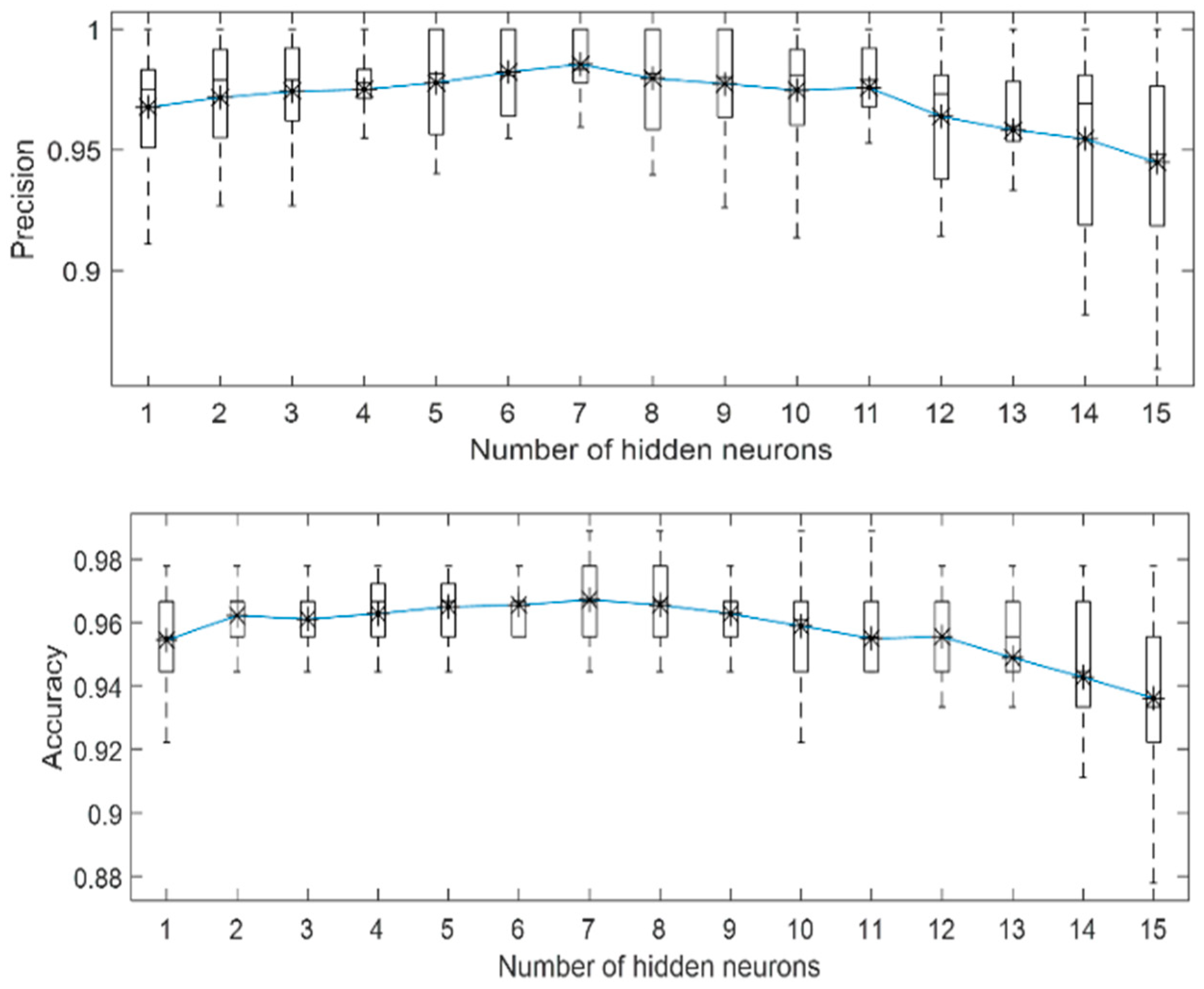
The results obtained from Model 4, as a function of the number of hidden neurons, are shown in the Figure 9:
Analyzing the results obtained for Model 4, it is observed that for the proposed configurations of the ANN model, greater precision and accuracy values were achieved compared to Model 3. In this case, reducing the number of input variables in the model (six inputs instead of eleven used in Model 3) improved the classification performance of the ANN model to predict the corrosion status of stainless steels in biogas environments.
The maximum precision and accuracy values obtained by the model were 0.985 and 0.967, respectively, using seven neurons in the hidden layer. In this case, an excessive number of hidden neurons led to poor classification performance. Comparing these results with those obtained for Model 3, it can be concluded that considering PREN allowed obtaining a more accurate model. Furthermore, according to Lemeshow and Hosmer, Model 4 can be defined as an excellent classifier since the accuracy value was greater than 0.9.

3.3. Influence of Breakdown Potential on Corrosion Modelling of Stainless Steel in Biogas Production

Finally, the objective was to analyze the influence of the breakdown potential of the passive layer obtained from the polarization curve on the classification performance. MODEL 5 was proposed, and its characteristics are specified in Table 6. In this case, the breakdown potential value was not considered an input variable. Compared with the previously proposed models, this approach had the advantage that it allowed us to determine the corrosion status of stainless steel automatically, with no need to carry out electrochemical tests or the microscopic analysis of the material surface. In this case, the model was trained considering as input variables the following ones: stainless steel composition, temperature, type of artificial solution simulating biogas environment, surface finish of the material under study, and the type of localized corrosion (pitting or crevice corrosion).
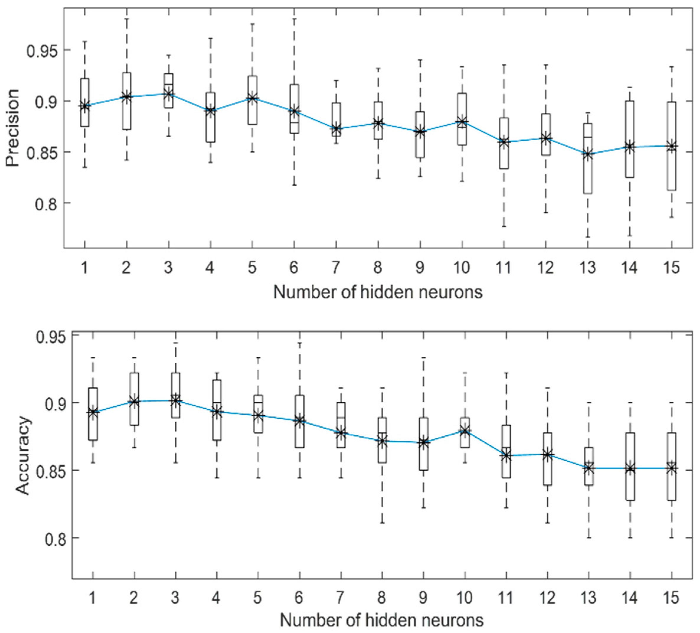
The results for Model 5, in terms of precision and accuracy, are shown in Figure 10:
According to Figure 10, the maximum precision and accuracy values reached for the different configurations proposed for Model 5 were 0.907 and 0.902, respectively. In this case, the optimal configuration was obtained when three neurons were considered in the hidden layer. These results demonstrated that the model showed a good capability to predict the corrosion status of stainless steel for this application automatically. However, the results related to precision and accuracy values were much lower than those obtained for Model 3, where the breakdown potential value was considered an input in the ANN model. This fact emphasizes the importance of considering the breakdown potential value of the passive layer to model the corrosion behaviour of stainless steel in biogas environments.
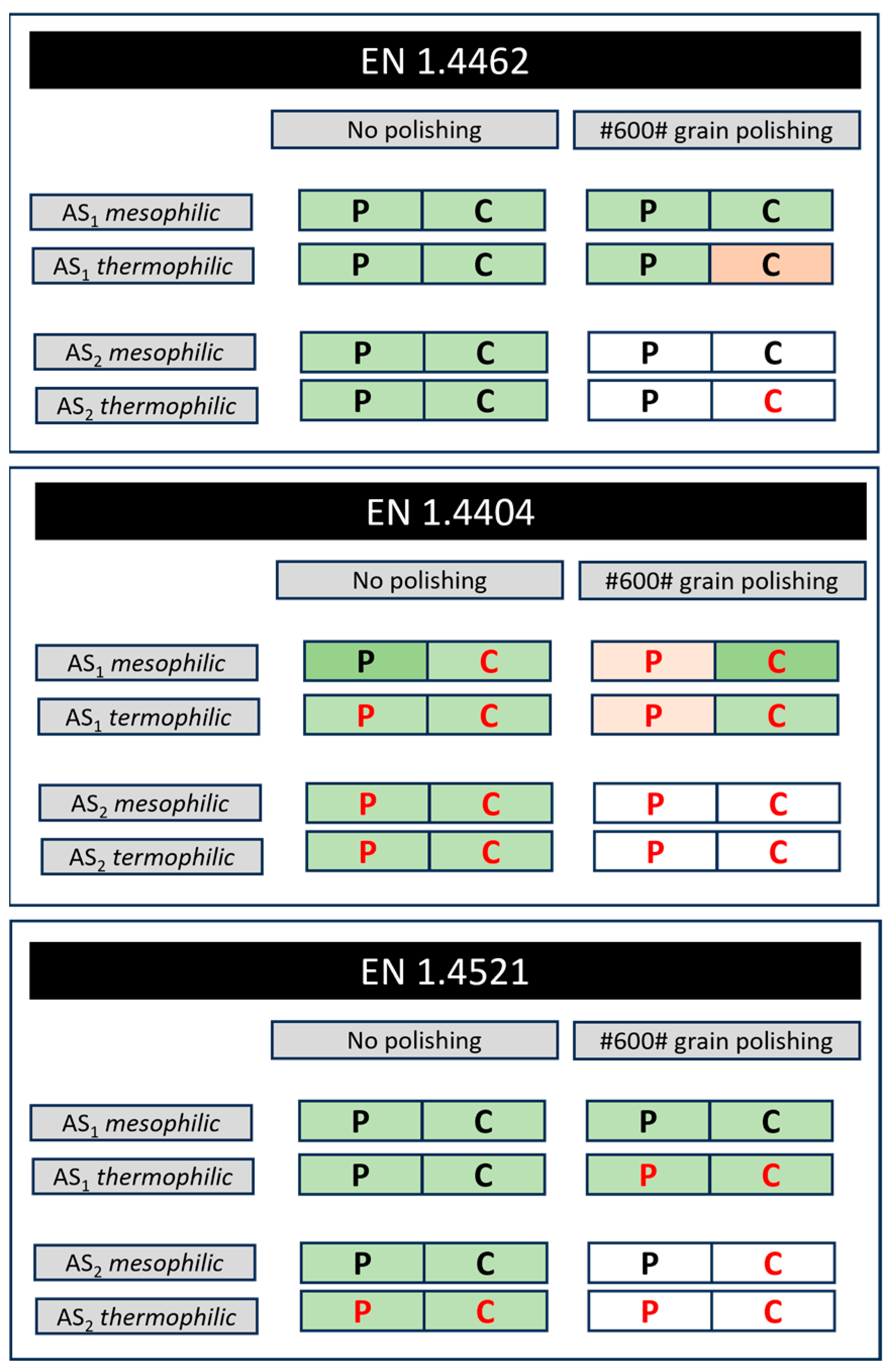
Figure 11 depicts the results obtained from Model 5 using three neurons in the hidden layer. This figure shows the corrosion status predicted by the model under different conditions simulating biogas environments. In this case, following the experimental procedure, the corrosion state predicted by the model will be determined based on the artificial solution (AS1 or AS2), the thermal conditions (mesophilic or thermophilic), and the surface finish. In this case, the corrosion state is represented considering a pitting attack (P) or crevice attack (C). Cases in which the model predicts that the material will not undergo corrosion are shown in black, while cases in which the model predicts that the material will experience corrosion are shown in red. Furthermore, for those cases in which the corrosion state predicted by the model matches the one obtained experimentally, the box is coloured green, while in cases where they do not match, orange is used. While the graph represents the case for three grades of stainless steel (EN 1.4462, EN 1.4404, and EN 1.4521), the model is applicable to any alloy composition of stainless steel within the studied range.

4. Conclusions

In order to minimize the impact of corrosion on the durability of stainless steel structures used in biogas production, different models based on ANN were proposed in this study.
The main objective was to develop an ANN model capable of predicting the corrosion state of stainless steel involved in biogas production. The two most important types of localized corrosion that can affect stainless steel in this type of application were analyzed: pitting and crevice corrosion. The variables considered to model corrosion behaviour were those related to the composition of the material, the breakdown potential of the passive layer obtained from electrochemical tests and the conditions to which the material may be exposed in biogas production (temperature and type of artificial solution simulating the biogas environmental conditions). Different configurations were proposed, concluding the following aspects:
The proposed ANN model presented in this work to predict the corrosion status of the material after electrochemical tests with no need to analyze the material surface microscopically, MODEL 3, showed high classification performance. In this case, the precision and accuracy values obtained were 96.8% and 96.6%, respectively. These values demonstrated the usefulness of Model 3 to predict the corrosion status of the material without resorting to microscopic analysis of its surface and thus reducing the subjectivity in the results. However, the proposed model was not completely automatic; as for new experimental conditions, it was necessary to know the value of the breakdown potential from electrochemical tests since it was defined as input to the model. In order to obtain an automatic model to predict corrosion status, Model 5 was proposed, excluding the breakdown potential value as input for modelling. In this case, the corrosion behaviour of stainless steel could be predicted automatically for new exposure conditions without the need to perform electrochemical tests for the new samples. However, the precision (90.7%) and accuracy (90.2%) of the model decreased compared with Model 3. This result demonstrated the importance of considering the breakdown potential of the passive layer to model corrosion behaviour in biogas environments.
In addition, the composition of the stainless steel considered as input to model corrosion behaviour can be represented by PREN. This index is calculated based on the percentage of the alloying elements. In this way, when PREN was considered as input for modelling, the number of input variables was reduced, improving the classification performance. In this case, for Model 4, the maximum values for precision and accuracy were 98.5% and 96.7%, respectively.
These results showed that ANN-based models could be shown as a useful tool in the design of biodigester since they predict the corrosion behaviour of stainless steel accurately depending on the environmental conditions to which the material will be exposed in biogas production. Therefore, the model allows for selecting the correct grade of stainless steel in biogas production based on the environmental conditions to which it will be exposed.

Author Contributions

M.J.J.-C.: Writing—Review and Editing, Methodology, Software, Formal analysis, Supervision. F.J.G.G.: Conceptualization, Writing—Review and Editing, Methodology. P.Á.G.: Data Curation, Resources. J.D.M.B.: Resources, Validation. All authors have read and agreed to the published version of the manuscript.

Funding

This research was funded by Universidad de Cádiz, grant number, 52004195.

Data Availability Statement

The raw/processed data required to reproduce the above findings cannot be shared at this time as the data also form part of an ongoing study.

Acknowledgments

The authors gratefully acknowledge the financial support provided by the Projects funded by the University of Cadiz (52004195). It has been developed with the support of the European project “Innovative and competitive solutions using stainless steel and adhesive bonding in biogas. (BiogaSS)”, developed partly in ACERINOX EUROPA S.A.U.

Conflicts of Interest

The authors declare that they have no known competing financial interests or personal relationships that could have appeared to influence the work reported in this work.

References

  1. Cesaro, A.; Belgiorno, V. Combined Biogas and Bioethanol Production: Opportunities and Challenges for Industrial Application. Energies 2015, 8, 8121–8144. [Google Scholar] [CrossRef]
  2. Guo, M.; Song, W.; Buhain, J. Bioenergy and biofuels: History, status, and perspective. Renew. Sustain. Energy Rev. 2015, 42, 712–725. [Google Scholar] [CrossRef]
  3. Angelidaki, I.; Treu, L.; Tsapekos, P.; Luo, G.; Campanaro, S.; Wenzel, H.; Kougias, P.G. Biogas upgrading and utilization: Current status and perspectives. Biotechnol. Adv. 2018, 36, 452–466. [Google Scholar] [CrossRef] [PubMed]
  4. Weiland, P. Biogas production: Current state and perspectives. Appl. Microbiol. Biotechnol. 2010, 85, 849–860. [Google Scholar] [CrossRef] [PubMed]
  5. Zhang, Y.; Kawasaki, Y.; Oshita, K.; Takaoka, M.; Minami, D.; Inoue, G.; Tanaka, T. Economic assessment of biogas purification systems for removal of both H2S and siloxane from biogas. Renew. Energy 2021, 168, 119–130. [Google Scholar] [CrossRef]
  6. Koch, G.H.; Brongers, M.P.H.; Thompson, N.G.; Virmani, Y.P.; Payer, J.H. Corrosion Costs and Preventive Strategies in the United States; FHWA: Washingt, DC, USA, 2001.
  7. Bo, T.; Zhu, X.; Zhang, L.; Tao, Y.; He, X.; Li, D.; Yan, Z. A new upgraded biogas production process: Coupling microbial electrolysis cell and anaerobic digestion in single-chamber, barrel-shape stainless steel reactor. Electrochem. Commun. 2014, 45, 67–70. [Google Scholar] [CrossRef]
  8. Ruiz, D.; Miguel, G.S.; Corona, B.; Gaitero, A.; Domínguez, A. Environmental and economic analysis of power generation in a thermophilic biogas plant. Sci. Total. Environ. 2018, 633, 1418–1428. [Google Scholar] [CrossRef]
  9. Bao, L.; Li, K.; Zheng, J.; Zhang, Y.; Zhan, K.; Yang, Z.; Zhao, B.; Ji, V. Surface characteristics and stress corrosion behavior of AA 7075-T6 aluminum alloys after different shot peening processes. Surf. Coat. Technol. 2022, 440, 128481. [Google Scholar] [CrossRef]
  10. Shekari, E.; Khan, F.; Ahmed, S. Economic risk analysis of pitting corrosion in process facilities. Int. J. Press. Vessel. Pip. 2017, 157, 51–62. [Google Scholar] [CrossRef]
  11. NACE International. International Measures of Prevention, Application, and Economics of Corrosion Technologies Study 2012; NACE International: Houston, TX, USA, 2012. [Google Scholar]
  12. Chen, Z.; Gao, L.; Koleva, D.A. Evaluating the stray current corrosion of steel rebar in different layouts. Measurement 2022, 196, 111217. [Google Scholar] [CrossRef]
  13. Ma, C.; Wang, Z.; Behnamian, Y.; Gao, Z.; Wu, Z.; Qin, Z.; Xia, D.-H. Measuring atmospheric corrosion with electrochemical noise: A review of contemporary methods. Measurement 2019, 138, 54–79. [Google Scholar] [CrossRef]
  14. Sanni, O.; Adeleke, O.; Ukoba, K.; Ren, J.; Jen, T.-C. Application of machine learning models to investigate the performance of stainless steel type 904 with agricultural waste. J. Mater. Res. Technol. 2022, 20, 4487–4499. [Google Scholar] [CrossRef]
  15. Hao, J.-Z.; Xu, S.-A.; Xu, J.-J.; Cao, H.-L.; Miao, H. Modeling and optimization of the corrosion resistance of Cr-free and Cr-based chemical conversion coatings on nickel foil by artificial neural network and response surface method. Mater. Today Commun. 2023, 36, 106858. [Google Scholar] [CrossRef]
  16. Akbarzadeh, S.; Akbarzadeh, K.; Ramezanzadeh, M.; Naderi, R.; Mahdavian, M.; Olivier, M.-G. Corrosion resistance enhancement of a sol-gel coating by incorporation of modified carbon nanotubes: Artificial neural network (ANN) modeling and experimental explorations. Prog. Org. Coat. 2023, 174, 107296. [Google Scholar] [CrossRef]
  17. Moses, A.; Chen, D.; Wan, P.; Wang, S. Prediction of electrochemical corrosion behavior of magnesium alloy using machine learning methods. Mater. Today Commun. 2023, 37, 107285. [Google Scholar] [CrossRef]
  18. Kumari, P.; Halim, S.Z.; Kwon, J.S.-I.; Quddus, N. An integrated risk prediction model for corrosion-induced pipeline incidents using artificial neural network and Bayesian analysis. Process Saf. Environ. Prot. 2022, 167, 34–44. [Google Scholar] [CrossRef]
  19. Woldesellasse, H.; Tesfamariam, S. Data augmentation using conditional generative adversarial network (cGAN): Application for prediction of corrosion pit depth and testing using neural network. J. Pipeline Sci. Eng. 2023, 3, 100091. [Google Scholar] [CrossRef]
  20. Duan, Y.; Ma, L.; Qi, H.; Li, R.; Li, P. Developed constitutive models, processing maps and microstructural evolution of Pb-Mg-10Al-0.5B alloy. Mater. Charact. 2017, 129, 353–366. [Google Scholar] [CrossRef]
  21. Pintos, S.; Queipo, N.V.; de Rincón, O.T.; Rincón, A.; Morcillo, M. Artificial neural network modeling of atmospheric corrosion in the MICAT project. Corros. Sci. 2000, 42, 35–52. [Google Scholar] [CrossRef]
  22. Díaz, V.; López, C.; Rivero, S. Low carbon steel corrosion damage prediction in rural and urban environments. Rev. De Met. 2003, 39, 188–193. [Google Scholar] [CrossRef]
  23. Díaz, V.; López, C. Discovering key meteorological variables in atmospheric corrosion through an artificial neural network model. Corros. Sci. 2007, 49, 949–962. [Google Scholar] [CrossRef]
  24. Silva, R.; Guerreiro, J.; Loula, A. A study of pipe interacting corrosion defects using the FEM and neural networks. Adv. Eng. Softw. 2007, 38, 868–875. [Google Scholar] [CrossRef]
  25. Kenny, E.D.; Paredes, R.S.C.; de Lacerda, L.A.; Sica, Y.C.; de Souza, G.P.; Lázaris, J. Artificial neural network corrosion modeling for metals in an equatorial climate. Corros. Sci. 2009, 51, 2266–2278. [Google Scholar] [CrossRef]
  26. Halama, M.; Kreislova, K.; Van Lysebettens, J. Prediction of Atmospheric Corrosion of Carbon Steel Using Artificial Neural Network Model in Local Geographical Regions. Corrosion 2011, 67, 065004-1–065004-6. [Google Scholar] [CrossRef]
  27. Lin, H.-T.; Lo, C.-M.; Lin, M.-D. Application of Artificial Neural Networks on Predicting Corrosion Rates of Carbon Steel in Taiwan Industrial Zones. Adv. Intell. Syst. Res. 2017, 132, 278–282. [Google Scholar] [CrossRef]
  28. Tran, N.-L.; Nguyen, T.-H.; Phan, V.-T.; Nguyen, D.-D. A Machine Learning-Based Model for Predicting Atmospheric Corrosion Rate of Carbon Steel. Adv. Mater. Sci. Eng. 2021, 2021, 6967550. [Google Scholar] [CrossRef]
  29. Kim, H.-S.; Park, S.-J.; Seo, S.-M.; Yoo, Y.-S.; Jeong, H.-W.; Jang, H. Regression analysis of high-temperature oxidation of Ni-based superalloys using artificial neural network. Corros. Sci. 2021, 180, 109207. [Google Scholar] [CrossRef]
  30. Zhu, Y.; Macdonald, D.D.; Qiu, J.; Urquidi-Macdonald, M. Corrosion of rebar in concrete. Part III: Artificial Neural Network analysis of chloride threshold data. Corros. Sci. 2021, 185, 109438. [Google Scholar] [CrossRef]
  31. Wang, C.; Li, W.; Xin, G.; Wang, Y.; Xu, S.; Fan, M. Novel method for prediction of corrosion current density of gas pipeline steel under stray current interference based on hybrid LWQPSO-NN model. Measurement 2022, 200, 111592. [Google Scholar] [CrossRef]
  32. Li, Q.; Wang, D.; Zhao, M.; Yang, M.; Tang, J.; Zhou, K. Modeling the corrosion rate of carbon steel in carbonated mixtures of MDEA-based solutions using artificial neural network. Process Saf. Environ. Prot. 2021, 147, 300–310. [Google Scholar] [CrossRef]
  33. Soomro, A.A.; Mokhtar, A.A.; Kurnia, J.C.; Lashari, N.; Lu, H.; Sambo, C. Integrity assessment of corroded oil and gas pipelines using machine learning: A systematic review. Eng. Fail. Anal. 2022, 131, 105810. [Google Scholar] [CrossRef]
  34. Yang, J.; Li, R.; Chen, L.; Hu, Y.; Dou, Z. Research on equipment corrosion diagnosis method and prediction model driven by data. Process Saf. Environ. Prot. 2022, 158, 418–431. [Google Scholar] [CrossRef]
  35. Entezari, A.; Aslani, A.; Zahedi, R.; Noorollahi, Y. Artificial intelligence and machine learning in energy systems: A bibliographic perspective. Energy Strat. Rev. 2023, 45, 101017. [Google Scholar] [CrossRef]
  36. Akhshik, M.; Bilton, A.; Tjong, J.; Singh, C.V.; Faruk, O.; Sain, M. Prediction of greenhouse gas emissions reductions via machine learning algorithms: Toward an artificial intelligence-based life cycle assessment for automotive lightweighting. Sustain. Mater. Technol. 2022, 31, e00370. [Google Scholar] [CrossRef]
  37. Kaab, A.; Sharifi, M.; Mobli, H.; Nabavi-Pelesaraei, A.; Chau, K.-W. Combined life cycle assessment and artificial intelligence for prediction of output energy and environmental impacts of sugarcane production. Sci. Total. Environ. 2019, 664, 1005–1019. [Google Scholar] [CrossRef]
  38. Ryan, M.P.; Williams, D.E.; Chater, R.J.; Hutton, B.M.; McPhail, D.S. Why stainless steel corrodes. Nature 2002, 415, 770–774. [Google Scholar] [CrossRef]
  39. Sedriks, A.J. Corrosion of Stainless Steel; John Wiley & Sons: Hoboken, NJ, USA, 1996. [Google Scholar]
  40. Vargel, C. Crevice Corrosion. In Corrosion of Aluminium; Elsevier: Amsterdam, The Netherlands, 2020; pp. 267–271. [Google Scholar] [CrossRef]
  41. Blackwood, D.J.; Lim, C.S.; Teo, S.L.; Hu, X.; Pang, J. Macrofouling induced localized corrosion of stainless steel in Singapore seawater. Corros. Sci. 2017, 129, 152–160. [Google Scholar] [CrossRef]
  42. Mele, C.; Bozzini, B. Localised corrosion processes of austenitic stainless steel bipolar plates for polymer electrolyte membrane fuel cells. J. Power Sources 2010, 195, 3590–3596. [Google Scholar] [CrossRef]
  43. Jiménez-Come, M.J.; Martín, M.d.l.L.; Matres, V.; Baladés, J.D.M. The use of artificial neural networks for modelling pitting corrosion behaviour of EN 1.4404 stainless steel in marine environment: Data analysis and new developments. Corros. Rev. 2020, 38, 339–353. [Google Scholar] [CrossRef]
  44. Jiménez-Come, M.J.; Turias, I.J.; Ruiz-Aguilar, J.J. A two-stage model based on artificial neural networks to determine pitting corrosion status of 316L stainless steel. Corros. Rev. 2016, 34, 113–125. [Google Scholar] [CrossRef]
  45. ASTM International. Annual Book of ASTM Standards; American Society for Testing & Materials: West Conshohocken, PA, USA, 2004. [Google Scholar]
  46. Deng, B.; Jiang, Y.; Gong, J.; Zhong, C.; Gao, J.; Li, J. Critical pitting and repassivation temperatures for duplex stainless steel in chloride solutions. Electrochim. Acta 2008, 53, 5220–5225. [Google Scholar] [CrossRef]
  47. White, H. Learning in Artificial Neural Networks: A Statistical Perspective. Neural Comput. 1989, 1, 425–464. [Google Scholar] [CrossRef]
  48. Rumelhart, D.E.; Hinton, G.E.; Williams, R.J. Learning representations by back-propagating errors. Nature 1986, 323, 533–536. [Google Scholar] [CrossRef]
  49. Lippmann, R. An introduction to computing with neural nets. IEEE Assp Mag. 1987, 4, 4–22. [Google Scholar] [CrossRef]
  50. Lourakis, M.I.A. A brief description of the Levenberg-Marquardt algorithm implemented by levmar. Found. Res. Technol. 2005, 11, 1–6. [Google Scholar]
  51. David, W.H.; Stanley, L. Applied Survival Analysis; Elsevier Science Inc.: New York, NY, USA, 2000. [Google Scholar] [CrossRef]
  52. Fawcett, T. An Introduction to ROC analysis. Pattern Recogn. Lett. 2006, 27, 861–874. [Google Scholar] [CrossRef]
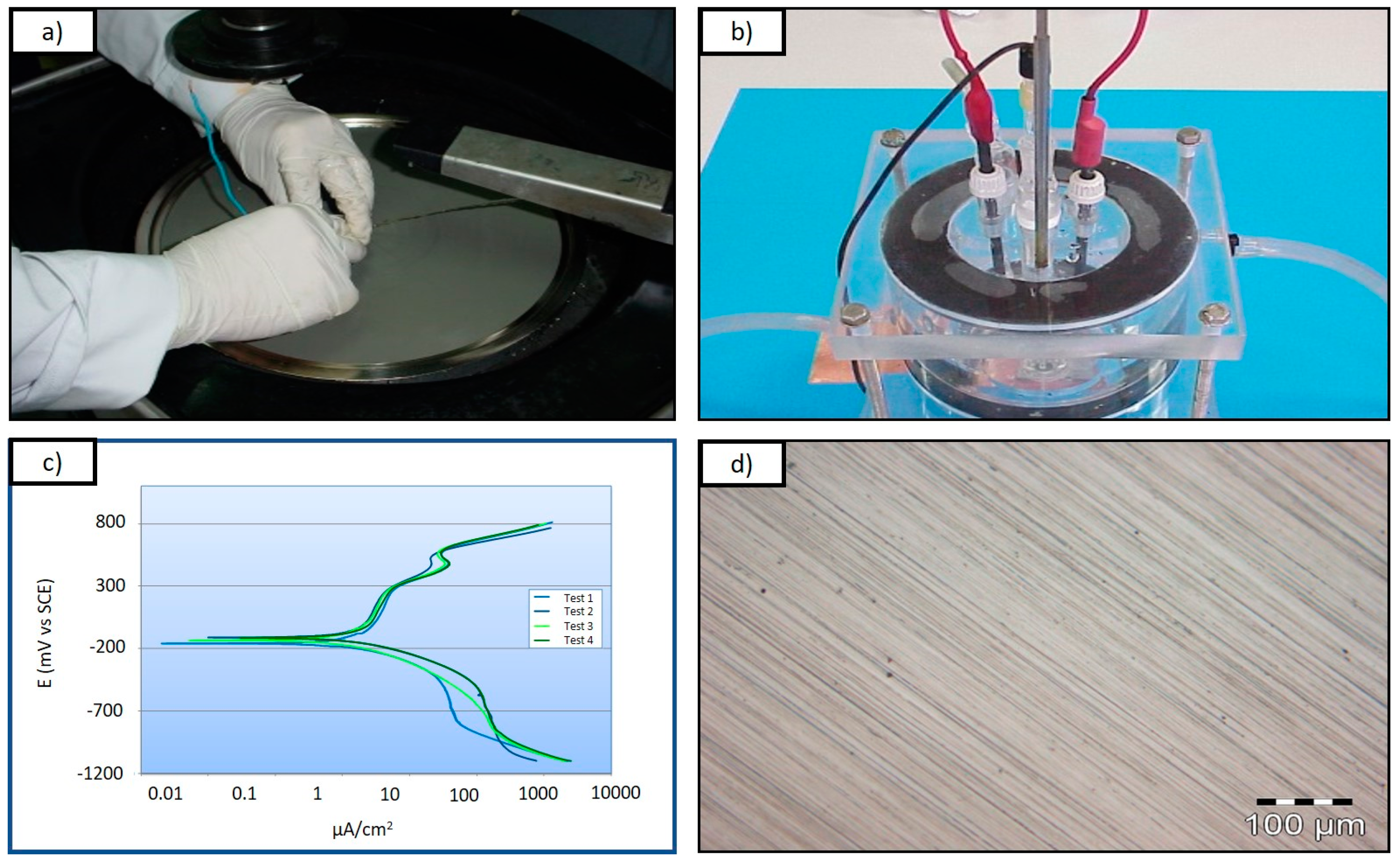
Figure 1. Experimental procedure of stainless steel EN 1.4462: (a) polishing, (b) electrochemical cell design, (c) potentiodynamic curves, (d) microscopic analysis.
Metals 13 01811 g001
Figure 2. Mathematical model of an artificial neuron.
Metals 13 01811 g002
Figure 3. Structure for the proposed ANN model (Model 1) to predict the pitting corrosion status of stainless steel in biogas production. The input variables considered in this case were alloy composition, Eb (breakdown potential of passive layer), Temperature, AS (type of artificial solution simulating biogas environment), and SF (surface finish of the material).
Metals 13 01811 g003
Figure 4. Methodology proposed to model the corrosion behaviour of stainless steel in biogas environments.
Metals 13 01811 g004
Figure 5. Influence of the number of hidden neurons in ANN models on precision and accuracy results for Model 1. Mean values (20 repetitions) for each case are pointed out with an asterisk.
Metals 13 01811 g005
Figure 6. Influence of the number of hidden neurons in ANN models on precision and accuracy results (Model 2). Mean values for each case are pointed out with an asterisk.
Metals 13 01811 g006
Figure 7. Influence of the number of hidden neurons in ANN models on precision and accuracy results (Model 3). Mean values for each case are pointed out with an asterisk.
Metals 13 01811 g007
Figure 8. ROC graph for the different configurations of Model 1, Model 2, and Model 3.
Metals 13 01811 g008
Figure 9. Influence of the number of hidden neurons in ANN models on precision and accuracy results (Model 4). Mean values for each case are pointed out with an asterisk.
Metals 13 01811 g009
Figure 10. Influence of the number of hidden neurons in ANN models on precision and accuracy results (Model 5). Mean values for each case are pointed out with an asterisk.
Metals 13 01811 g010
Figure 11. Corrosion behaviour predicted by the model under different conditions simulating biogas environments, considering different artificial solutions (AS1 or AS2), thermal conditions (mesophilic or thermophilic), and the surface finish. In this case, the corrosion state is represented considering a pitting attack (P) or crevice attack (C). Corrosion cases are represented with red letters, while no-corrosion cases are indicated with black letters.
Metals 13 01811 g011
Table 1. Stainless steel composition for experimental tests.
Stainless Steel GradeCr (%)Mo (%)N (%)Mn (%)Ti (%)Nb (%)
EN 1.440416.712.0180.0381.2910.0160.016
EN 1.446222.8923.2790.16191.3970.0340.011
EN 1.448219.940.2230.13744.0160.0250.006
EN 1.400311.450.010.01150.5470.0150.006
EN 1.457116.8012.0660.01341.5780.3010.008
EN 1.450918.4920.0510.02350.430.1480.393
EN 1.452118.5551.9990.0240.5070.1270.416
EN 1.431817.7440.0890.1441.2580.0020.007
Table 2. Artificial solutions conditions.
Reagentg/LAS 1AS 2
Sodium Sulphate, Na2SO312.67XX
Ammonium Chloride, NH4Cl69.81XX
Ammonium carbonate, (NH4)2CO315.13XX
Sodium Acetate Trihydrate, NaCH3COOH·3H2O17.06XX
Hydrogen chloride, HCl, from FeCl2 desulfuration7.31--X
pH range 8.2–8.56.6–7.2
Table 3. Confusion matrix for corrosion modelling.
Target Status
Positive
(Corrosion Pattern)
Negative
(No-Corrosion Pattern)
Classification results
PositiveTP (True Positive)FP (False Positive)
NegativeFN (False Negative)TN (True Negative)
Table 4. Structure of the proposed ANN model to model localized corrosion of stainless steel in biogas production. The inputs variables considered in this case were: alloy composition, Eb (breakdown potential of passive layer), Temperature, AS (type of artificial solution simulating biogas environment), and SF (surface finish of the material).
IdentityCorrosion Type Input NeuronsOutput Neurons:
Model 1Pitting 10 units:
%Cr, %Mo, %N, %Mn, %Ti, %Nb, Eb, T, AS, SF
2 units:
1: corrosion pattern
0: no-corrosion pattern
Model 2Crevice10 units:
%Cr, %Mo, %N, %Mn, %Ti, %Nb, Eb, T, AS, SF
2 units:
1: corrosion pattern
0: no-corrosion pattern
Model 3Pitting and Crevice 11 units:
%Cr, %Mo, %N, %Mn, %Ti, %Nb, Eb, T, AS, SF, corrosion type (pitting or crevice)
2 units:
1: corrosion pattern
0: no-corrosion pattern
Table 5. Structure of the proposed ANN model to model localized corrosion of stainless steel in biogas production (MODEL 4).
IdentityCorrosion Type Input NeuronsOutput Neurons:
Model 4Pitting and Crevice 6 units:
PREN, Eb, T, AS, SF,
corrosion type (pitting or crevice)
2 units:
1: corrosion pattern
0: no-corrosion pattern
Table 6. Structure of the proposed ANN model to model localized corrosion of stainless steel in biogas production (MODEL 5).
IdentityCorrosion Type Input NeuronsOutput Neurons:
Model 5Pitting and Crevice 10 units:
%Cr, %Mo, %N, %Mn, %Ti, %Nb, T, AS, SF, corrosion type (pitting or crevice)
2 units:
1: corrosion pattern
0: no-corrosion pattern
Disclaimer/Publisher’s Note: The statements, opinions and data contained in all publications are solely those of the individual author(s) and contributor(s) and not of MDPI and/or the editor(s). MDPI and/or the editor(s) disclaim responsibility for any injury to people or property resulting from any ideas, methods, instructions or products referred to in the content.