
Fracture Mechanics Modeling of Fatigue Behaviors of Adhesive-Bonded Aluminum Alloy Components


Abstract
:1. Introduction
2. Analytical Fracture Mechanics Modeling
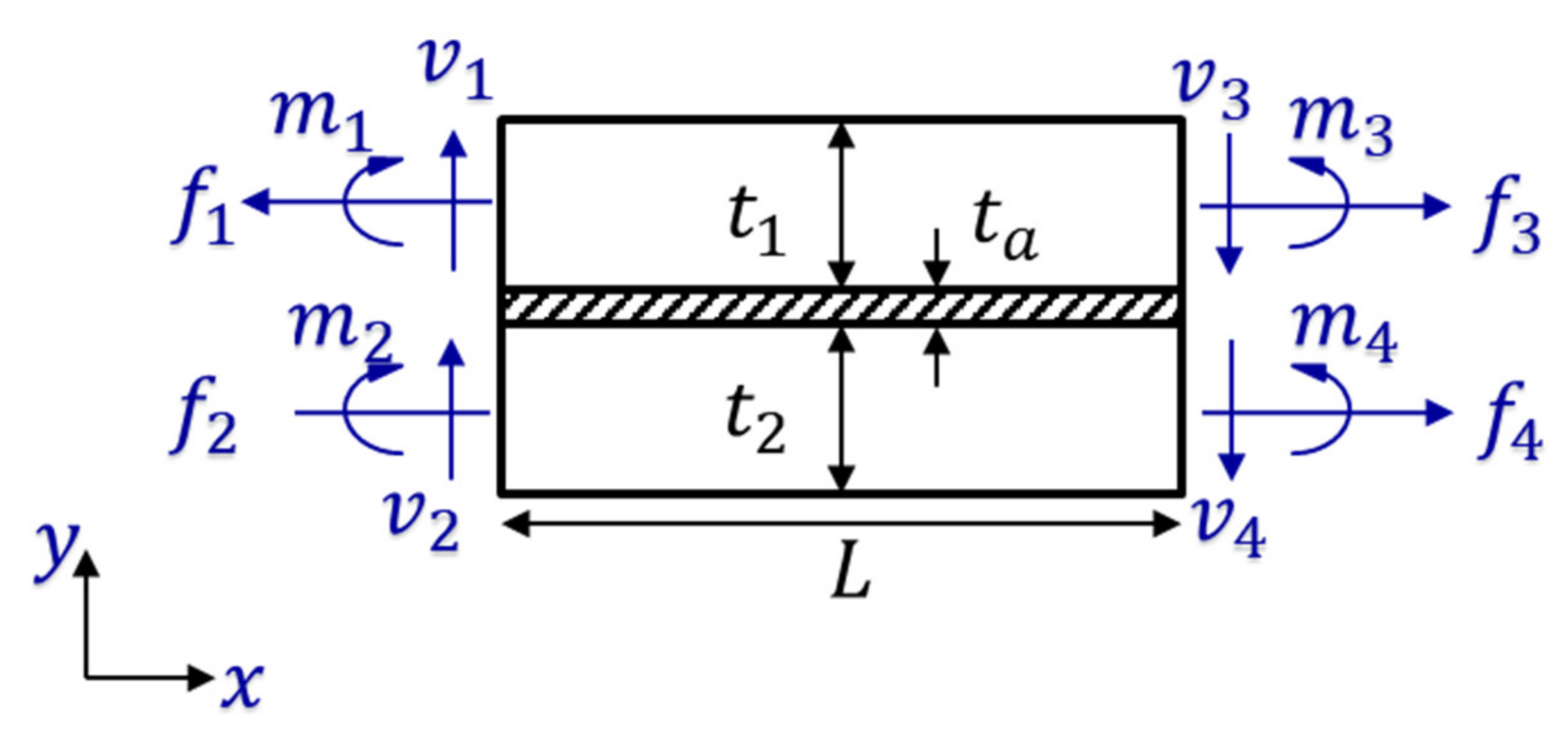
2.1. Problem Idealization
2.2. Closed-Form Stress Intensity Factor Solutions
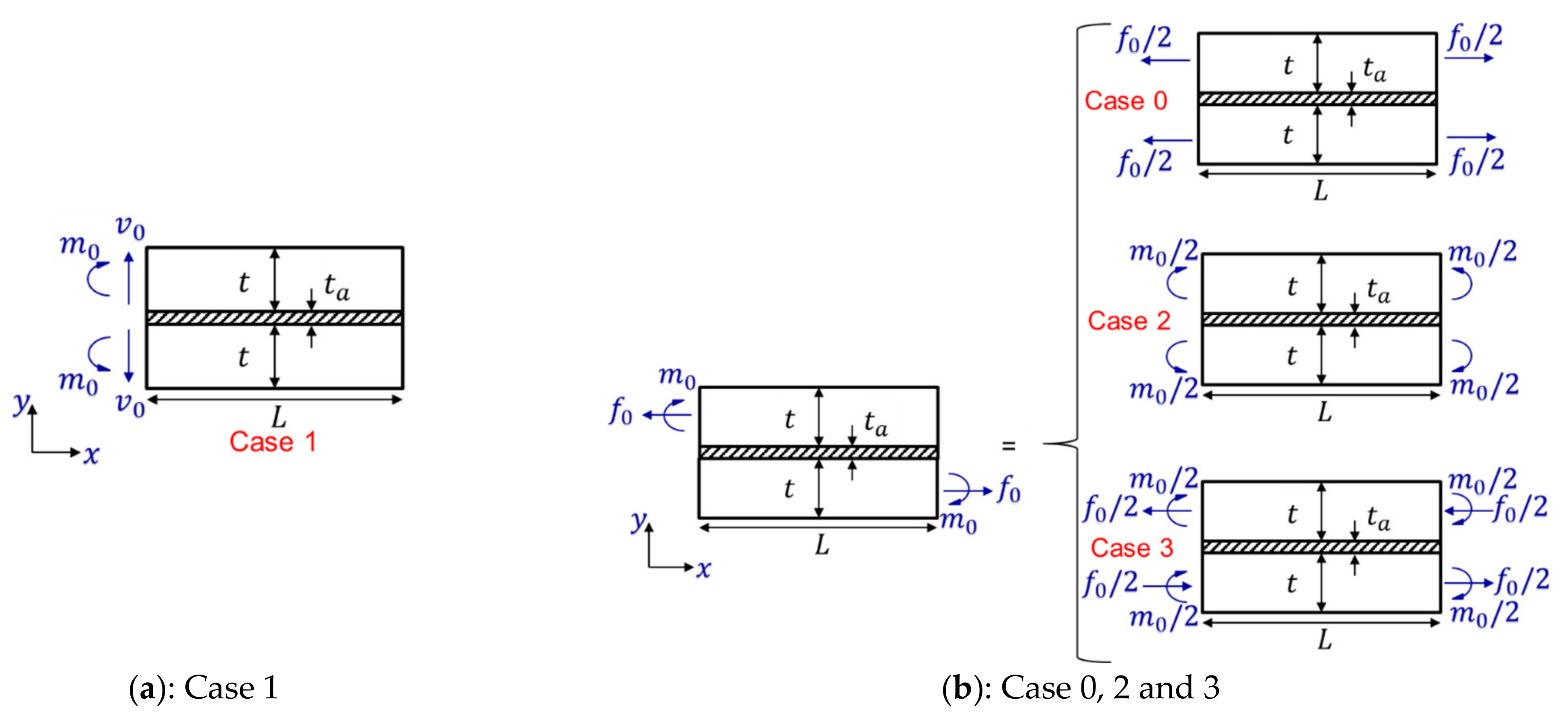
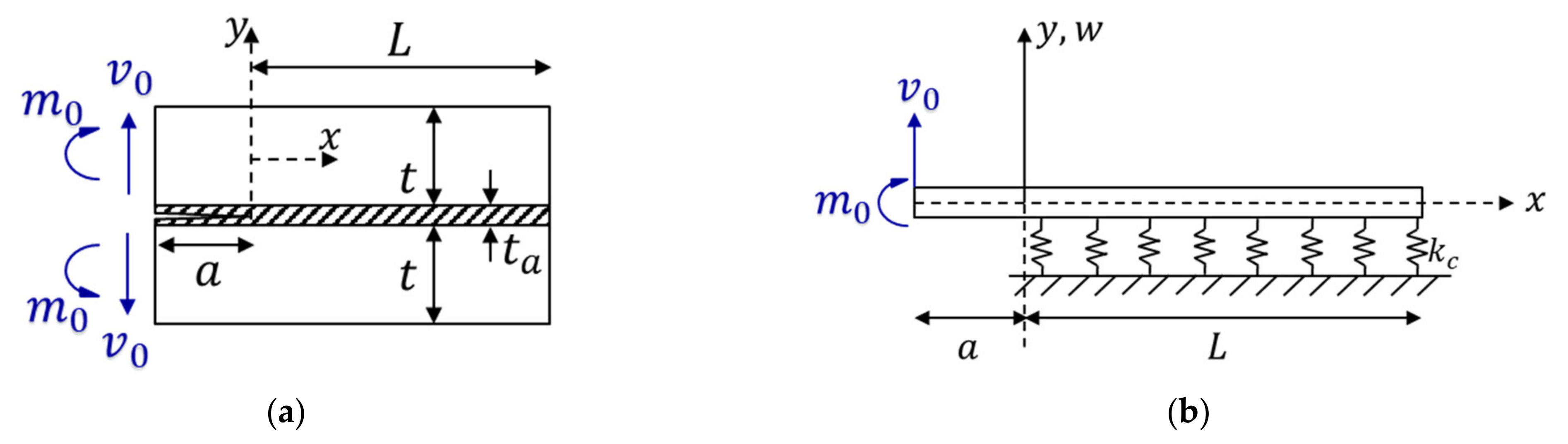
2.2.1. Case 1
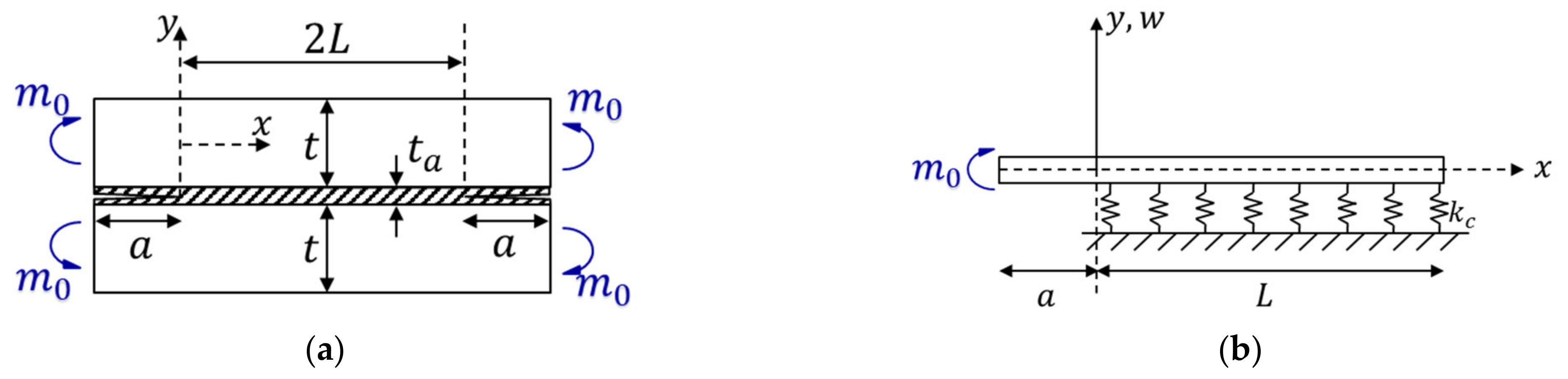
2.2.2. Case 2
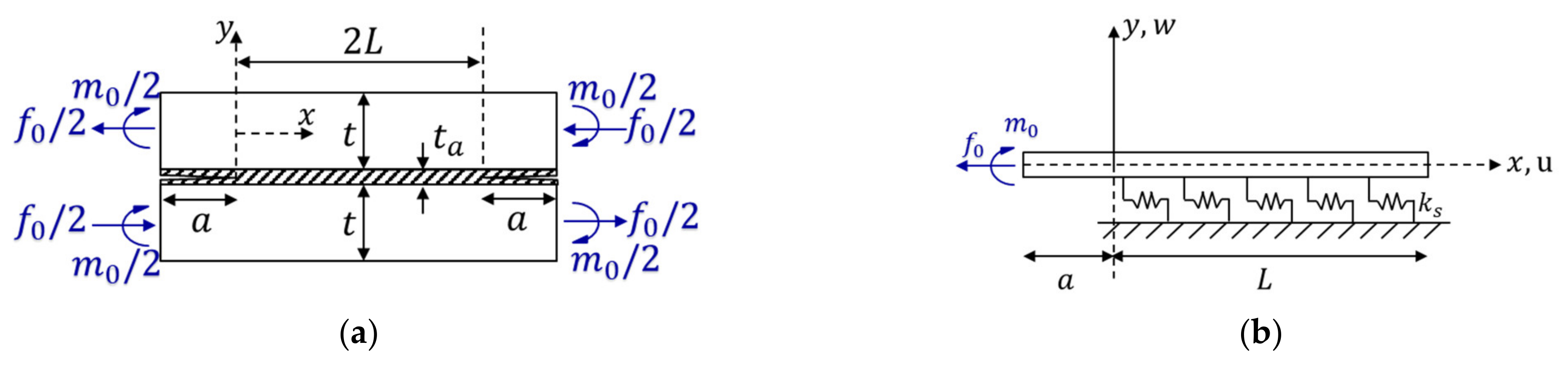
2.2.3. Case 3
2.3. Analytical Results and Implications
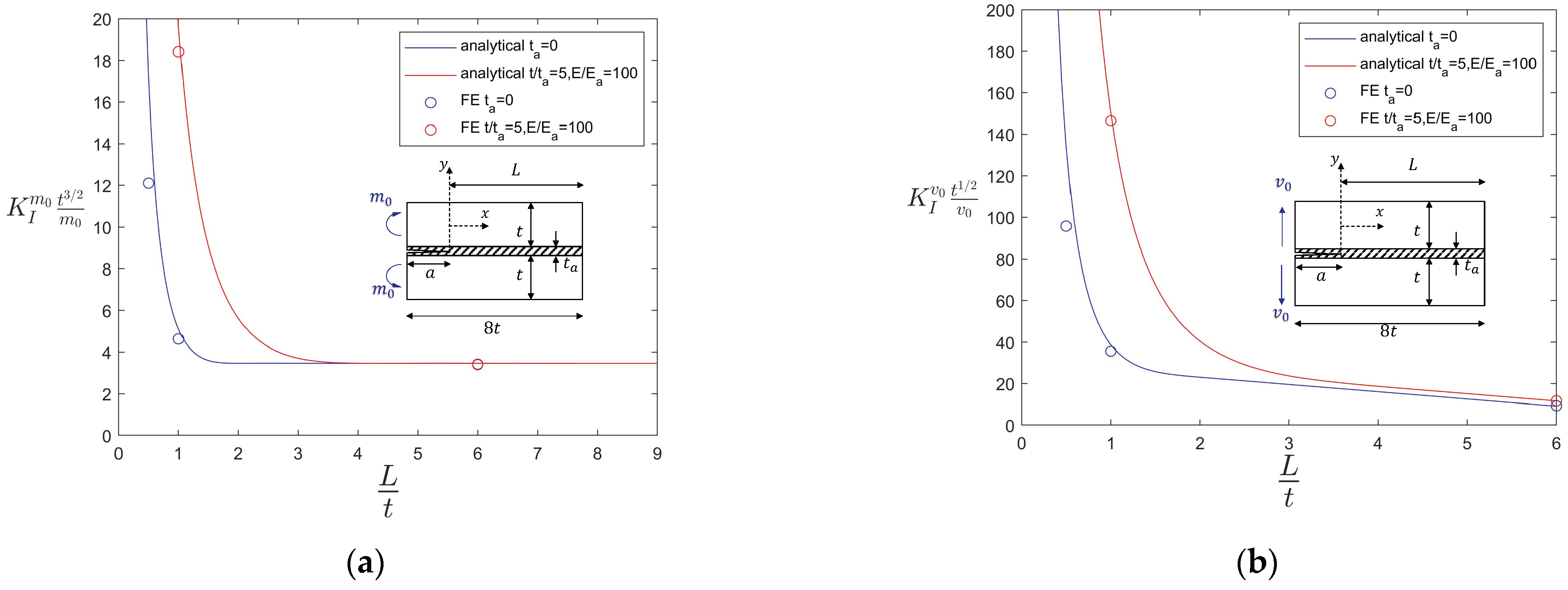
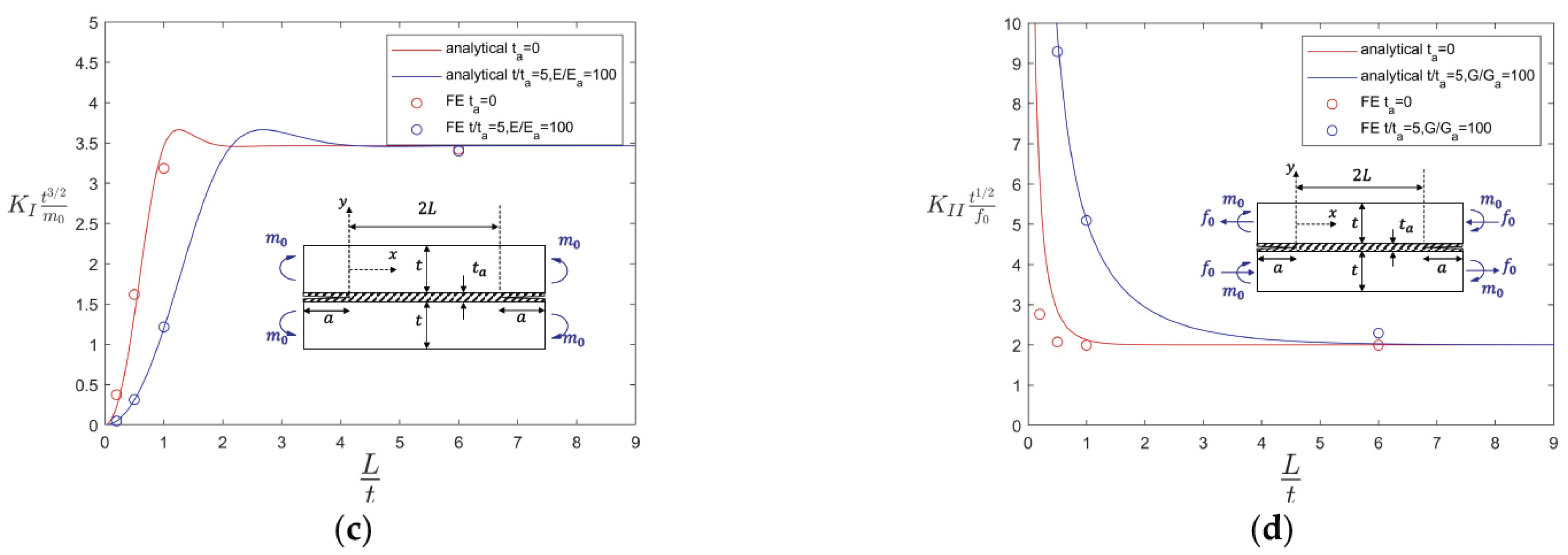
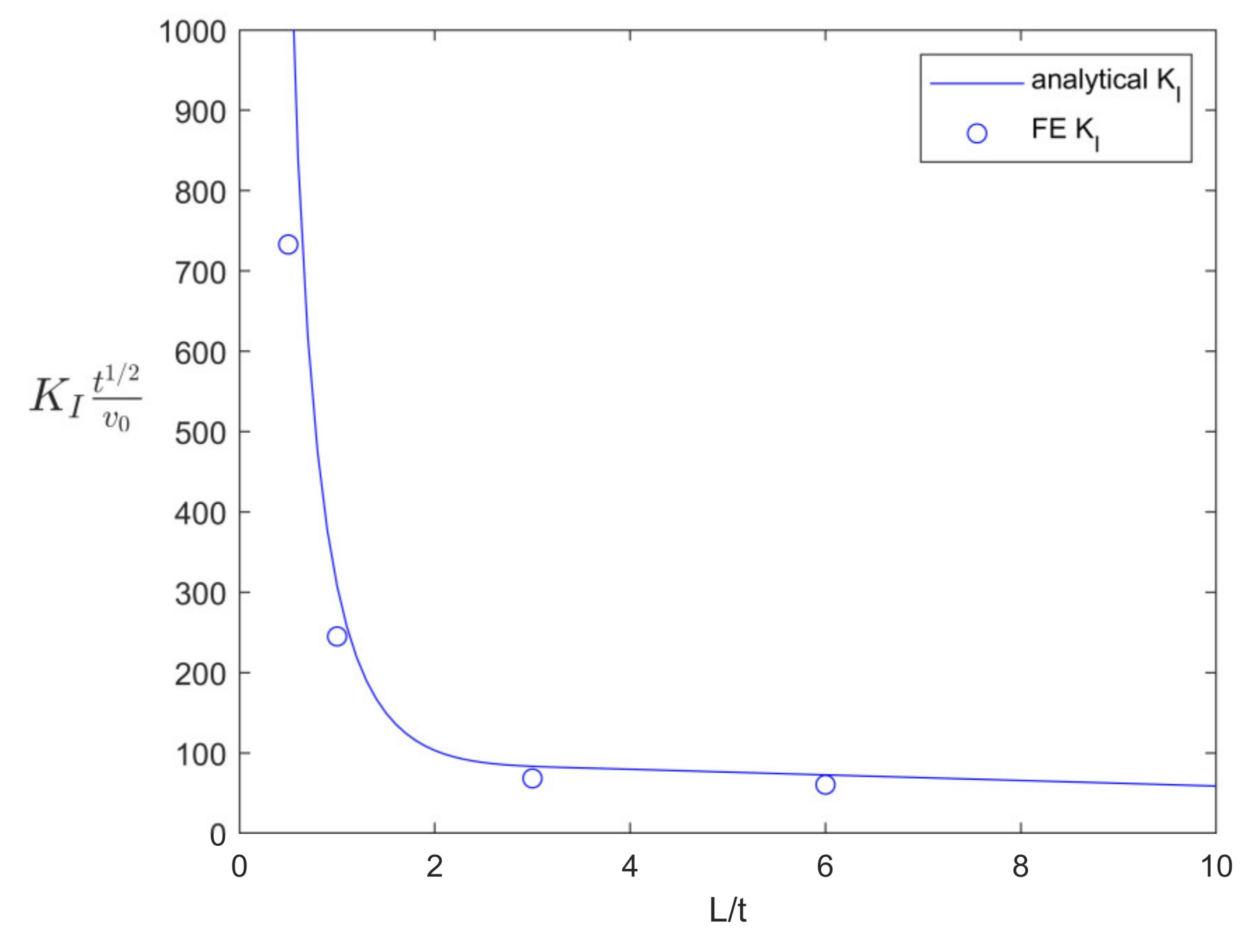
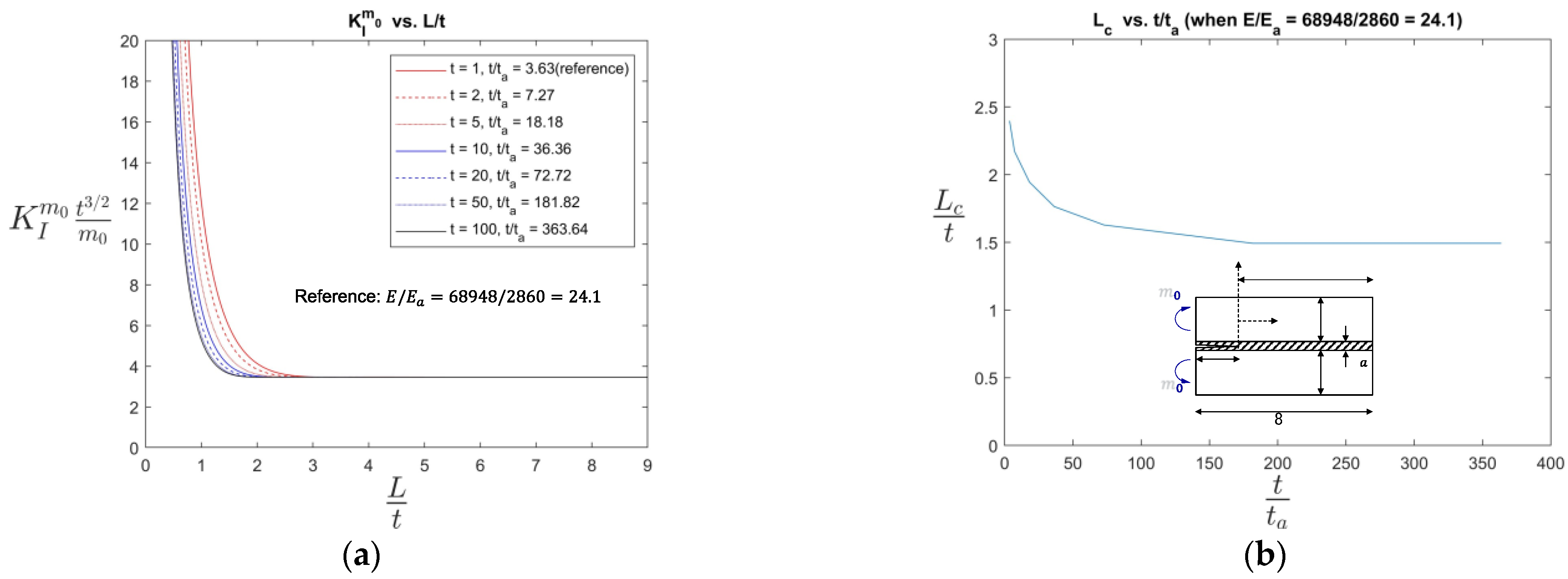
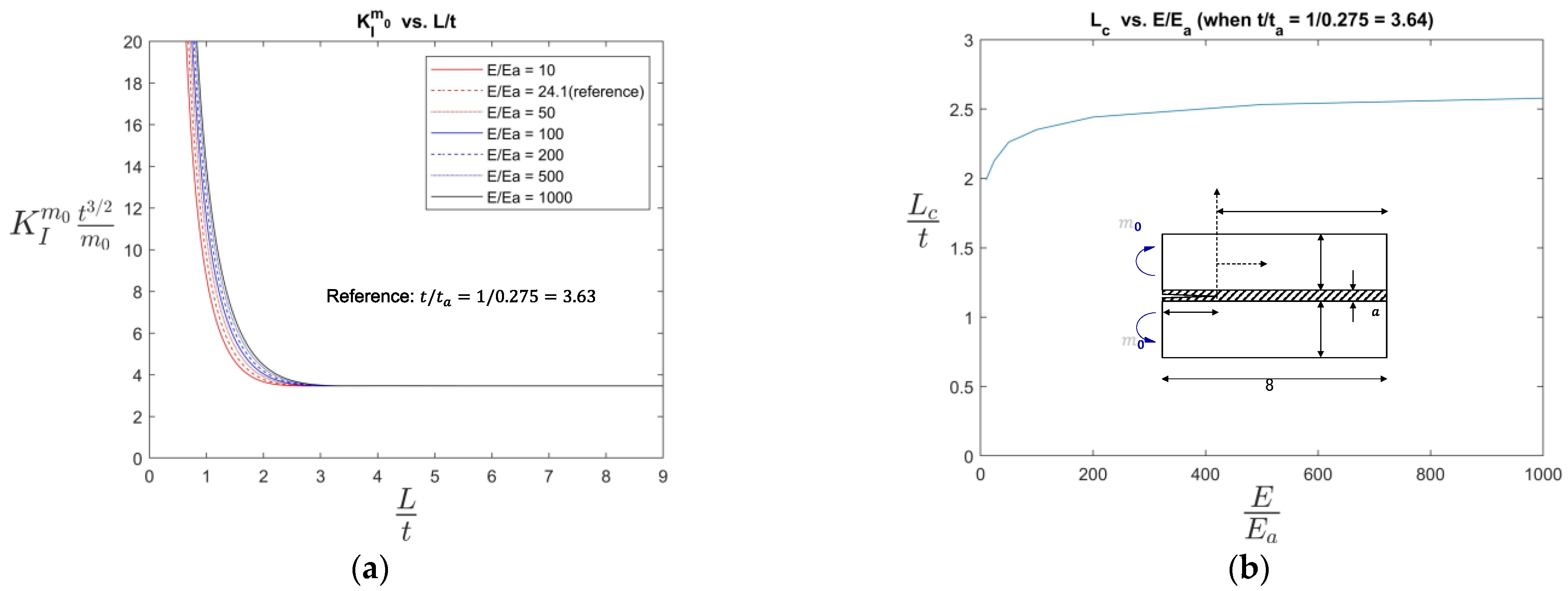
- In all cases, when L/t was large enough (e.g., 3), the SIF values approached a constant value of low magnitude (see Figure 7a,c,d) or a constant slope (see Figure 7b). These results suggest that there exists a threshold or critical value beyond which an additional bond length increase offers little in return in reducing the SIFs.
- When the was smaller than about 3, the SIFs in Cases 1 (Figure 7a,b) and 3 (Figure 7d) increased rapidly, indicating that in this regime, the bond length was too small to ensure an adequate load-carrying capacity of the joint. The only exception to the above observations was that Case 2 exhibited a decrease in the SIF as approached 0. This trend makes sense, as shown in Figure 5, in that under symmetric moment loading, the crack opening action rapidly diminished as approached zero.
- When the adhesive layer ( was considered, the non-dimensional variable , , and showed a noticeable influence on the non-dimensional SIFs. When the adhesive layer was thin (i.e., small) or stiff (i.e., , the SIF results approached those without considering an adhesive layer (i.e., and vice versa.
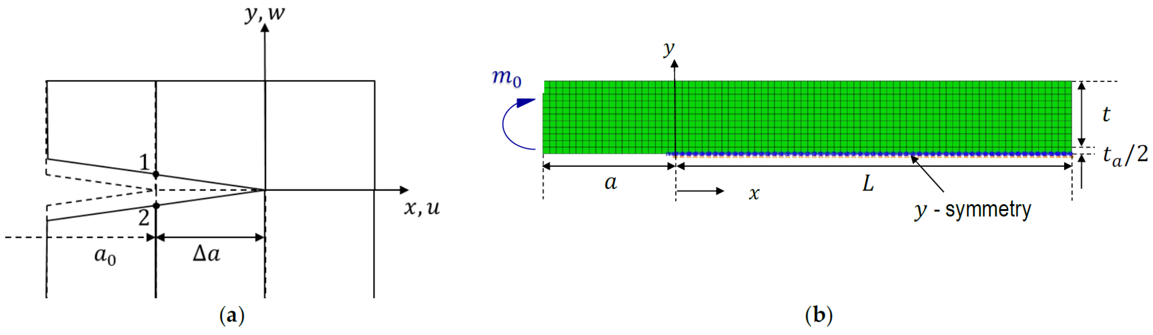
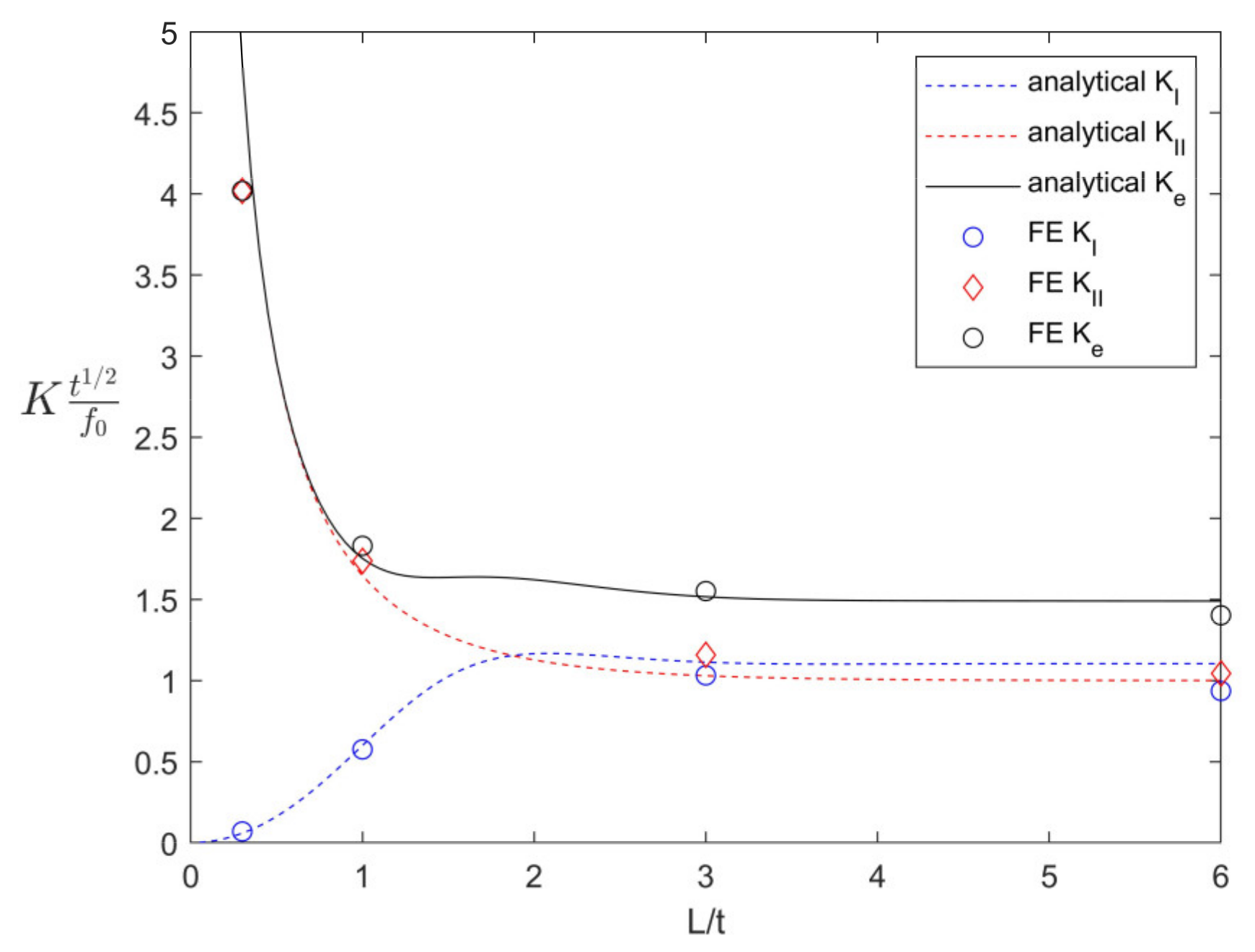
2.4. FE Validations
3. Applications in Fatigue Test Data Analysis
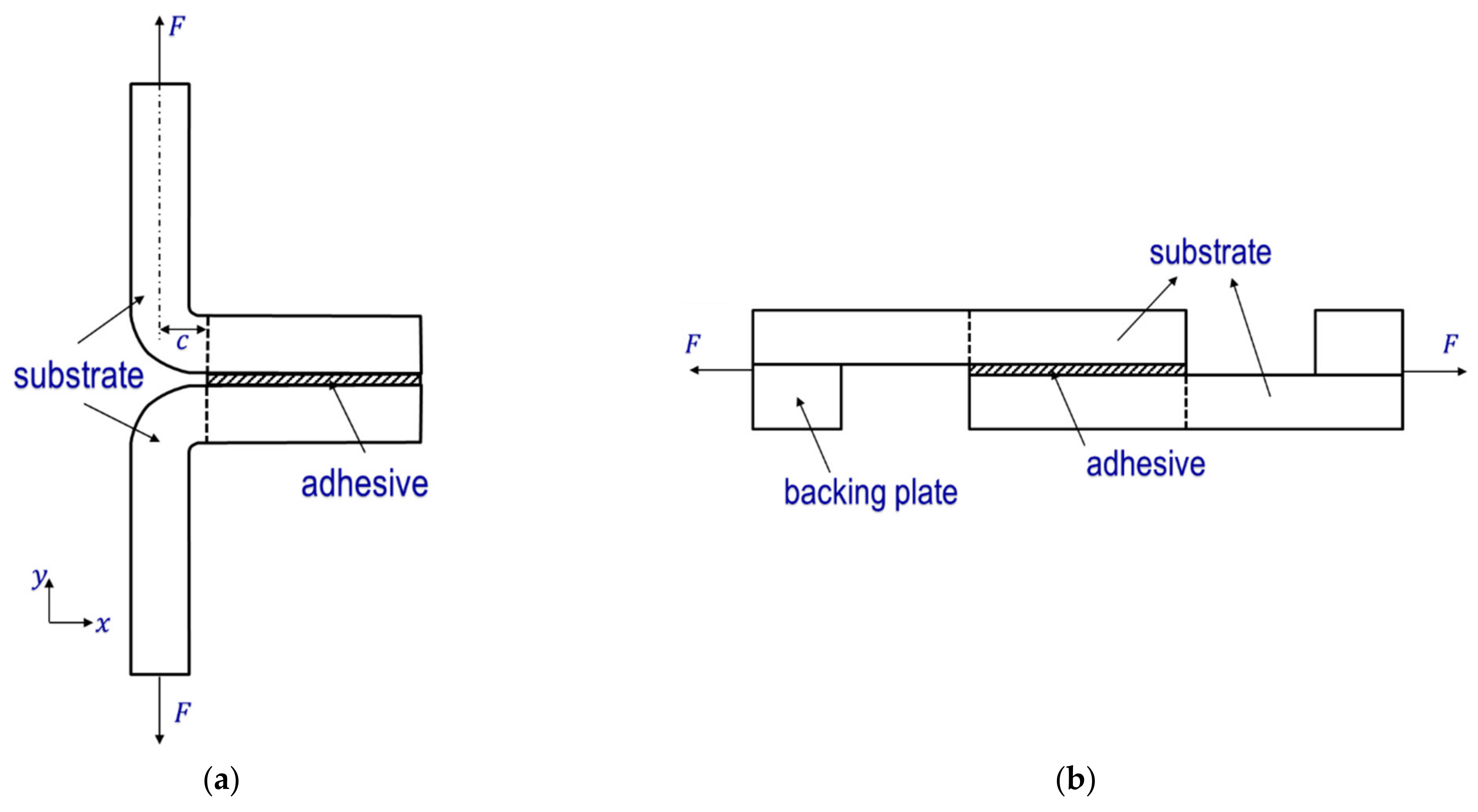
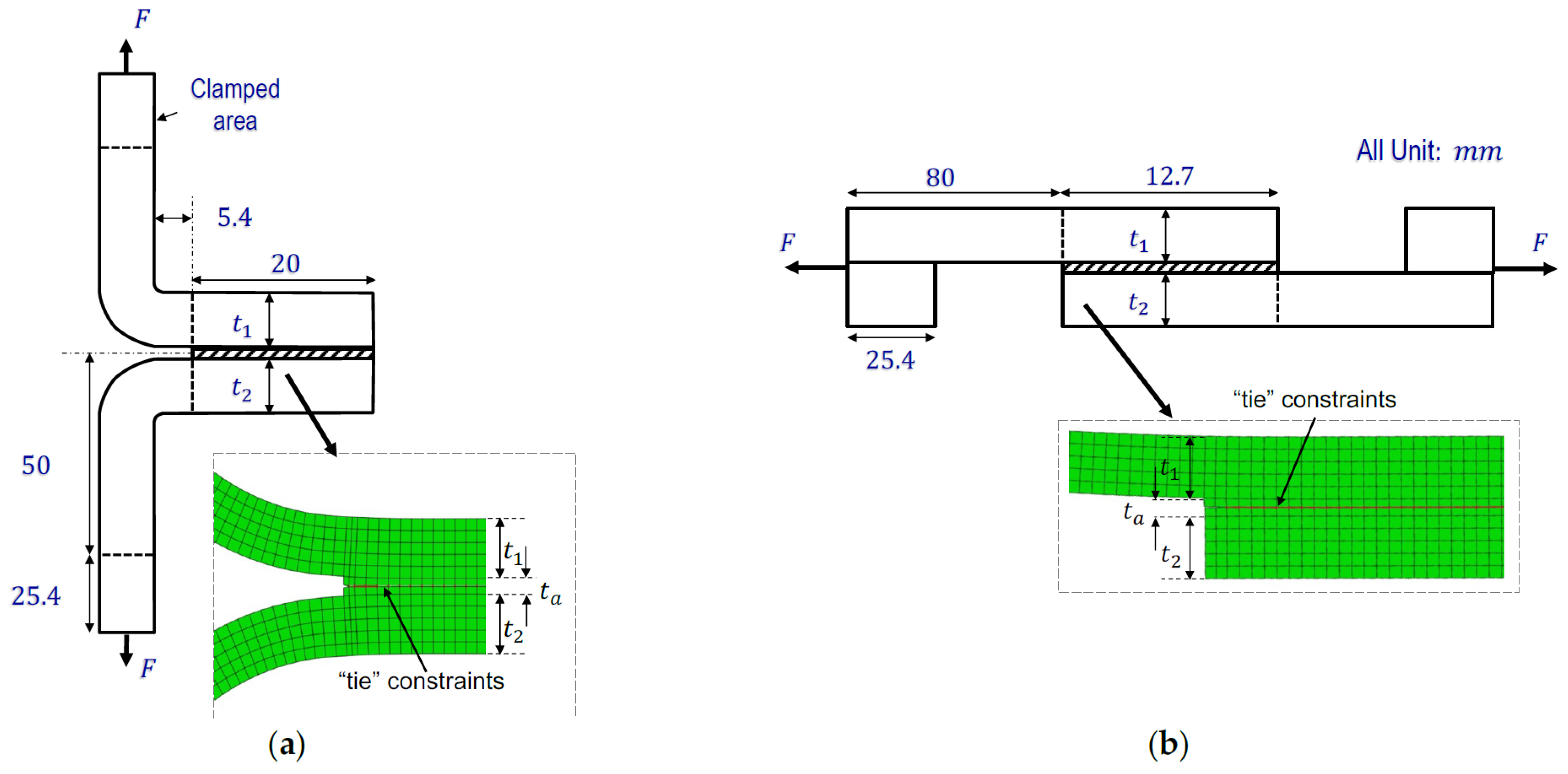
3.1. Fatigue Test Details
3.2. SIFs for Coach-Peel Test Specimens
3.3. SIFs for Lap-Shear Test Specimens
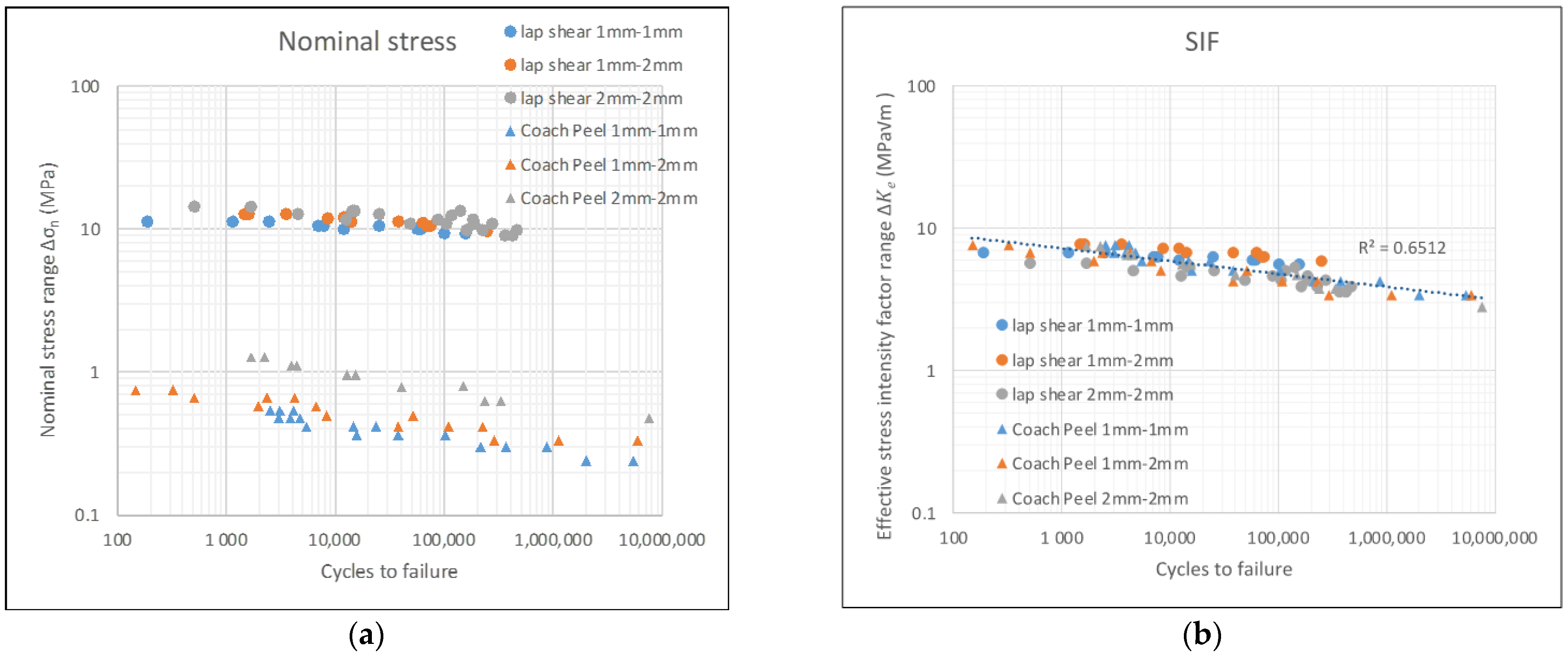
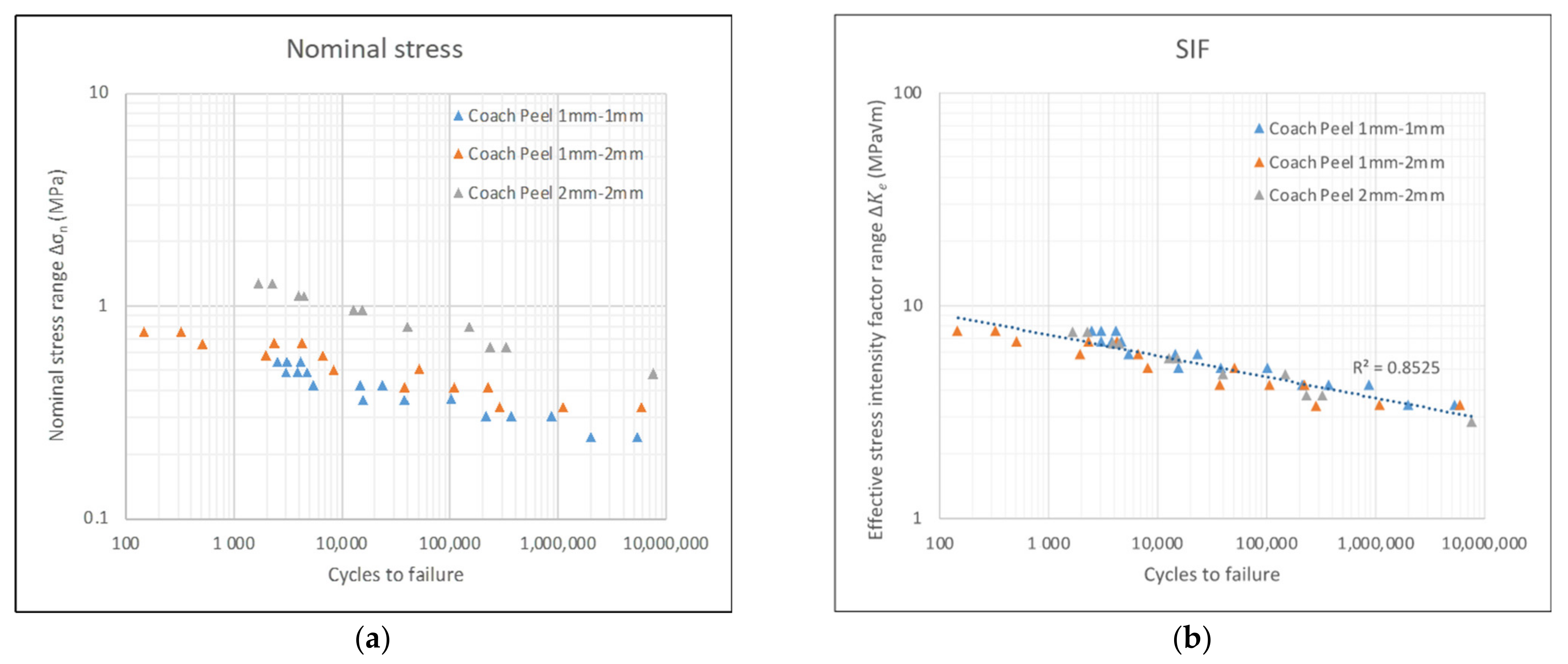
3.4. Fatigue Test Data Correlation Using SIFs
4. Discussions
4.1. Existence of Critical Bond Length
4.2. as a Fatigue Parameter
5. Conclusions
Author Contributions
Funding
Institutional Review Board Statement
Informed Consent Statement
Data Availability Statement
Acknowledgments
Conflicts of Interest
Appendix A. Derivation of Composite Spring Constant
Appendix A.1. Spring Constants Corresponding to Cases 1 and 2

Appendix A.2. Composite Shear Spring Constant Corresponding to Case 3

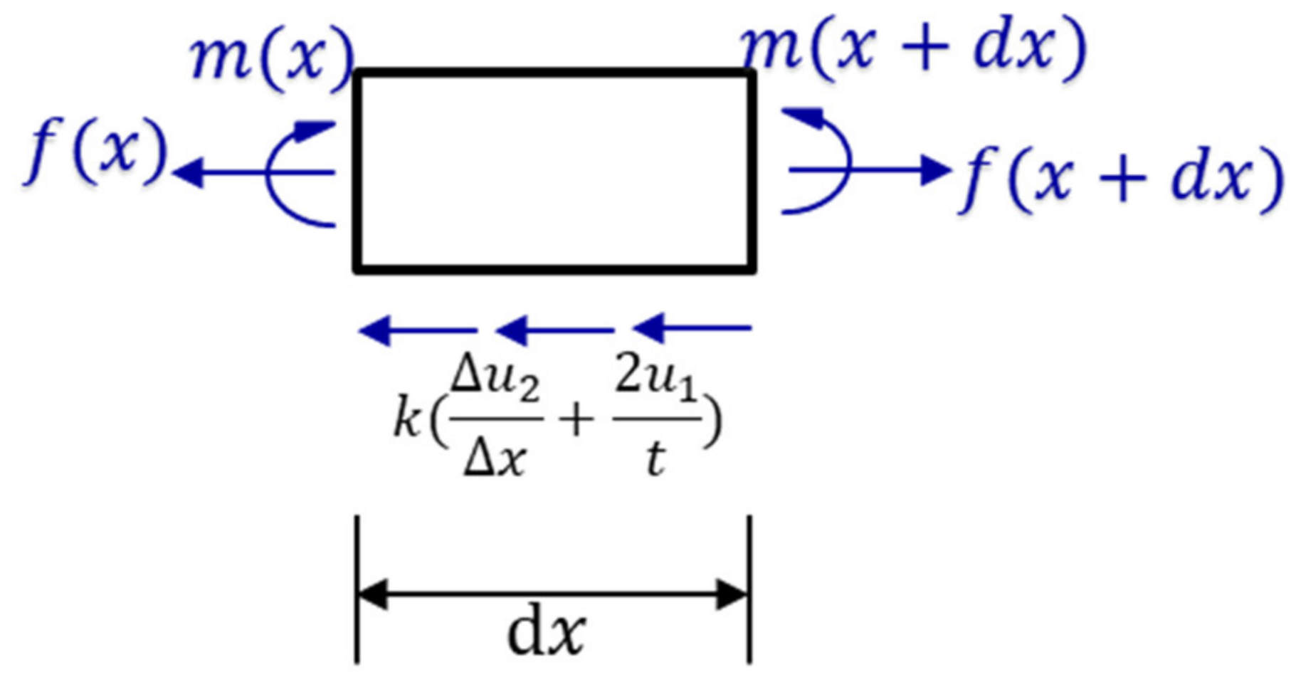
Appendix B. Elastic Foundation Solution with Shear Spring
References
- Chen, Q.; Guo, H.; Avery, K.; Su, X.; Kang, H. Fatigue performance and life estimation of automotive adhesive joints using a fracture mechanics approach. Eng. Fract. Mech. 2017, 172, 73–89. [Google Scholar] [CrossRef]
- Blanco, D.; Rubio, E.M.; Marín, M.M.; Davim, J.P. Advanced materials and multi-materials applied in aeronautical and automotive fields: A systematic review approach. Procedia CIRP 2021, 99, 196–201. [Google Scholar] [CrossRef]
- Lambiase, F.; Scipioni, S.I.; Lee, C.J.; Ko, D.C.; Liu, F. A State-of-the-Art Review on Advanced Joining Processes for Metal-Composite and Metal-Polymer Hybrid Structures. Materials 2021, 14, 1890. [Google Scholar] [CrossRef] [PubMed]
- Liu, F.; Dong, P. Directly and Reliably Welding Plastic to Metal. Weld. J. 2022, 101, 45. [Google Scholar]
- Dong, P. Quantitative weld quality acceptance criteria: An enabler for structural lightweighting and additive manufacturing. Weld. J. 2020, 99, 39S–51S. [Google Scholar] [CrossRef]
- Liu, F.C.; Dong, P.; Lu, W.; Sun, K. On formation of AlOC bonds at aluminum/polyamide joint interface. Appl. Surf. Sci. 2019, 466, 202–209. [Google Scholar] [CrossRef]
- Liu, F.C.; Dong, P.; Pei, X. A high-speed metal-to-polymer direct joining technique and underlying bonding mechanisms. J. Mater. Process. Technol. 2020, 280, 116610. [Google Scholar] [CrossRef]
- Liu, F.C.; Dong, P.; Zhang, J.; Lu, W.; Taub, A.; Sun, K. Alloy amorphization through nanoscale shear localization at Al-Fe interface. Mater. Today Phys. 2020, 15, 100252. [Google Scholar] [CrossRef]
- Liu, F.; Zhang, Y.; Dong, P. Large area friction stir additive manufacturing of intermetallic-free aluminum-steel bimetallic components through interfacial amorphization. J. Manuf. Process. 2022, 73, 725–735. [Google Scholar] [CrossRef]
- Ha, D.W.; Jeon, G.W.; Shin, J.S.; Jeong, C.Y. Mechanical properties of steel-aluminum multi-materials using a structural adhesive. Mater. Today Commun. 2020, 25, 101552. [Google Scholar] [CrossRef]
- Kinloch, A.; Korenberg, C.; Tan, K.T.; Watts, J. The Durability of Structural Adhesive Joints. In Proceedings of the 7th European Adhesion Conference—EURADH 2004, Freiberg, Germany, 1 September 2004. [Google Scholar]
- Gledhill, R.A.; Kinloch, A.J.; Shaw, S.J. A Model for Predicting Joint Durability. J. Adhes. 2007, 11, 3–15. [Google Scholar] [CrossRef]
- Volkersen, O. Die Niektraftverteilung in Zugbeanspruchten mit Konstanten Laschenquerschritten. Luftfahrtforschung 1938, 15, 41–47. [Google Scholar]
- Goland, M.; Buffalo, N.Y.; Reissner, E. The Stresses in Cemented Joints. J. Appl. Mech. 1944, 11, A17–A27. [Google Scholar] [CrossRef]
- Anyfantis, K.N.; Tsouvalis, N.G. Loading and fracture response of CFRP-to-steel adhesively bonded joints with thick adherents—Part I: Experiments. Compos. Struct. 2013, 96, 850–857. [Google Scholar] [CrossRef]
- Davies, P.; Sohier, L.; Cognard, J.Y.; Bourmaud, A.; Choqueuse, D.; Rinnert, E.; Créac’hcadec, R. Influence of adhesive bond line thickness on joint strength. Int. J. Adhes. Adhes. 2009, 29, 724–736. [Google Scholar] [CrossRef] [Green Version]
- Marzi, S.; Biel, A.; Stigh, U. On experimental methods to investigate the effect of layer thickness on the fracture behavior of adhesively bonded joints. Int. J. Adhes. Adhes. 2011, 31, 840–850. [Google Scholar] [CrossRef]
- Boutar, Y.; Naïmi, S.; Mezlini, S.; Da Silva, L.F.M.; Hamdaoui, M.; Ben Sik Ali, M. Effect of adhesive thickness and surface roughness on the shear strength of aluminium one-component polyurethane adhesive single-lap joints for automotive applications. J. Adhes. Sci. Technol. 2016, 30, 1913–1929. [Google Scholar] [CrossRef]
- Monteiro, J.; Akhavan-Safar, A.; Carbas, R.; Marques, E.; Goyal, R.; El-Zein, M.; da Silva, L. Influence of mode mixity and loading conditions on the fatigue crack growth behaviour of an epoxy adhesive. Fatigue Fract. Eng. Mater. Struct. 2019, 43, 308–316. [Google Scholar] [CrossRef]
- Wah, T. Stress Distribution in a Bonded Anisotropic Lap Joint. J. Eng. Mater. Technol. 1973, 95, 174–181. [Google Scholar] [CrossRef]
- Pirvics, J. Two dimensional displacement-stress distributions in adhesive bonded composite structures. J. Adhes. 1974, 6, 207–228. [Google Scholar] [CrossRef]
- Crocombe, A.D.; Bigwood, D.A. Development of a full elasto-plastic adhesive joint design analysis. J. Strain Anal. Eng. Des. 1992, 27, 211–218. [Google Scholar] [CrossRef]
- Adams, R.D.; Mallick, V. A method for the stress analysis of lap joints. J. Adhes. 1992, 38, 199–217. [Google Scholar] [CrossRef]
- Yang, C.; Pang, S.S. Stress-Strain Analysis of Single-Lap Composite Joints Under Tension. J. Eng. Mater. Technol. 1996, 118, 247–255. [Google Scholar] [CrossRef]
- Frostig, Y.; Thomsen, O.T.; Mortensen, F. Analysis of Adhesive-Bonded Joints, Square-End, and Spew-Fillet—High-Order Theory Approach. J. Eng. Mech. 1999, 125, 1298–1307. [Google Scholar] [CrossRef]
- Sawa, T.; Liu, J.; Nakano, K.; Tanaka, J. Two-dimensional stress analysis of single-lap adhesive joints of dissimilar adherends subjected to tensile loads. J. Adhes. Sci. Technol. 2000, 14, 43–66. [Google Scholar] [CrossRef]
- Mortensen, F.; Thomsen, O.T. Analysis of adhesive bonded joints: A unified approach. Compos. Sci. Technol. 2002, 62, 1011–1031. [Google Scholar] [CrossRef]
- Renton, W.J.; Vinson, J.R. The Efficient Design of Adhesive Bonded Joints. J. Adhes. 1975, 7, 175–193. [Google Scholar] [CrossRef]
- Pascoe, J.A.; Alderliesten, R.C.; Benedictus, R. Methods for the prediction of fatigue delamination growth in composites and adhesive bonds—A critical review. Eng. Fract. Mech. 2013, 112–113, 72–96. [Google Scholar] [CrossRef]
- Srinivas, S. Analysis of Bonded Joints NASA Technical Note; NASA Langley Research Center: Hampton, VA, USA, 1975. [Google Scholar]
- Allman, D.J. A theory for elastic stresses in adhesive bonded lap joints. Q. J. Mech. Appl. Math. 1977, 30, 415–436. [Google Scholar] [CrossRef]
- Ojalvo, I.U.; Eidinoff, H.L. Bond thickness effects upon stresses in single-lap adhesive joints. AIAA J. 1978, 16, 204–211. [Google Scholar] [CrossRef]
- Delale, F.; Erdogan, F.; Aydinoglu, M.N. Stresses in Adhesively Bonded Joints: A Closed-Form Solution. J. Compos. Mater. 1981, 15, 249–271. [Google Scholar] [CrossRef] [Green Version]
- Bigwood, D.A.; Crocombe, A.D. Elastic analysis and engineering design formulae for bonded joints. Int. J. Adhes. Adhes. 1989, 9, 229–242. [Google Scholar] [CrossRef]
- Cheng, S.; Chen, D.; Shi, Y. Analysis of AdhesiveBonded Joints with Nonidentical Adherends. J. Eng. Mech. 1991, 117, 605–623. [Google Scholar] [CrossRef]
- Dillard, D.A. Applying Fracture Mechanics to Adhesive Bonds; Woodhead Publishing: Cambridge, UK, 2021; ISBN 9780128199541. [Google Scholar]
- Lyathakula, K.R.; Yuan, F.G. A probabilistic fatigue life prediction for adhesively bonded joints via ANNs-based hybrid model. Int. J. Fatigue 2021, 151, 106352. [Google Scholar] [CrossRef]
- Reddy Lyathakula, K.; Yuan Karthik Reddy Lyathakula, F.-G.; Yuan, F.-G. Probabilistic fatigue life prediction for adhesively bonded joints via surrogate model. In Proceedings of the Sensors and Smart Structures Technologies for Civil, Mechanical, and Aerospace Systems 2021, Online, 22 March 2021; Volume 11591, pp. 152–162. [Google Scholar] [CrossRef]
- Akhavan-Safar, A.; Marques, E.A.S.; Carbas, R.J.C.; da Silva, L.F.M. Cohesive Zone Modelling for Fatigue Life Analysis of Adhesive Joints; Springer Briefs in Applied Sciences and Technology; Springer International Publishing: Cham, Switzerland, 2022; ISBN 978-3-030-93141-4. [Google Scholar]
- Zhang, L.; Dong, P.; Wang, Y.; Mei, J. A Coarse-Mesh hybrid structural stress method for fatigue evaluation of Spot-Welded structures. Int. J. Fatigue 2022, 164, 107109. [Google Scholar] [CrossRef]
- Kanninen, M.F. An augmented double cantilever beam model for studying crack propagation and arrest. Int. J. Fract. 1973, 9, 83–92. [Google Scholar] [CrossRef]
- Mei, J.; Dong, P.; Kalnaus, S.; Jiang, Y.; Wei, Z. A path-dependent fatigue crack propagation model under non-proportional modes I and III loading conditions. Eng. Fract. Mech. 2017, 182, 202–214. [Google Scholar] [CrossRef]
- Rybicki, E.F.; Kanninen, M.F. A finite element calculation of stress intensity factors by a modified crack closure integral. Eng. Fract. Mech. 1977, 9, 931–938. [Google Scholar] [CrossRef]
- Dong, P. A structural stress definition and numerical implementation for fatigue analysis of welded joints. Int. J. Fatigue 2001, 23, 865–876. [Google Scholar] [CrossRef]
- Dong, P. A robust structural stress procedure for characterizing fatigue behavior of welded joints. SAE Tech. Pap. 2001, 110, 89–100. [Google Scholar] [CrossRef]
- Dong, P. A Robust Structural Stress Method for Fatigue Analysis of Offshore/Marine Structures. J. Offshore Mech. Arct. Eng. 2005, 127, 68–74. [Google Scholar] [CrossRef]

| Joint Types | Adherend Thickness Combinations |
|---|---|
| Lap-shear | 1 mm–1 mm |
| 1 mm–2 mm | |
| 2 mm–2 mm | |
| Coach-peel | 1 mm–1 mm |
| 1 mm–2 mm | |
| 2 mm–2 mm |
Publisher’s Note: MDPI stays neutral with regard to jurisdictional claims in published maps and institutional affiliations. |
© 2022 by the authors. Licensee MDPI, Basel, Switzerland. This article is an open access article distributed under the terms and conditions of the Creative Commons Attribution (CC BY) license (https://creativecommons.org/licenses/by/4.0/).
Share and Cite
Zhang, Y.; Dong, P.; Pei, X. Fracture Mechanics Modeling of Fatigue Behaviors of Adhesive-Bonded Aluminum Alloy Components. Metals 2022, 12, 1298. https://doi.org/10.3390/met12081298
Zhang Y, Dong P, Pei X. Fracture Mechanics Modeling of Fatigue Behaviors of Adhesive-Bonded Aluminum Alloy Components. Metals. 2022; 12(8):1298. https://doi.org/10.3390/met12081298
Chicago/Turabian StyleZhang, Yuning, Pingsha Dong, and Xianjun Pei. 2022. "Fracture Mechanics Modeling of Fatigue Behaviors of Adhesive-Bonded Aluminum Alloy Components" Metals 12, no. 8: 1298. https://doi.org/10.3390/met12081298
APA StyleZhang, Y., Dong, P., & Pei, X. (2022). Fracture Mechanics Modeling of Fatigue Behaviors of Adhesive-Bonded Aluminum Alloy Components. Metals, 12(8), 1298. https://doi.org/10.3390/met12081298