Crankshaft HCF Research Based on the Simulation of Electromagnetic Induction Quenching Approach and a New Fatigue Damage Model

Abstract

In recent decades, the electromagnetic induction quenching approach has been widely applied in the surface treatment process of steel engine parts such as crankshafts. In this paper, the strengthening effect of this approach was selected to be the object of study. First, the multi-physics coupling phenomenon was established by a 3D finite element simulation approach. Then, the fatigue property of the crankshaft was predicted based on the combination of the residual stress field obtained in the previous step and a chosen multi-axial fatigue damage model. Finally, a corresponding experiment verification was carried out to check the accuracy of the prediction. The results showed that the method proposed by this paper can provide high enough accuracy in predicting the fatigue property of two types of commonly used steel crankshafts.

1. Introduction

The crankshaft is one of the most important parts in modern engines (both gasoline and diesel engines), which transfers the power of the connecting rod to the chassis system and suffers from various nonlinear dynamic impact loads during the working period [1,2]. Consequently, accurate determination of the fatigue property is necessary to provide the theoretical foundation for the application of this part [3,4,5,6]. On the other hand, in order to improve the fatigue strength of the engine parts, corresponding surface strengthening techniques are usually applied in the manufacturing process. Among these techniques, the electromagnetic induction quenching is considered to be an effective choice, especially for the steel engine parts [7,8,9].

Aimed at this problem, some experts conducted corresponding work in recent years. Among these, Qi researched the effect of the electromagnetic induction quenching on the mechanical property of steel, as well as the microstructure features. The results showed that, compared with the resistance furnace heating quenching process, the rapid electromagnetic induction quenching process can provide more reasonable results [10]. Barglik carried out the simulation process of this approach on steel gear wheels; in this way, the hardness distribution of the part can be exhibited more clearly to make a comprehensive comparison with the experiment results [11,12]. Torres researched the localized heating approach of saws based on a finite and boundary element model, which is useful for the optimization design of the manufacturing process [13]. Baldan chose the induction tempering approach to be the object of study and proposed simplified models in the finite element analysis process; the results showed that the simplification did not affect the results obviously [14]. Tong researched the asynchronous dual-frequency induction hardening approach on a spur gear and discovered that compressive residual stress was created at the crack initiation area, which was useful to improve the strength of the part [15,16]. Fisk conducted the induction hardening simulation process in low alloy steels based on different manufacturing parameters; the results showed that some important factors, such as the heating rate and peak temperature, affected the microstructure and hardening depth obviously [17].

In previous study, we applied some mean stress models and multi-axial fatigue models in predicting the fatigue limit load of some types of steel crankshafts after quenching, and verified the results through corresponding experiments [18,19]. Validations between them showed that these models can provide accurate results in the given cases, but the applicability of these models in other cases are still unknown. In addition, according to the theory of fatigue reliability, the fatigue property of a given part usually shows obvious dispersion performance. As a result of this, the accuracy of the prediction should also be evaluated by a corresponding dispersion check.

In this paper, the strengthening effect of the electromagnetic induction quenching technique on a steel crankshaft was selected to be the object of study. First, two types of steel crankshafts made by the same material with different structural features were treated by the electromagnetic induction quenching approach based on different technological parameters. Then, the residual stress field of these two crankshafts was determined based on the multi-physics coupling simulation approach. Finally, the fatigue property of these two crankshafts was predicted based on the combination of three parameters: the residual stress field proposed in the previous chapter, the fatigue strength of the material, and the selected multi-axial fatigue damage model. The subsequent experimental verification showed that this approach exhibits high enough accuracy in both cases, which makes it greatly valuable in engineering applications and worth being popularized.

2. Materials and Methods

2.1. Material and Research Objects

In this paper, two types of steel crankshafts were selected to be the objects of study. The materials of both crankshafts are the same.

Table 1. The main components of the material.

Composition	Percentage/%
C	0.38–0.45
Si	0.17–0.37
Mn	0.50–0.80
S	≤0.035
P	≤0.035
Cr	0.9–1.2
Ni	≤0.3
Cu	≤0.3
Mo	0.15–0.25

shows the main components of the material, from which it can be discovered that the type of this material is alloy steel, which includes some other metallic elements besides iron and carbon [20].

In this paper, both crankshafts are applied in six-cylinder diesel engines.

Table 2. Structure and processing parameters of both crankshafts.

Serial Number	N1	N0
Crankpin diameter	82 mm	83 mm
Main journal diameter	100 mm	100 mm
Fillet radius	5 mm	5 mm
Overlap	26 mm	16 mm
Crank web width	29 mm	28 mm
Fillet heating time	12 s	9 s
Crankpin heating time	4 s	3 s
Current frequency	8000 Hz	8000 Hz
Crankpin current density	6.5 × 107 A/m2	9.9 × 107 A/m2
Fillet current density	1 × 108 A/m2	1.15 × 108 A/m2

shows the main structural parameters of these two crankshafts, from which it can be discovered that physical dimensions of either crankshaft are quite different from those of the other. In addition, both crankshafts were treated with the electromagnetic induction quenching technique based on different technological parameters. The detailed information is also shown in Table 2.

2.2. Prediction Method

According to the theory of fatigue damage, the fatigue life of a given component is determined by two factors: the S-N curve of the material that is applied in producing it, and the stress or strain condition of the component. For engine parts such as the crankshafts, the S-N curve of the material can be easily obtained through standard experiment or from the material bank of some professional fatigue analysis software, such as Femfat [21]. So, the key step in predicting the fatigue life of these parts is to acquire the stress or strain condition of the part under its working condition.

According to the related research in past decades, for a quenched crankshaft, its stress state under the working condition is mainly made up by two parts: the alternating stress caused by the dynamic working load, and the residual stress generated during the surface treatment process [22]. The relationship can be expressed as:

$${\sigma }_{\mathrm{r}}+{\sigma }_{\mathrm{a}}={\sigma }_{\mathrm{t}}$$

(1)

In this equation, ${\sigma }_{\mathrm{r}}$ and ${\sigma }_{\mathrm{a}}$ are the stress tensor caused by the residual stress field and the alternating stress field, respectively; and ${\sigma }_{\mathrm{t}}$ is the total value of the stress tensor, which will determine the fatigue life of the part. At present, both the two stress tensors on the left side of the equation can be determined through corresponding finite element simulation. On the other hand, the stress condition of the complicated structural parts, such as the crankshafts, usually shows obvious multi-axial property even though the type of the load applied on it is uniaxial [23]. As a result of this, the equation can be rewritten as:

$${\sigma }_{\mathrm{er}}+{\sigma }_{\mathrm{ea}}={\sigma }_{\mathrm{et}}$$

(2)

In this equation, ${\sigma }_{\mathrm{er}}$ and ${\sigma }_{\mathrm{ea}}$ are the values of the effective stress caused by the residual stress field and the alternating stress field, respectively; and ${\sigma }_{\mathrm{t}}$ is the value of the total stress tensor. At present, these parameters are usually calculated according to a selected multi-axial fatigue damage model. Based on the total equivalent stress, the fatigue life of this part can be determined by comparing this parameter and the S-N curve of the material.

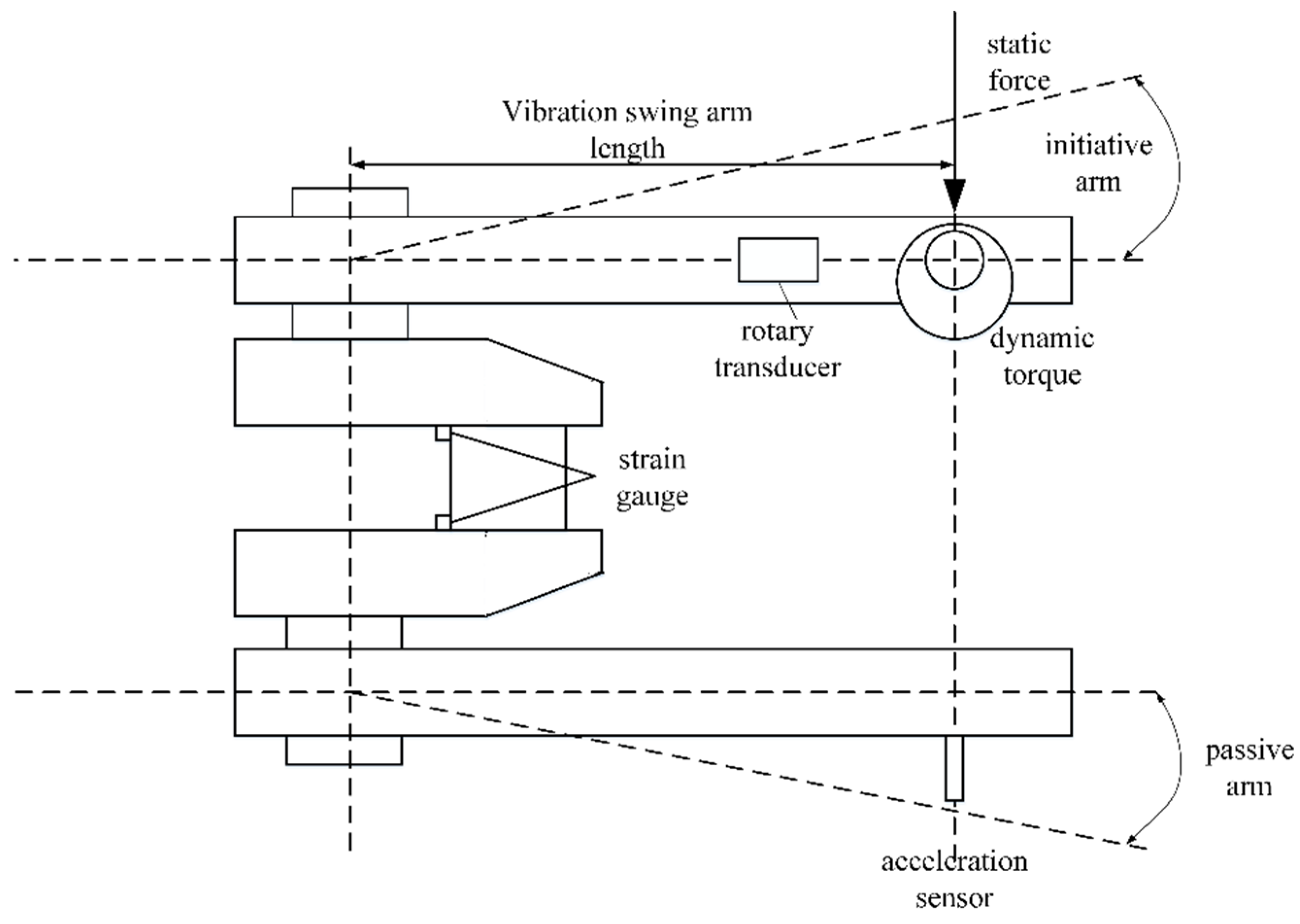
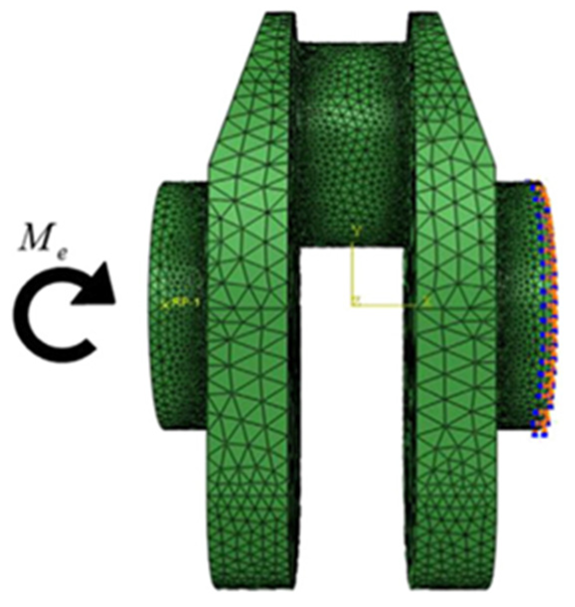
2.3. Experiment Verification Method

In order to check the accuracy of the predictions based on the method proposed by this paper, it is necessary to carry out professional experiment. Figure 1 shows the structural features of this equipment, from which it can be discovered that one of the crankpins is firmly clamped by two arms. During the experiment process, a cyclic load generated by the electromotor is applied on the master arm of the equipment. Due to the resonance effect of the equipment, an amplifying cyclic bending load will be generated and applied on the crankpin. As the experiment lasts, fatigue crack will occur at the fillet of the crankpin and result in the reduction in the value of the system natural frequency. In order to avoid the increase in the responsive acceleration, the rotate speed of the electromotor should be adjusted accordingly. When the decrement of the speed has reached 60 rpm, the crankshaft is considered to be broken [24,25].

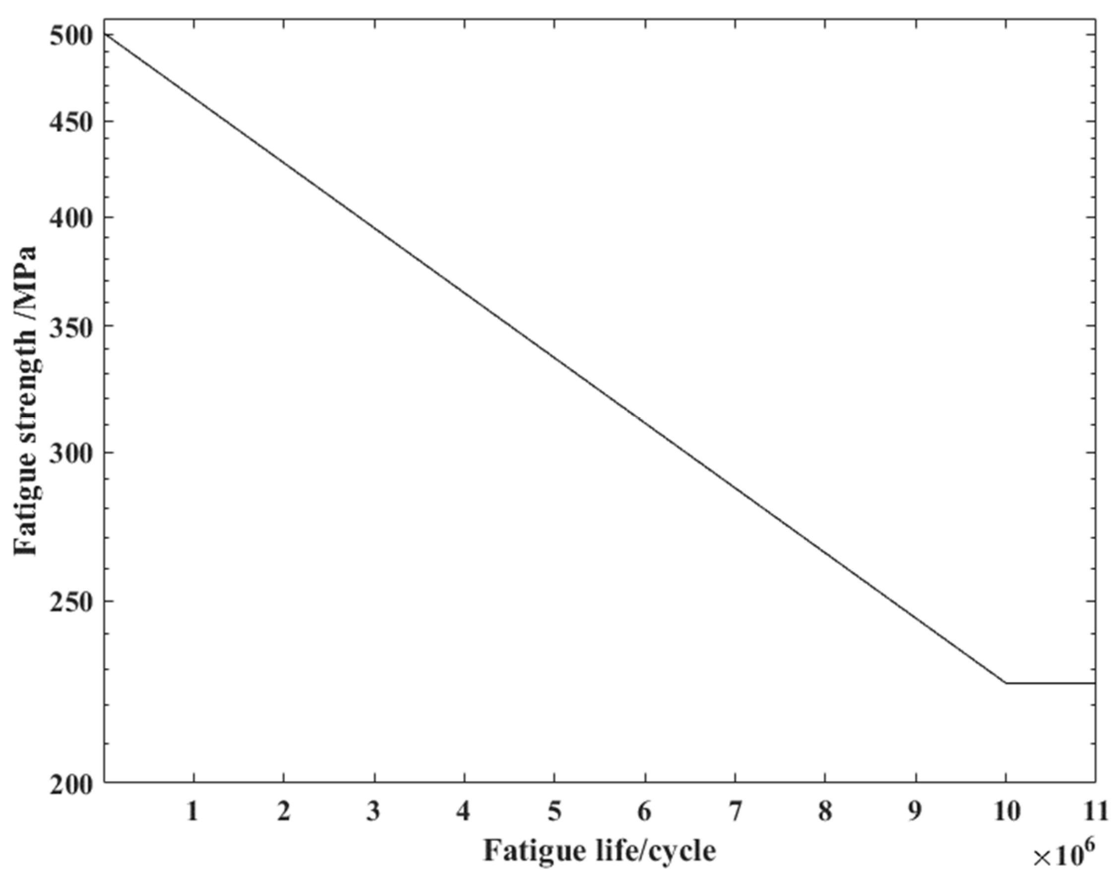
2.4. Fatigue Model Selection

As mentioned in the previous chapter, the fatigue property prediction must be proposed on a selected multi-axial fatigue damage model. At present, various multi-axial fatigue models have been applied in researching these problems. Up to now, most of the models are built based on the normal and shear stress on a preliminary defined critical plane. The definition of these models can be expressed as [26,27]:

$${\sigma }_{eq}={\tau }_{\max }+\lambda {\sigma }_{n\max }$$

(3)

As shown in equation, ${\sigma }_{n\max }$ is the maximum normal stress in the critical plane, ${\tau }_{\max }$ is the maximum shear stress in the same plane, $\lambda$ can be considered as material constant or determined by the stress condition. Based on this assumption, several experts proposed corresponding multi-axial fatigue damage models in researching different kinds of fatigue damage problems. In this paper, the type of the alternating load applied on the crankshaft is bending moment. According to previous study, the fatigue damage type of the crankshaft in this condition is shear fatigue damage. After overall consideration of the theoretical information above, a new equivalent stress model is proposed in this paper. The definition of this model can be expressed as:

$${\sigma }_{eq}=\sqrt{{\tau }_{\max }^2+\frac{1}{3}{\sigma }_{{}_{n\max }}^2}$$

(4)

As shown in Equation (5), the parameters are the same with those in Equation (2). The definition of the critical plane is the plane with the maximum shear stress. The direction of the critical plane and stress can be determined by a coordinate transform method [28]. The process of this approach is shown in Figure 2.

3. Results

3.1. Prediction of Crankshaft N0

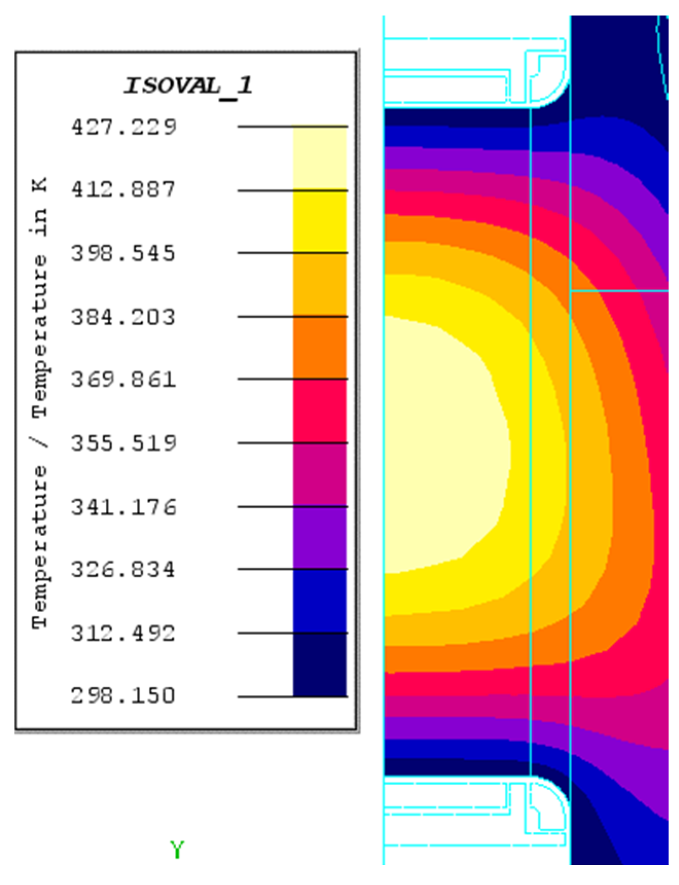
3.1.1. The Magnetic–Thermal Coupling Analysis

According to the analysis in the previous chapter, the first step is to carry out the numerical simulation of the multi-physics coupling phenomenon during the quenching process. Figure 3 shows the mesh model for the magnetic–thermal coupling analysis, from which it can be found that the whole model is composed by two parts: the quarter model of the crankpin and the far field around it. In this way, the electromagnetic field dissipation effect can be taken into consideration. In addition, the symmetry plane of the crankpin is set to be adiabatic due to the structural features of the crankpin. In order to take the accuracy and efficiency demands into account, more elements with relatively smaller sizes have been created on the surface of the crankpin area, which will be the important research object in further study. The whole model contains 207,423 elements, among which 61,376 elements belongs to the crankpin.

During the heating stage, the whole crankshaft is placed in the air. As a result of this, convective and radiative heat transfer happens between the surface of the steel part and air. According to previous study, the boundary condition in this condition can be expressed as:

$$-\lambda \frac{\partial T}{\partial n}=h(T_S-T_f)$$

(5)

As shown in this equation, h is the equivalent heat transfer coefficient, λ is the thermal conductivity, T_S is the temperature of the steel crankshaft surface and T_f is the temperature of the air. For the convective heat transfer, the value of the transfer coefficient is 100 W/(m²∙°C) in this stage. Meanwhile, for the radiative heat transfer, the value is 0.8.

In this paper, the load during the heating stage is just the high frequency alternating current inside the coils. As shown in Table 2, the values of the heating time inside different coils are not the same. For the fillet coil, the current lasts 9 s throughout the whole process. For the crankpin coil, the current works for 1 s every 3 s. Based on this stair heating approach, a generally even temperature field can be achieved at the surface of the crankpin; the results are shown in Figure 4 and Figure 5.

As shown in Figure 4, at the beginning of the heating stage, the heating depth of the crankpin is obviously shallower than that of the fillet. This phenomenon can be explained by the longer heating time and larger current density in the former area. As time passes, the difference between the values of the heating depth at different areas gradually goes down. In other words, a generally smooth temperature field has been created at the surface of the crankshaft. In addition, the surface temperature has already reached the austenite transformation point after 5 s. As a result of this, a smooth surface austenite layer can be created after cooling, which is to the benefit of the wear-resistant design of the part. After 9 s, the temperature of almost the whole crankpin has raised obviously. The surface temperature has reached 1372 K. The location of the highest temperature point is at the connecting area between the fillet and the crankpin.

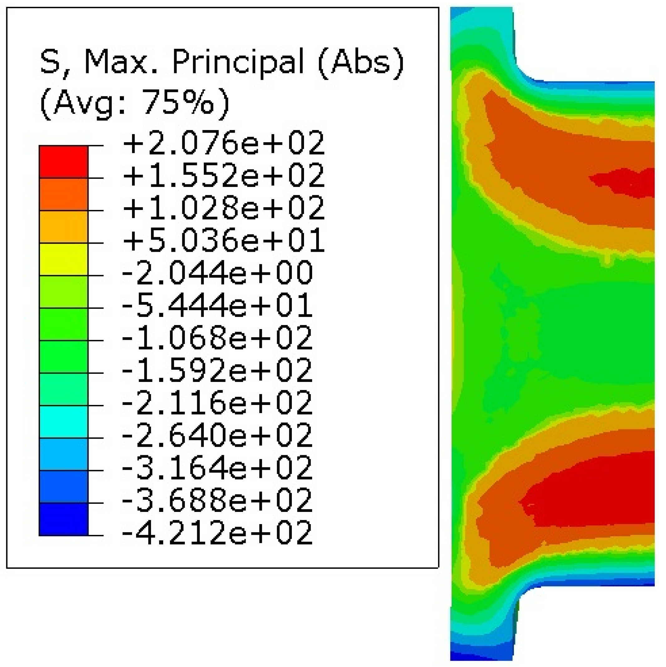
3.1.2. The Thermal-Mechanical Coupling Analysis

According to the production standard, the crankshaft should be cooled down quickly after heating. In this cooling stage, liquid coolant is sprayed to the surface of the crankpin. The whole process lasts about 10 s. As a result of this, the surface temperature drops down quickly and the temperature of the inner parts of the crankshaft begins to rise. In this way, different types of residual stress will be created at different areas of the crankpin. Figure 6 shows the temperature field after cooling, from which it can be discovered that the value of the highest temperature is 427 K, which is obviously smaller than that during the heating stage. The reason can be explained by the higher conductivity transfer coefficient in this stage. Compared with the heating stage, the value of the conductivity transfer coefficient in this stage is much larger (15,000 W/(m²∙°C)). In addition, the location of the maximum temperature point has moved to the central part of the crankshaft from the surface area.

After the liquid cooling, the crankshaft will be placed in the air for no less than 6 h. In this way, the whole crankshaft can be completely cooled. During these 6 h, the evolution process of the temperature field will result in the changing thermal stress field throughout the whole process, which will finally transfer to the residual stress field after being completely cooled. In other words, the load that creates the residual stress field is just the evolution process of the temperature field in this stage. The finite element model in Figure 7 is just selected to carry out the thermal-mechanical coupling numerical simulation in this stage. As shown in this figure, both the anterior-posterior and right-and-left planes of symmetry are fixed. The whole model is generated based on the platform of the software Abaqus 6.14, which contains 34,062 elements and 56,234 nodes. The type of the element in this stage is C3D10.

Based on this model, the residual stress field of the crankshaft after quenching can be proposed. The result is shown in Figure 8.

As shown in Figure 8, the maximum value of the residual stress is 734.7 MPa, which locates at the connecting area between the crankpin and the fillet. The type of residual stress at this point is compressive. While for the inner part of the crankshaft, the type of residual stress at this area is tensile.

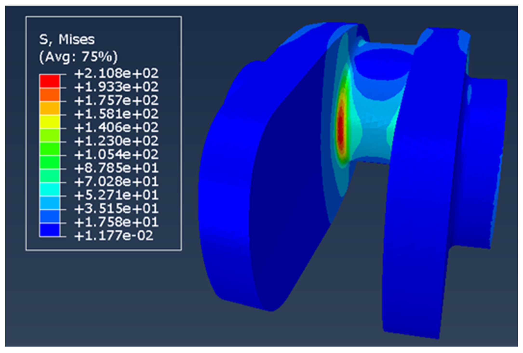
3.1.3. Equivalent Stress and Prediction Results

In this paper, the crankshaft is made of high strength alloy steel 42CrMo, the shear S-N curve of this material from the fatigue analysis software Femfat 5.2 is shown in Figure 9.

Based on the residual stress field obtained in the previous chapter, the equivalent stress of the crankshaft under a given alternating bending moment can be proposed. Figure 10 shows the finite element model for the bending fatigue analysis, from which it can be found that the right face of the crankshaft is fixed to provide the corresponding displacement boundary condition, and a bending moment is applied on the left side. The type of the element in this stage is the same with that in the residual stress field analysis stage.

Based on this 3D finite element, the stress distribution analysis of this crankshaft under a given bending moment (1000 N·m) can be realized; the result is shown in Figure 11.

As shown in Figure 11, in this stage, the fillet of the crankpin is the maximum stress point location of the crankshaft, which is the same with the bending fatigue fracture point of the crankshaft.

Table 3. Components of the stress sensor of crankshaft N0 from different sources.

Parameter	Residual Stress Field	Given Load
S11	−72.5 MPa	41.75 MPa
S22	−75.1 MPa	73 MPa
S33	−323.8 MPa	72.5 MPa
S12	75.4 MPa	−0.014 MPa
S13	−1.6 MPa	0.14 MPa
S23	2.03 MPa	74.1 MPa
Shear stress	−24.4 MPa	76.2 MPa
Normal stress	−157.3 MPa	72.4 MPa

shows the main components of the stress tensor at this point from different sources, according to our previous study, the coordinate transform method can find out the direction of the critical plane. Based on this method, the stress components of the plane from different sources are also shown in Table 3.

As a result of this, the equivalent stress of the crankshaft under a given bending moment X can be expressed as:

$${\sigma }_{eq}=\sqrt{{\left(76.2\times \frac{X}{1000}-24.4\right)}^2+\frac{1}{3}{\left(72.4\times \frac{X}{1000}-157.3\right)}^2}$$

(6)

Based on these parameters, the equivalent stress of the crankshaft under a given bending moment can be determined, as well as the fatigue life under this load. The relationship between the load and fatigue life of this crankshaft is show in Figure 12.

3.2. Prediction of Crankshaft N1

3.2.1. The Magnetic–Thermal Coupling Analysis

In order to check the universality of the model proposed in this paper, another type of quenched crankshaft made by the same material is also selected to be the object of study. Figure 13 shows the similar 3D finite element model for the magnetic–thermal coupling analysis of crankshaft N1, which contains 215,846 elements. The boundary condition is this case is just the same with that in the N0 case.

Based on this mesh model and the load information in Table 2, the magnetic–thermal coupling process analysis of this crankshaft can be carried out conveniently. The results are shown in Figure 14 and Figure 15.

As shown in Figure 14, at the beginning of this heating up stage, the heating range of the crankshaft is relatively small, mainly around the fillet of the crankpin. On the other hand, the depth of the temperature field is also smoothly located around the surface of the crankpin, which shows similar properties with that of crankshaft N0. After 12 s, the temperature of almost the whole crankpin has raised obviously. The surface temperature has reached 1285 K. The location of the highest temperature point is at the connecting area between the fillet and the crankpin.

3.2.2. The Thermal-Mechanical Coupling Analysis

In this stage, the same liquid coolant is sprayed onto the surface of the crankshaft. Figure 16 and Figure 17 shows the temperature field and the residual stress field after cooling, respectively. From these two figures, it can be discovered that after liquid cooling, the surface temperature has already dropped to room temperature, and the inner temperature has increased to 412 K. The maximum residual stress of the crankshaft after cooling is 634 MPa.

3.2.3. Equivalent Stress and Prediction Results

By repeating the finite element analysis in Figure 10, the stress tensor of this crankshaft from different load sources can be computed. The results are shown in

Table 4. Components of the stress sensor of crankshaft N1 from different sources.

Parameter	Residual Stress Field	Given Load
S11	−239.4 MPa	35 MPa
S22	−251.4 MPa	62 MPa
S33	−367.3 MPa	62.5 MPa
S12	248.7 MPa	−0.08 MPa
S13	2 MPa	0.128 MPa
S23	1.2 MPa	64.2 MPa
Shear stress	−64.4 MPa	64 MPa
Normal stress	−363.3 MPa	62.4 MPa

.

As a result of this, the equivalent stress of the crankshaft under a given bending moment X can be expressed as:

$${\sigma }_{eq}=\sqrt{{\left(64\times \frac{X}{1000}-64.4\right)}^2+\frac{1}{3}{\left(62.4\times \frac{X}{1000}-363.2\right)}^2}$$

(7)

Based on this equation, the equivalent stress of the crankshaft under a given bending moment can be determined, as well as the fatigue life under this load. The relationship between the load and fatigue life of this crankshaft is shown in Figure 18.

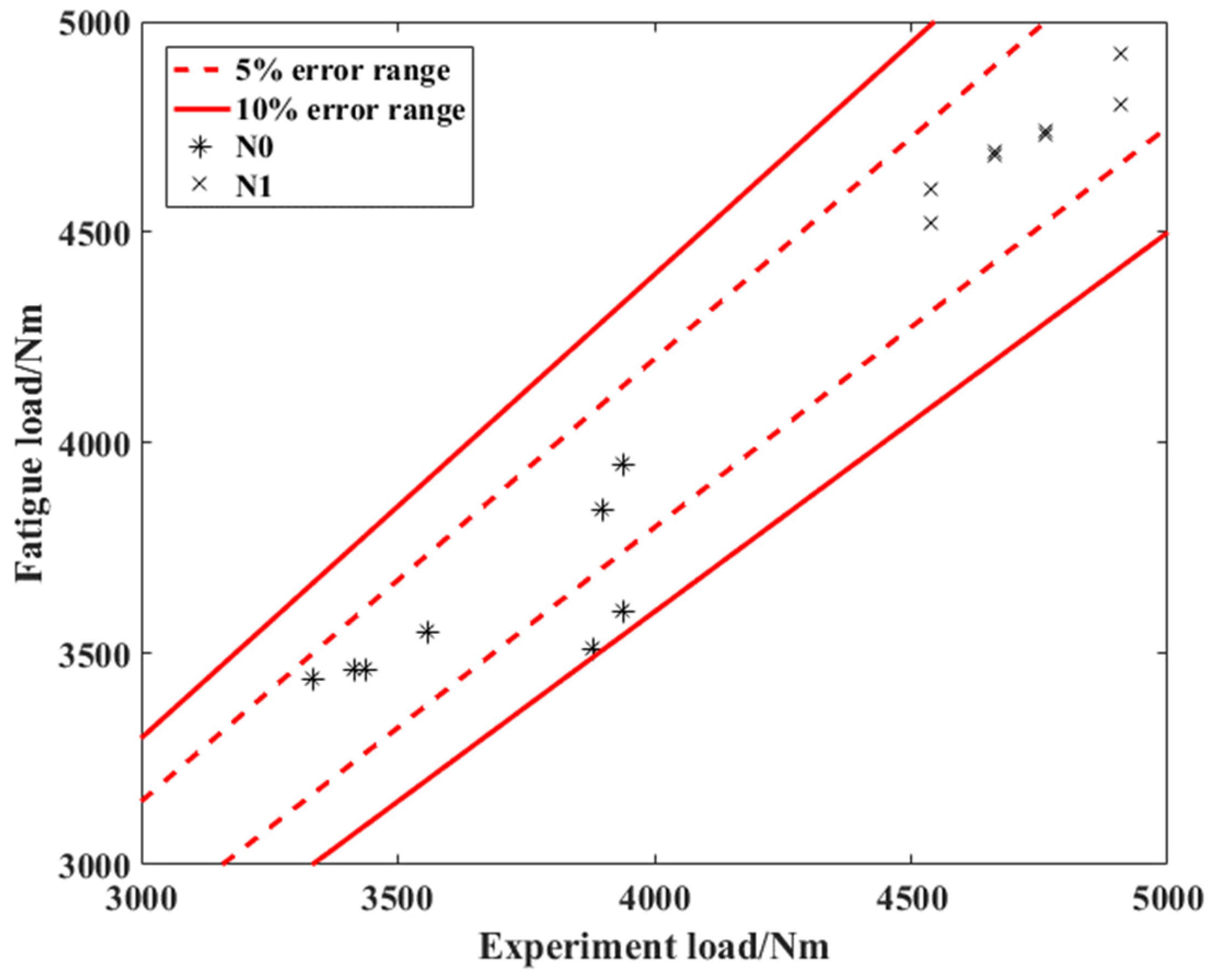
4. Experimental Verification and Discussion

In order to check the accuracy of the predictions, corresponding experimental verification is necessary. According to previous study, for engine parts such as the crankshaft, the accuracy of the fatigue property prediction can usually be evaluated by three factors: the location of the fatigue fracture range, the fatigue limit load under the 50% survival rate, and the fatigue distribution property (usually by comparing the predicted fatigue life under a given load and the actual experiment data, or the predicted fatigue load under a specified fatigue life and the actual fatigue load). For the crankshaft, the fatigue fracture crack usually initiates from the fillet of the crankpin, which is in agreement with the maximum stress point in Figure 12. So, the comprehensive verification can be conducted by the latter two factors.

Table 5. Fatigue experimental results of crankshaft N0.

Load Value/N·m	Load Cycle
3335	6,711,179
3436	6,187,261
3881	4,502,460
3941	2,465,780
3941	273,493
3901	548,588
3416	6,142,771
3557	3,509,554

and

Table 6. Fatigue experimental results of crankshaft N1.

Load Value/N·m	Load Cycle
4909	496,300
4909	252,286
4664	868,306
4664	901,425
4764	687,944
4764	652,265
4541	1,435,103
4541	2,221,044

show the bending fatigue results of both crankshafts. According to the modified SAFL method (statistical analysis for fatigue limit), the values of the fatigue limit load of these two crankshafts under the 50% survival rate are 3335 N·m and 4345 N·m, respectively. By comparing these two parameters with the prediction from Equations (5) and (6), a clear conclusion can be proposed that the accuracy of the predictions in both cases are high enough for engineering applications (the relative errors are less than 5% in both cases).

In actual engineering application, the service life of a crankshaft is limited to a certain number of cycles depending on the demand of the travelling distance. As a result of this, compared with the common fatigue property evaluation parameter (usually the fatigue life under a given load) [29,30], it is more important to correctly evaluate the high-cycle fatigue load of a crankshaft under a specified fatigue life [31,32,33,34]. Figure 19 shows the distribution property of the fatigue life of both crankshafts, from which it can be found that most of the predictions are located within the double error range: only a few points are located between the double and triple times error ranges. After a general consideration based on the three factors, it is well-founded to say that this method can provide high enough accuracy in predicting the fatigue property of both types of steel crankshafts; thus, it can be considered to be applied in guiding the design and manufacturing process of the part.

According to our previous study, the damage type of the crankshaft in this condition is shear fatigue damage. Compared with the formal multi-axial fatigue damage models, the model proposed by this paper can predict the fatigue property of two types of steel crankshaft produced according to different technological parameters. However, these two types of crankshafts were produced by the same material 42CrMo, so more work should be conducted in researching the feasibility of this method in predicting the fatigue property of the crankshafts made by other materials.

5. Conclusions

In this paper, the fatigue property prediction method of the quenched steel crankshaft was selected to be the object of study. First, the whole manufacturing process was simulated by the multi-physics field coupling analysis, then the fatigue property of two types of steel crankshafts was predicted based on the combination of the residual stress obtained in the previous step, and a new multi-axial fatigue damage model proposed in this paper. Finally comprehensive experimental verification was conducted by three main factors of the prediction. The main conclusions of the research are shown as followed:

(1)

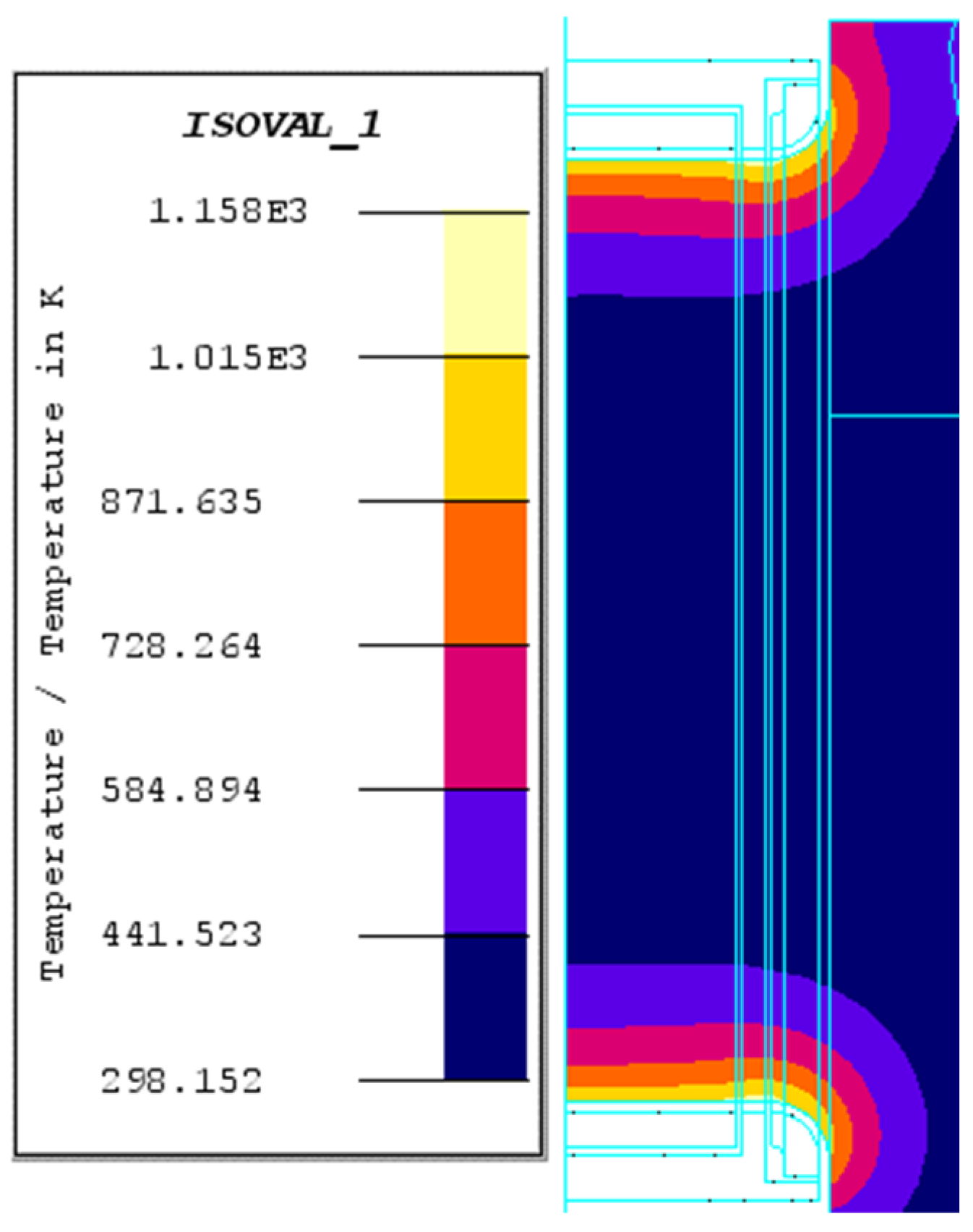
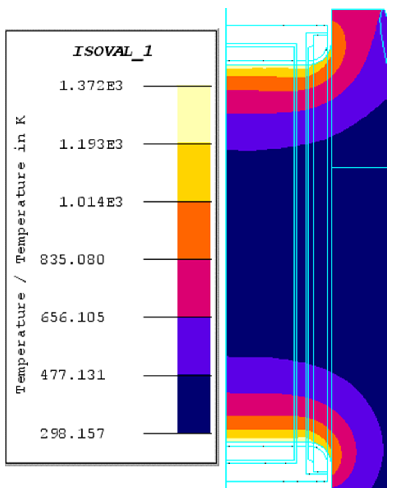
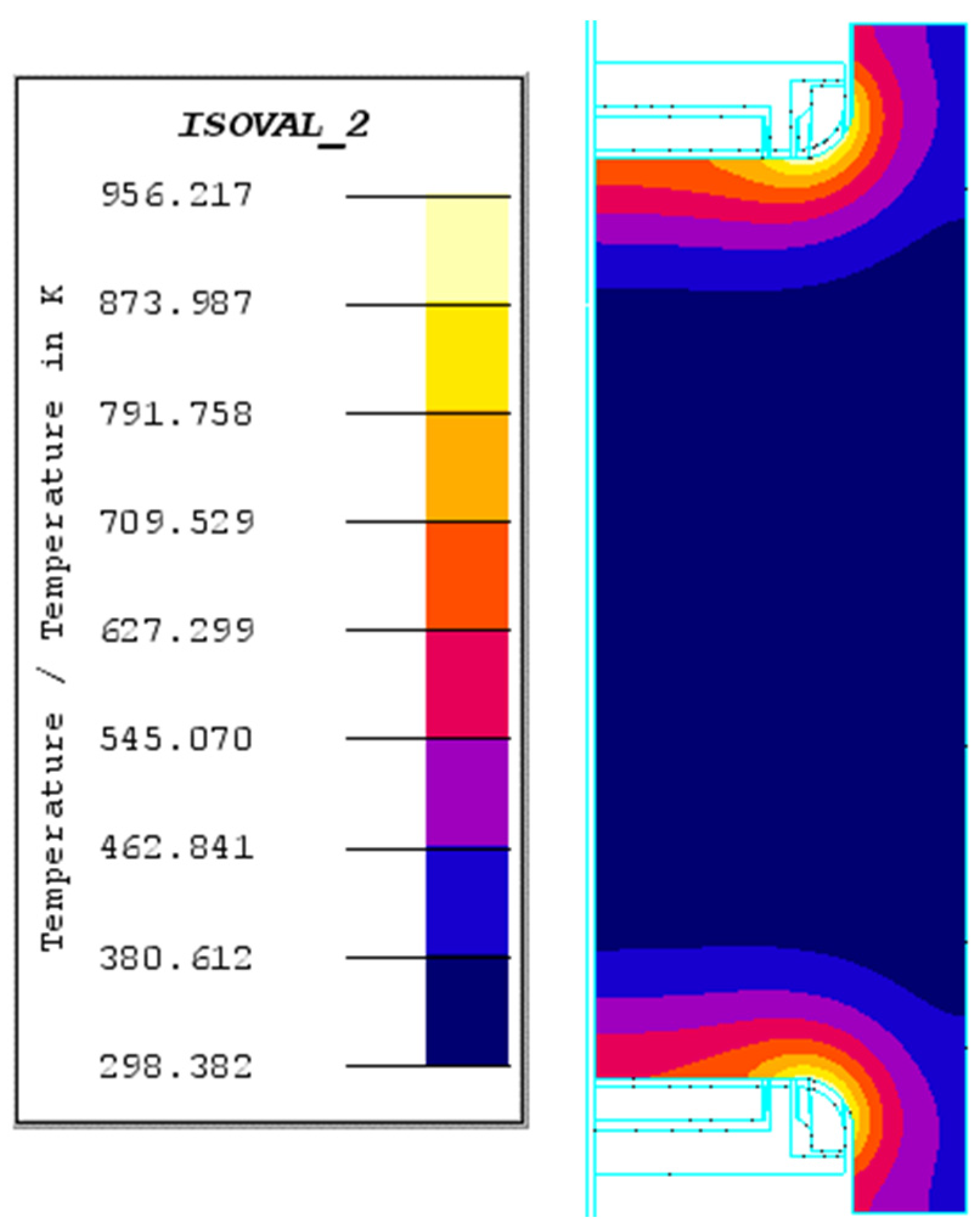
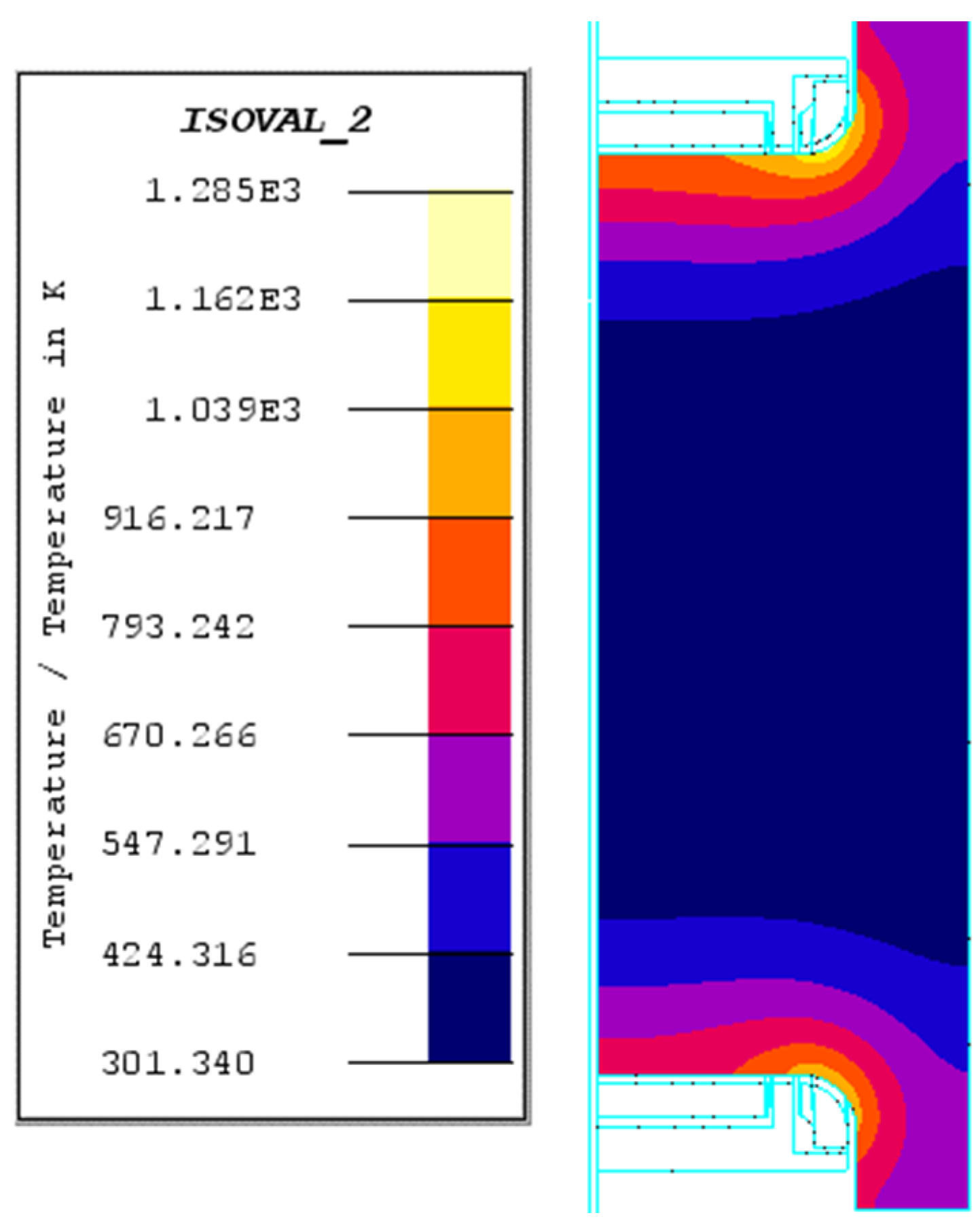
For both crankshafts, during the heating up stage, the temperature at the fillet increased more quickly than that at the crankpin surface, which could be attributed to the longer effective heating time of the former. In addition, the uniform temperature fields at the surface of the crankpin area is useful to form the uniform layer.

(2)

After liquid cooling, the temperature of the surface dropped rapidly, and the internal body of the crankshaft began to rise. Additionally, the compressive residual stress was generated at the surface and the tensile residual stress was created within the central area.

(3)

The multi-axial fatigue damage model proposed in this paper can accurately predict the fatigue property of no less than one type of steel crankshaft, which makes it useful to be applied in guiding the design and manufacturing process of the part.

References

1. Jie, T.; Tong, J.; Shi, L. Differential steering control of four-wheel independent-drive electric vehicles. Energies 2018, 11, 2892. [Google Scholar]
2. Tian, J.; Wang, Q.; Ding, J.; Wang, Y.; Ma, Z. Integrated Control With DYC and DSS for 4WID Electric Vehicles. IEEE Access 2019, 7, 124077–124086. [Google Scholar] [CrossRef]
3. Lin, Y.; Xiao, M.H.; Liu, H.J.; Li, Z.L.; Zhou, S.; Xu, X.M.; Wang, D.C. Gear fault diagnosis based on CS-improved variational mode decomposition and probabilistic neural network. Measurement 2022, 192, 110913. [Google Scholar] [CrossRef]
4. Xu, X.; Zhang, L.; Jiang, Y.; Chen, N. Active control on path following and lateral stability for truck–trailer com-binations. Arab. J. Sci. Eng. 2019, 44, 1365–1377. [Google Scholar] [CrossRef]
5. Xu, X.; Lin, P. Parameter identification of sound absorption model of porous materials based on modified particle swarm optimization algorithm. PLoS ONE 2021, 16, e0250950. [Google Scholar] [CrossRef]
6. Xu, X.; Chen, N.; Zhang, L.; Chen, N. Hopf Bifurcation Characteristics of the Vehicle with Rear Axle Compliance Steering. Shock Vib. 2019, 2019, 3402084. [Google Scholar] [CrossRef] [Green Version]
7. Jiri, P.; Zdenek, P.; David, D. Service behavior of nitride layers of steels for military applications. Coating 2020, 10, 975. [Google Scholar]
8. Sackl, S.; Leitner, H.; Zuber, M.; Clemens, H.; Primig, S. Induction Hardening vs Conventional Hardening of a Heat Treatable Steel. Met. Mater. Trans. A 2014, 45, 5657–5666. [Google Scholar] [CrossRef]
9. Prisco, U. Case microstructure in induction surface hardening of steels: An overview. Int. J. Adv. Manuf. Technol. 2018, 98, 2619–2637. [Google Scholar] [CrossRef]
10. Qi, P.; Sun, Q.; Zhong, J.; Wang, G.; Liu, X.; Liu, W. Effects of electromagnetic induction hardening on the microstructure and mechanical properties of B1500HS steel. IOP Conf. Ser. Mater. Sci. Eng. 2020, 892, 012017. [Google Scholar] [CrossRef]
11. Barglik, J. Induction contour hardening of gear wheels made of steel 300M. IOP Conf. Ser. Mater. Sci. Eng. 2018, 424, 012062. [Google Scholar] [CrossRef]
12. Barglik, J.; Smagór, A.; Smalcerz, A. Induction hardening of gear wheels of steel 41Cr4. Int. J. Appl. Electromagn. Mech. 2018, 57, 3–12. [Google Scholar] [CrossRef]
13. Torres, H.; Pérez-González, F.A.; Zapata-Hernández, O.; Garza-Montes-deOca, N.F.; Ramírez-Ramírez, J.H.; Fried, Z.; Felde, I.; Réger, M.; Colás, R. Modeling the Induction Hardening of High-Carbon Saw Blades Reference. Mater. Perform. Charact. 2019, 8, 261–271. [Google Scholar]
14. Baldan, M.; Stolte, M.H.; Nacke, B.; Nürnberger, F. Improving the Accuracy of FE Simulations of Induction Tempering Toward a Micro-structure-Dependent Electromagnetic Model. IEEE Trans. Magn. 2020, 56, 1–9. [Google Scholar] [CrossRef]
15. Tong, D.; Gu, J.; Yang, F. Numerical simulation on induction heat treatment process of a shaft part: Involving induction hardening and tempering. J. Mater. Process. Technol. 2018, 262, 277–289. [Google Scholar] [CrossRef]
16. Tong, D.; Gu, J.; Totten, G.E. Numerical investigation of asynchronous dual-frequency induction hardening of spur gear. Int. J. Mech. Sci. 2018, 142, 1–9. [Google Scholar] [CrossRef]
17. Fisk, M.; Lindgren, L.E.; Datchary, W.; Deshmukh, V. Modelling of induction hardening in low alloy steels. Finite Elem. Anal. Des. 2018, 144, 61–75. [Google Scholar] [CrossRef]
18. Wu, C.; Sun, S. Crankshaft High Cycle Bending Fatigue Research Based on a 2D Simplified Model and Different Mean Stress Models. J. Fail. Anal. Prev. 2021, 21, 1396–1402. [Google Scholar] [CrossRef]
19. Sun, S.S.; Zhang, X.; Wu, C.; Wan, M.; Zhao, F. Crankshaft high cycle bending fatigue research based on the simulation of electromagnetic induction quenching and the mean stress effect. Engl. Fail. Anal. 2021, 122, 105214. [Google Scholar]
20. Li, J. Numerical Studies on the Induction Quenching Process of Crankshaft; Beijing Institute of Technology: Beijing, China, 2015. [Google Scholar]
21. Lim, B.K. Analysis of fatigue life of SPR (self-piercing riveting) jointed various specimens using FEM. In Proceedings of the International Welding/Joining Conference-Korea, IWJC-Korea 2007; Small Business Training Institute: Ansan, Korea, 2008. [Google Scholar]
22. Hömberg, D.; Liu, Q.; Montalvo-Urquizo, J.; Nadolski, D.; Petzold, T.; Schmidt, A.; Schulz, A. Simulation of multi-frequency-induction-hardening including phase transitions and me-chanical effects. Finite Elem. Anal. Des. 2016, 121, 86–100. [Google Scholar] [CrossRef]
23. Sun, S.S.; Yu, X.-L.; Li, J.F. A study on the equivalent fatigue of crankshaft structure based on the theory of multi-axial fatigue. Automot. Eng. 2016, 38, 1001–1005. [Google Scholar]
24. Zhou, X.; Yu, X. Failure criterion in resonant bending fatigue test for crankshafts. Chin. Intern. Combust. Engine Eng. 2007, 28, 45–47. [Google Scholar]
25. Zhou, X.; Yu, X. Error analysis and load calibration technique investigation of resonant loading fatigue test for crankshaft. Trans. Chin. Soc. Agric. Mach. 2007, 4, 35–38. [Google Scholar]
26. Brown, M.W.; Miller, K.J. A theory for fatigue failure under multi-axial stress-strain conditions. Proc. Inst. Mech. Eng. 1973, 187, 1847–1982. [Google Scholar] [CrossRef]
27. Sun, S.S.; Wan, M.S.; Wang, H. Crankshaft fatigue research based on modified multi-axial fatigue model. J. Mech. Electr. Engl. 2019, 36, 797–802. [Google Scholar]
28. Sun, S.S.; Yu, X.L.; Chen, X.P.; Liu, Z.T. Component structural equivalent research based on different failure strength criterions and the theory of critical distance. Engl. Fail. Anal. 2016, 70, 31–43. [Google Scholar] [CrossRef]
29. Zhang, Y.; Wang, A. Remaining Useful Life Prediction of Rolling Bearings Using Electrostatic Monitoring Based on Two-Stage Information Fusion Stochastic Filtering. Math. Probl. Engl. 2020, 2020, 2153235. [Google Scholar] [CrossRef]
30. Wang, H.; Zheng, Y.; Yu, Y. Joint Estimation of SOC of Lithium Battery Based on Dual Kalman Filter. Processes 2021, 9, 1412. [Google Scholar] [CrossRef]
31. Wang, H.; Zheng, Y.; Yu, Y. Lithium-Ion Battery SOC Estimation Based on Adaptive Forgetting Factor Least Squares Online Identification and Unscented Kalman Filter. Mathematics 2021, 9, 1733. [Google Scholar] [CrossRef]
32. Zhou, W.; Zheng, Y.; Pan, Z.; Lu, Q. Review on the Battery Model and SOC Estimation Method. Processes 2021, 9, 1685. [Google Scholar] [CrossRef]
33. Chang, C.; Zheng, Y.; Sun, W.; Ma, Z. LPV Estimation of SOC Based on Electricity Conversion and Hysteresis Characteristic. J. Energy Engl. 2019, 145, 04019026. [Google Scholar] [CrossRef]
34. Chang, C.; Zheng, Y.; Yu, Y. Estimation for Battery State of Charge Based on Temperature Effect and Fractional Extended Kalman Filter. Energies 2020, 13, 5947. [Google Scholar] [CrossRef]
Figure 1. The structure diagram of the bending fatigue experiment equipment.
Metals 12 01296 g001
Figure 2. The working principle of the coordinate transform method.
Metals 12 01296 g002
Figure 3. A quarter-pin model in the electromagnetic field of crankshaft N0.
Metals 12 01296 g003
Figure 4. Temperature field of crankshaft N0 during the heating stage (T = 5 S).
Metals 12 01296 g004
Figure 5. Temperature field of crankshaft N0 during the heating stage (T = 9 S).
Metals 12 01296 g005
Figure 6. Temperature field of crankshaft N0 after liquid cooling.
Metals 12 01296 g006
Figure 7. Displacement boundary conditions of the crankshaft for thermal-mechanical coupling analysis.
Metals 12 01296 g007
Figure 8. The residual stress field distribution of crankshaft N0.
Metals 12 01296 g008
Figure 9. The shear S-N curve of the material.
Metals 12 01296 g009
Figure 10. The finite element model for bending analysis.
Metals 12 01296 g010
Figure 11. The stress distribution of crankshaft N0 (under the given bending moment).
Metals 12 01296 g011
Figure 12. The load-life relationship of crankshaft N0.
Metals 12 01296 g012
Figure 13. A quarter-pin model in the electromagnetic field of crankshaft N1.
Metals 12 01296 g013
Figure 14. Temperature field of crankshaft N1 during the heating stage (T = 6 S).
Metals 12 01296 g014
Figure 15. Temperature field of crankshaft N1 during the heating stage (T = 12 S).
Metals 12 01296 g015
Figure 16. Temperature field of crankshaft N1 after liquid cooling.
Metals 12 01296 g016
Figure 17. The residual stress field distribution of crankshaft N1.
Metals 12 01296 g017
Figure 18. The load-life relationship of crankshaft N1.
Metals 12 01296 g018
Figure 19. Fatigue load predictions of both crankshafts.
Metals 12 01296 g019