1. Introduction
In recent years, Additive Manufacturing (AM) processes have become increasingly commonplace due to the advantages they offer over traditional manufacturing methods. Arguably one of the most promising AM processes is that of wire-fed Electron Beam Additive Manufacturing (EBAM). This process is similar to electron beam welding and utilizes high-energy electron beams to fuse metal wires together. Similar to other forms of additive manufacturing, wire-fed EBAM allows for the printing of full-density, functional as-printed parts requiring minimal post-processing treatments [
1,
2].
Wire-fed EBAM processes have the advantage of high production speeds in addition to the ease of feedstock storage, availability and handling compared to powder-based AM. Importantly, wire-fed AM also originates from a feedstock less susceptible to contamination [
2,
3,
4,
5,
6,
7,
8]. Finally, the shape and length scale of the feedstock—mm sized diameter wire as opposed to μm sized spherical metal particles [
1,
3,
9,
10]—help to improve the density of EBAM prints and diminishes the risk for porosity and inclusions. However, as with all AM processes, there are issues of residual stresses, occasional internal voids as well as significant material property anisotropy. These are inherent to the printing processes and the thermo-mechanical interactions between layers [
3,
9,
11], however they remain some of the most pressing research frontiers for AM to become more widespread.
Generally, AM improves the “buy-to-fly” ratio—or, the mass ratio between the original stock material used to produce the part and that of the final machined part. The buy-to-fly of traditionally manufactured titanium aircraft components ranges from 12:1 to 25:1 [
12,
13]. This translates to approximately 90% of the initial material being discarded for the final print. AM not only has the potential to reduce a part’s overall life-cycle impact, it also offers engineers and designers improved design freedom to create products that are unique, manufacturable at low volumes, and economical [
2]. Williams, Martina, et al. [
14] analyzed wire-arc additive manufacturing of Ti-6Al-4V and steel printed parts, determining that depending upon the deposition rate, ranging from 1 kg/h to 4 kg/h, they could achieve a buy-to-fly ratio of less than than 1.5. At higher deposition rates the fidelity of the part is compromised and requires significant machining, deposition of larger amounts of material thus increasing the buy-to-fly ratio to be more in line with traditionally manufactured parts.
The thermo-mechanical cycles and processing parameter variability that is intrinsic to AM printing, subsequently influence all aspects of the final part’s material properties [
9,
15,
16]. Variations in thermal experiences and processing conditions result in microstructural gradients, making the science of predicting the material properties and resulting residual stresses a complex multiphysics simulation problem. One method to experimentally determine the material properties involves the use of destructive testing procedures in order to observe the microstructures associated with specific print geometries and processing parameters [
7,
17,
18,
19]. However, destructive testing is costly in both time and resources and negates the improved life-cycle benefits of AM. Ideally, a predictive model could be used instead to predict the material anisotropy based on processing conditions alone, relinquishing the need to destructively investigate each part. Such a parameter-to-property model would by-pass the need for multiscale multiphysics modeling, which remains to this day a time consuming and computationally intensive endeavor.
Processing parameters heavily influence the material properties of the final build. Specifically, heat input, energy distribution, and wire feed have all been shown to play a significant role [
5,
20]. The proper tuning of energy input and wire feed is essential to the formation and control of a stable melt pool which in turn affects the mechanical properties. As such, efforts were put forth by [
11,
21,
22] to model the effect of thermo-mechanical cycles on the evolution of the material’s localized microstructure. Chekir, Tian, et al. investigated laser wire deposited Ti-6Al-4V of heights between 40 and 65 mm by developing a finite element thermal model in order to predict thermal distributions caused by the deposition process [
11]. Their study revealed that processing conditions promoted the coarsening of microstructures due to multiple melting-solidification cycles. The group also investigated the effect of post-processing treatments upon the material grains, concluding that annealing or a hot isostatic pressing followed by aging preserves prior
grain morphology with coarsening of the microstructure. Similarly, Sikan, Wanjara, et al. [
21] developed a 3D transient, fully coupled thermo-mechanical finite element model that accurately predicted the cooling rates, grain morphology and microstructure of EBAM printed Ti-6Al-4V. The model, when validated against experimental results, had thermal predictions with an average error of 3.7% [
21]. Bonifaz and Watanabe examined the micro residual stresses and micro plastic strains in SAE-AISI-1524 gas tungsten arc welded joints. The model uses a transient, non-linear multiscale finite element approach [
22] that incorporates anisotropy through the use of the maximum and minimum Young’s modulus in the stiffest and least stiff directions, respectively. These studies demonstrate that by using high resolution, high powered computational modeling it is possible to analyze the melt pool, microstructure and stresses for both as printed and post-processed parts. While these time intensive models are useful, a real-time estimate of the material properties during print would provide the possibility of on-the-fly adjustments to maintain bounds of the material properties.
Given the complexity in predicting the material properties resulting from layer-by-layer printing processes, there has been a shift towards the utilization of Neural Networks (NN), genetic algorithms and other Machine learning approaches to modeling at large [
23]. These methods are informed by the physics of the process, but use more direct models that, for specific geometries and builds, can be trained to predict material properties from microstructure [
24] or even from the build’s processing parameters alone. Statistical models [
24,
25] or machine learning methods that make use of long short-term memory (LSTM) networks [
26] or other machine learning architectures [
23,
27] in order to improve prediction models. NNs are useful as they can provide accurate predictions of the printed metal tensile strength by utilizing LSTM architecture, and in situ data or process parameters—such as thermal data, printing speed, and layer height [
26]. It is important to note, however, that NNs and hybrid NNs do require a degree of caution due to their tendency to overfit solutions. Additionally, they remain restricted to specific print geometries related to the training data supplied.
Predictive models based on processing parameters alone, such as this one and those by Zhang, Wang, and Gao [
26], Weglowski et al. [
7] and others that have been previously discussed, bypass the need for destructive testing, saving money and time. However, key processing parameters can vary between the different types of AM and must be incorporated into the models. Yao, Zhou, and Huang [
28] analyzed the double-pulsed gas metal arc welding (DP-GMAW) and provided a framework to determine influential process parameters for double-pulsed gas metal arc welding (DP-GMAW). Utilizing their framework, they were able to determine the optimal processing parameters needed to generate optimal weld beads for prints. Their work showed that the most influential factors for welding quality were the welding speed, followed by twin pulse frequency and twin pulse current. Carefully controlling these processing conditions, can lead to more efficient printing, consistent builds and minimizing the need for destructive testing.
The main aim of the current study is to provide the methodology needed to determine the yield and ultimate tensile strengths of Ti-6Al-4V printed parts as a function of the process variables at any given location within the build. The paper is structured as follows:
Section 2 presents the materials, printing process, and linear regression model methods used to predict yield and ultimate tensile strengths.
Section 3 provides an overview and discussion of the predicted results. Finally, a summary of the work is given along with a discussion of the future direction of the project.
4. Discussion
The linear predictive model is able to predict the and of as printed EBAM parts. The model was processing condition dependent, i.e., changed with each NP’s processing conditions.
It was shown that by including the cooling rate term in the linear regression model showed an increased accuracy of the model’s ability to predict the vertical and by and , respectively, while the horizontal values were improved by and , respectively. Further, by including the volume variable to represent the surrounding heat sink in the linear regression model improved the accuracy of the predicted vertical and by and , respectively, while the horizontal values were improved by and , respectively.
The coefficients of the linear regression model also confirm the interconnection of the processing variables to one another. For instance, if is modulated there will be a subsequent change in the interpass temperature which is represented by the cooling rate. Therefore, there will be a variation in the coefficients of the model between successive printings unless the bulk majority of the processing variables remain constant between prints. The model’s coefficients also provides insight into the relevancy of the processing variables to predicting the material strength; variables with small coefficients, i.e., with magnitudes of less than 10, are nearly insignificant for predicting material strength when compared with other processing variables that relate directly to thermal history.
As mentioned previously, the printed geometry was chosen to help simulate a wide range of possible print geometries expected to be printed in industry. The medley of geometries within the print should allow the linear regression model to be suitable for other print geometries and sizes than the ones presented in this study.
The linear regression model improved as build conditions improved, creating a more reliable—or consistent—EBAM print. Some dependencies and tendency to overfitting due to the number of test samples that are included. NP1, predictably, had the worst predictive results due to the distortion of the build, of the test build while NP2 and NP3 produced linear models that more accurately predicted the and for both horizontally and vertically oriented test pieces. However, for both NP2 and NP3 the linear regression model had a significantly higher degree of accuracy when predicting the strengths of horizontally oriented test pieces when compared to their vertically oriented counterparts.
The discrepancy in prediction ability could be explained from the need to improve the model’s ability to predict the cooling rate, or ideally monitor the cooling rate in situ. Presently, the model approximates the cooling rate at a point in the build based upon the amount of time the machine has been running and then takes the average of it. This approximation might oversimplify the complex thermal interactions in the vertical build direction and, subsequently, not accurately represent the cooling rate’s influence upon the final material properties. Similarly, when comparing the weights of each of the terms of the linear model, the volume term has significantly more influence upon the predicted strength in the vertical orientation than in the horizontal. Thus, an examination of the volume might be necessary to further improve the model.
NP3 has the largest number of samples tested for the horizontal direction, while NP2 has the largest number of tested samples in the vertical direction with 43 and 34 samples, respectively. Generally, with the exception of the vertical prediction for NP3, the value increases with a decreased number of samples. Therefore, it may be necessary to determine if the linear regression model is overfitting specific data points and put forth further analysis into outliers, or other inconsistencies, in the data that might otherwise skew the results.
Furthermore, it was also shown that the beadwidth and energy density generally stayed within the same order of magnitude between prints. The values also remained in the same order of magnitude regardless of the orientation of the specimen. The general consistency across all of the test runs confirms the importance that beadwidth and energy density have in creating a reliable, consistent print. Similarly, it confirms the necessity of including and processing variables for accurate material property prediction.
Author Contributions
Methodology, validation, and formal analysis, C.V.H.; investigation of range of value analysis, A.P.; data curation, further validation, original draft preparation, review and editing, T.J.; supervision, project administration, and funding acquisition, D.G.H. All authors have read and agreed to the published version of the manuscript.
Funding
This material is based upon work supported by the Defense Advanced Research Projects Agency under Contract No. HR0011-12-C-0035 (“An Open Manufacturing Environment for Titanium Fabrication”). The views, opinions and/or findings expressed are those of the authors and should not be interpreted as representing the official views or policies of the Department of Defense or the U.S. Government.
Acknowledgments
The authors would like to acknowledge the support and collaborations that made this work possible. Thank you to Scott Stecker at Sciacky, Inc. for the data and discussions about improving the processing conditions for AM printing. Thank you to Peter Collins from Iowa State University, whose communications and knowledge inspired this work. Thank you to DARPA for the funding which made this research possible. Thank you to Julian Booream for his contribution to the solidworks model.
Conflicts of Interest
The authors declare no conflict of interest.
Abbreviations
The following abbreviations and nomenclature are used in this manuscript:
| AM | Additive Manufacturing |
| EBAM | Electron Beam Additive Manufacturing |
| NN | Neural Network |
| LSTM | Long short-term memory |
| DP-GMAW | Double-pulsed Gas Metal Arc Welding |
| NP | Notional Part |
| HTX | Heat Treatment |
| NDE | Non-destructive evaluation |
| Ultimate Tensile Strength |
| Yield Strength |
| Bead width |
| Accelerating voltage |
| Beam current |
| Beam focus |
| Chamber vacuum level |
| Wire feed reference speed |
| Deposition nozzle speed |
| Vertical height above the deposition plate |
| Energy density |
| Cooling rate |
| Volume below current print location |
| t | Time at deposition for the specimen |
| Time at bead initiation |
| Average vertical height for the specimen |
| Correlation coefficient |
| Specimen’s current print location in the X |
| Specimen’s current print location in the Y |
| Specimen’s current print location in the Z |
References
- Gong, X.; Anderson, T.; Chou, K. Review on powder-based electron beam additive manufacturing Technology. In International Symposium on Flexible Automation; American Society of Mechanical Engineers: Les Ulis, France, 2014. [Google Scholar]
- Bikas, H.; Stavropoulos, P.; Chryssolouris, G. Additive manufacturing methods and modeling approaches: A critical review. Int. J. Adv. Manuf. Technol. 2016, 83, 389–405. [Google Scholar] [CrossRef] [Green Version]
- Pushilina, N.; Stepanova, E.; Stepanov, A.; Syrtanov, M. Surface modification of the ebm ti-6al-4v alloy by pulsed ion beam. Metals 2021, 11, 512. [Google Scholar] [CrossRef]
- Brandl, E.; Palm, F.; Michailov, V.; Viehweger, B.; Leyens, C. Mechanical properties of additive manufactured titanium (Ti-6Al-4V) blocks deposited by a solid-state laser and wire. Mater. Des. 2011, 32, 4665–4675. [Google Scholar] [CrossRef]
- Zhao, J.; Zhang, B.; Li, X.; Li, R. Effects of metal-vapor jet force on the physical behavior of melting wire transfer in electron beam additive manufacturing. J. Mater. Process. Technol. 2015, 220, 243–250. [Google Scholar] [CrossRef]
- Rodrigues, T.A.; Duarte, V.; Miranda, R.M.; Santos, T.G.; Oliveira, J.P. Current status and perspectives on wire and arc additive manufacturing (WAAM). Materials 2019, 12, 1121. [Google Scholar] [CrossRef] [Green Version]
- Weglowski, M.S.; Błacha, S.; Pilarczyk, J.; Dutkiewicz, J.; Rogal, L. Electron beam additive manufacturing with wire—Analysis of the process. In AIP Conference Proceedings; American Institute of Physics Inc.: Melville, NY, USA, 2018; Volume 1960. [Google Scholar] [CrossRef]
- Negi, S.; Nambolan, A.A.; Kapil, S.; Joshi, P.S.; Manivannan, R.; Karunakaran, K.P.; Bhargava, P. Review on Electron Beam Based Additive Manufacturing; Emerald Publishing Ltd.: Bingley, UK, 2020. [Google Scholar] [CrossRef]
- Graf, M.; Hälsig, A.; Höfer, K.; Awiszus, B.; Mayr, P. Thermo-mechanical modelling of wire-arc additive manufacturing (WAAM) of semi-finished products. Metals 2018, 8, 1009. [Google Scholar] [CrossRef] [Green Version]
- Chern, A.H.; Nandwana, P.; McDaniels, R.; Dehoff, R.R.; Liaw, P.K.; Tryon, R.; Duty, C.E. Build orientation, surface roughness, and scan path influence on the microstructure, mechanical properties, and flexural fatigue behavior of Ti–6Al–4V fabricated by electron beam melting. Mater. Sci. Eng. A 2020, 772, 138740. [Google Scholar] [CrossRef]
- Chekir, N.; Tian, Y.; Gauvin, R.; Brodusch, N.; Sixsmith, J.J.; Brochu, M. Laser Wire Deposition of Thick Ti-6Al-4V Buildups: Heat Transfer Model, Microstructure, and Mechanical Properties Evaluations. Metall. Mater. Trans. A Phys. Metall. Mater. Sci. 2018, 49, 6490–6508. [Google Scholar] [CrossRef]
- Huang, R.; Riddle, M.; Graziano, D.; Warren, J.; Das, S.; Nimbalkar, S.; Cresko, J.; Masanet, E. Energy and emissions saving potential of additive manufacturing: The case of lightweight aircraft components. J. Clean. Prod. 2016, 135, 1559–1570. [Google Scholar] [CrossRef] [Green Version]
- Mishurova, T.; Sydow, B.; Thiede, T.; Sizova, I.; Ulbricht, A.; Bambach, M.; Bruno, G. Residual stress and microstructure of a Ti-6Al-4V wire arc additive manufacturing hybrid demonstrator. Metals 2020, 10, 701. [Google Scholar] [CrossRef]
- Williams, S.W.; Martina, F.; Addison, A.C.; Ding, J.; Pardal, G.; Colegrove, P. Wire + Arc additive manufacturing. Mater. Sci. Technol. 2016, 32, 641–647. [Google Scholar] [CrossRef] [Green Version]
- Szost, B.A.; Terzi, S.; Martina, F.; Boisselier, D.; Prytuliak, A.; Pirling, T.; Hofmann, M.; Jarvis, D.J. A comparative study of additive manufacturing techniques: Residual stress and microstructural analysis of CLAD and WAAM printed Ti-6Al-4V components. Mater. Des. 2016, 89, 559–567. [Google Scholar] [CrossRef] [Green Version]
- Khoroshko, E.; Filippov, A.; Tarasov, S.; Shamarin, N.; Moskvichev, E.; Fortuna, S.; Lychagin, D.V.; Kolubaev, E. Strength and ductility improvement through thermomechanical treatment of wire-feed electron beam additive manufactured low stacking fault energy (SFE) aluminum bronze. Metals 2020, 10, 1568. [Google Scholar] [CrossRef]
- Utyaganova, V.R.; Vorontsov, A.V.; Eliseev, A.A.; Osipovich, K.S.; Kalashnikov, K.N.; Savchenko, N.L.; Rubtsov, V.E.; Kolubaev, E.A. Structure and Phase Composition of Ti–6Al–4V Alloy Obtained by Electron-Beam Additive Manufacturing. Russ. Phys. J. 2019, 62, 1461–1468. [Google Scholar] [CrossRef]
- Gurianov, D.A.; Kalashnikov, K.N.; Utyaganova, V.; Khoroshko, E.S.; Chumaevskii, A.V. Microstructure features of Ni-based and Ti-based alloys formed by method of wire-feed electron beam additive technology. In IOP Conference Series: Materials Science and Engineering; Institute of Physics Publishing: Bristol, UK, 2019; Volume 597. [Google Scholar] [CrossRef]
- Edwards, P.; O’Conner, A.; Ramulu, M. Electron beam additive manufacturing of titanium components: Properties and performance. J. Manuf. Sci. Eng. Trans. ASME 2013, 135, 061016. [Google Scholar] [CrossRef]
- Fuchs, J.; Schneider, C.; Enzinger, N. Wire-based additive manufacturing using an electron beam as heat source. Weld. World 2018, 62, 267–275. [Google Scholar] [CrossRef] [Green Version]
- Sikan, F.; Wanjara, P.; Gholipour, J.; Kumar, A.; Brochu, M. Thermo-mechanical modeling of wire-fed electron beam additive manufacturing. Materials 2021, 14, 911. [Google Scholar] [CrossRef]
- Bonifaz, E.A.; Watanabe, I. Anisotropic multiscale modelling in sae-aisi 1524 gas tungsten arc welded joints. Crystals 2021, 11, 245. [Google Scholar] [CrossRef]
- Qi, X.; Chen, G.; Li, Y.; Cheng, X.; Li, C. Applying Neural-Network-Based Machine Learning to Additive Manufacturing: Current Applications, Challenges, and Future Perspectives. Engineering 2019, 5, 721–729. [Google Scholar] [CrossRef]
- Collins, P.C.; Harlow, D.G. Probability and Statistical Modeling: Ti-6Al-4V Produced via Directed Energy Deposition. J. Mater. Eng. Perform. 2021, 30, 6905–6912. [Google Scholar] [CrossRef]
- Hayes, B.J.; Martin, B.W.; Welk, B.; Kuhr, S.J.; Ales, T.K.; Brice, D.A.; Ghamarian, I.; Baker, A.H.; Haden, C.V.; Harlow, D.G.; et al. Predicting tensile properties of Ti-6Al-4V produced via directed energy deposition. Acta Mater. 2017, 133, 120–133. [Google Scholar] [CrossRef]
- Zhang, J.; Wang, P.; Gao, R.X. Deep learning-based tensile strength prediction in fused deposition modeling. Comput. Ind. 2019, 107, 11–21. [Google Scholar] [CrossRef]
- Meng, L.; McWilliams, B.; Jarosinski, W.; Park, H.Y.; Jung, Y.G.; Lee, J.; Zhang, J. Machine Learning in Additive Manufacturing: A Review. JOM 2020, 72, 2363–2377. [Google Scholar] [CrossRef]
- Yao, P.; Zhou, K.; Huang, S. Process and parameter optimization of the double-pulsed GMAW process. Metals 2019, 9, 1009. [Google Scholar] [CrossRef] [Green Version]
- Collins, P.C.; Haden, C.V.; Ghamarian, I.; Hayes, B.J.; Ales, T.; Penso, G.; Dixit, V.; Harlow, G. Progress toward an integration of process-structure-property-performance models for “three-dimensional (3-D) printing” of titanium alloys. JOM 2014, 66, 1299–1309. [Google Scholar] [CrossRef]
- Gu, H.; Gong, H.; Pal, D.; Rafi, K.; Starr, T.; Stucker, B. Influences of Energy Density on Porosity and Microstructure of Selective Laser Melted 17-4PH Stainless Steel; Technical Report; University of Texas at Austin: Austin, TX, USA, 2013. [Google Scholar]
- Zhu, S.; Yang, H.; Guo, L.G.; Fan, X.G. Effect of cooling rate on microstructure evolution during α/β heat treatment of TA15 titanium alloy. Mater. Charact. 2012, 70, 101–110. [Google Scholar] [CrossRef]
- Linderov, M.; Segel, C.; Weidner, A.; Biermann, H.; Vinogradov, A. Deformation mechanisms in austenitic TRIP/TWIP steels at room and elevated temperature investigated by acoustic emission and scanning electron microscopy. Mater. Sci. Eng. A 2014, 597, 183–193. [Google Scholar] [CrossRef]
- Kelly, G.S.; Advani, S.G.; Gillespie, J.W.; Bogetti, T.A. A model to characterize acoustic softening during ultrasonic consolidation. J. Mater. Process. Technol. 2013, 213, 1835–1845. [Google Scholar] [CrossRef]
- Shevchik, S.A.; Kenel, C.; Leinenbach, C.; Wasmer, K. Acoustic emission for in situ quality monitoring in additive manufacturing using spectral convolutional neural networks. Addit. Manuf. 2018, 21, 598–604. [Google Scholar] [CrossRef]
- Whiting, J.; Springer, A.; Sciammarella, F. Real-time acoustic emission monitoring of powder mass flow rate for directed energy deposition. Addit. Manuf. 2018, 23, 312–318. [Google Scholar] [CrossRef]
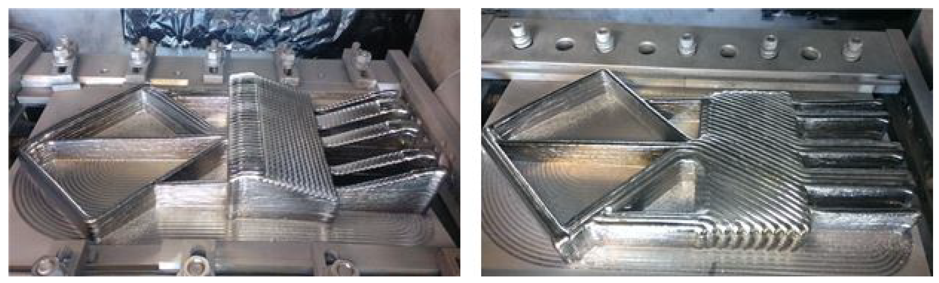
Figure 1.
Electron beam additive manufacturing notional part geometry measuring 40 cm in width, 72 cm in length, and 18 cm in height; top (left) and bottom (right).
Figure 2.
Distortion of NP1 fabricated using EBAM technology on a 1.27 cm plate; part geometry measures 40 cm in width and 18 cm in height. Thermal cycling and the weight of the printed material have permanently deflected the base plate as shown.
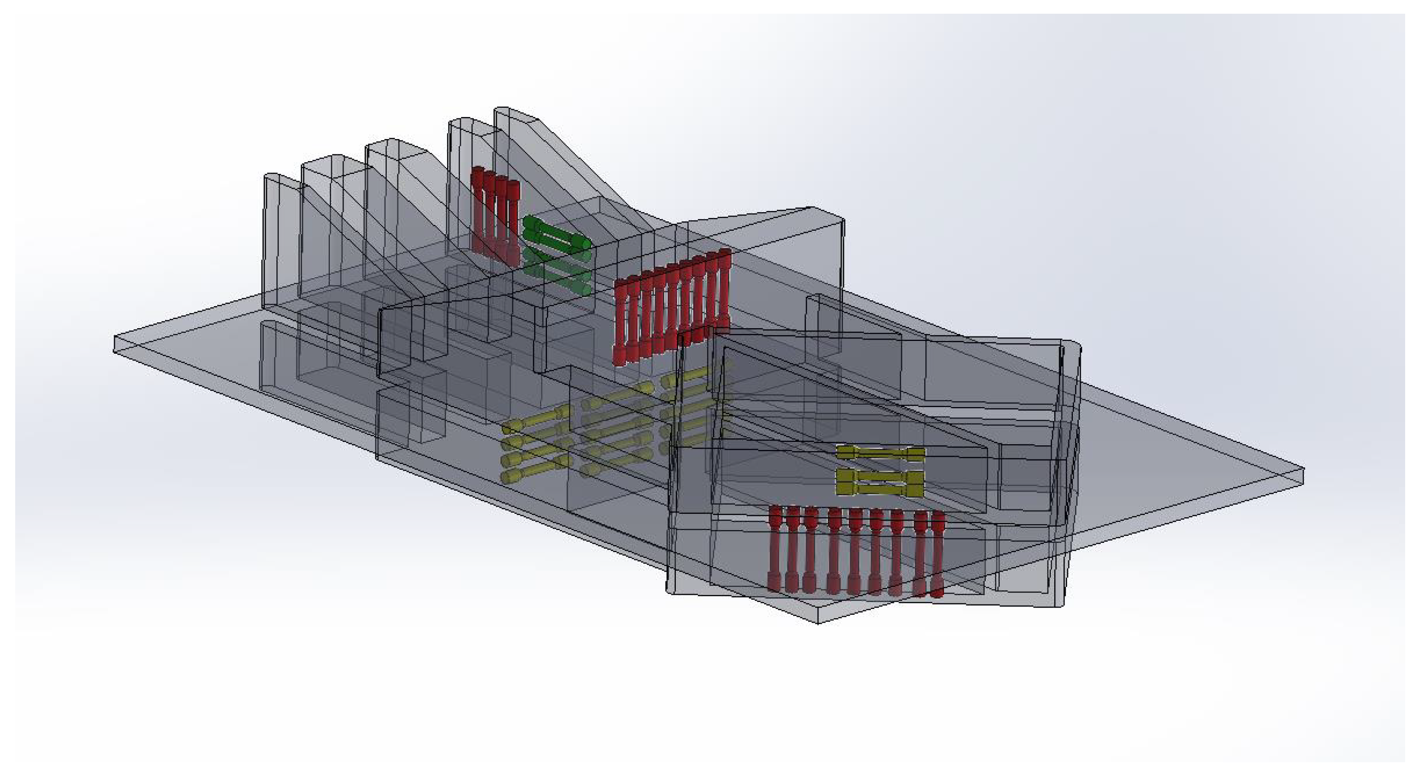
Figure 3.
3D representation of the as-printed part with the tensile test specimen locations isolated. Red are vertically oriented specimens in the z-direction, yellow are horizontally oriented across the body in an x-y plane, and green are purely horizontal specimens either in x or y-directions. The part geometry measures 40 cm in width, 72 cm in length, and 18 cm in height.
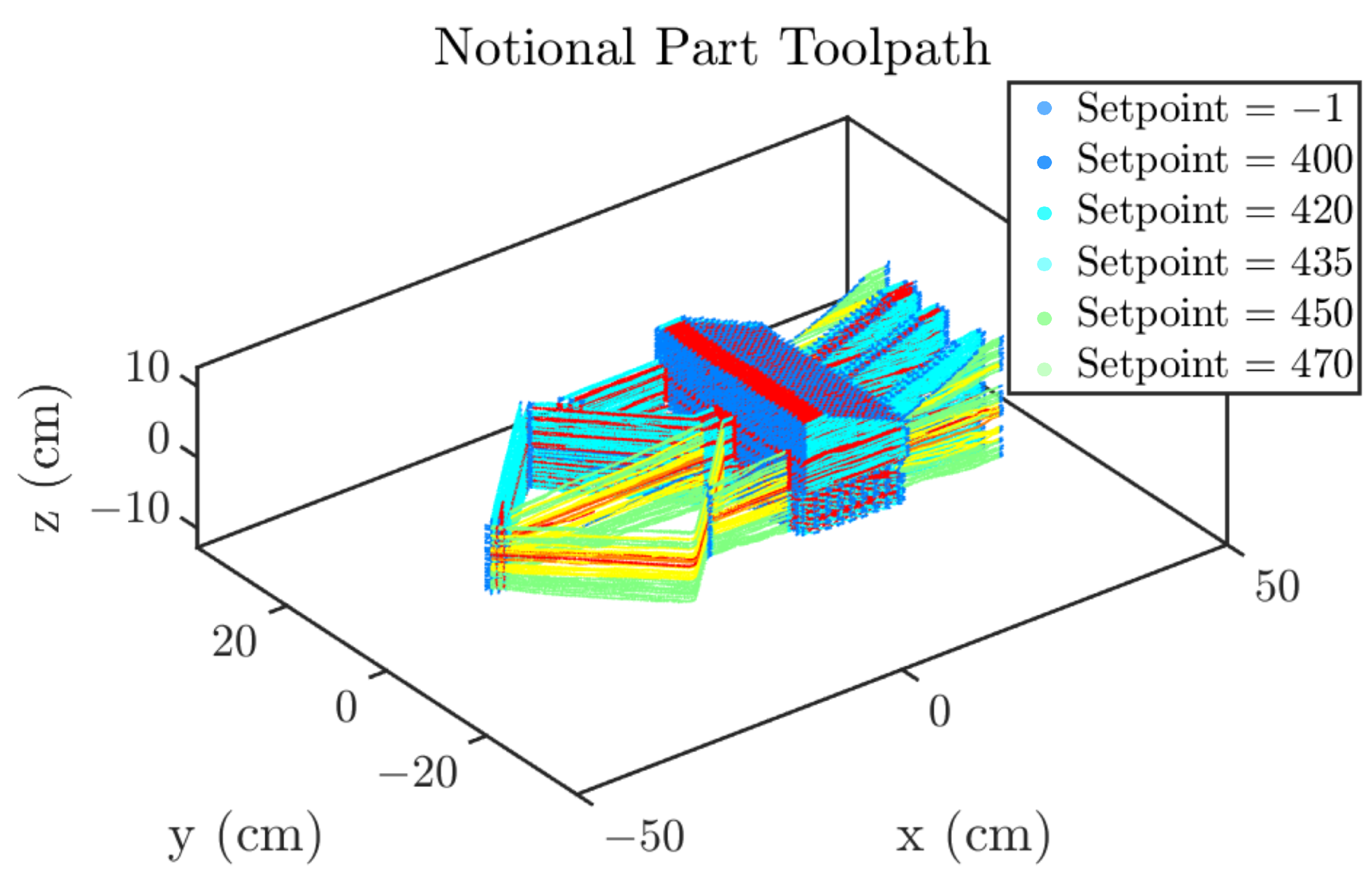
Figure 4.
Setpoint locations for NP3 to show the continuity of the printed part.
Figure 5.
Predicted versus measured and (MPa) for the NP1 horizontal and vertical specimens.
Figure 6.
Predicted versus measured and (MPa) for the NP2 horizontal and vertical specimens.
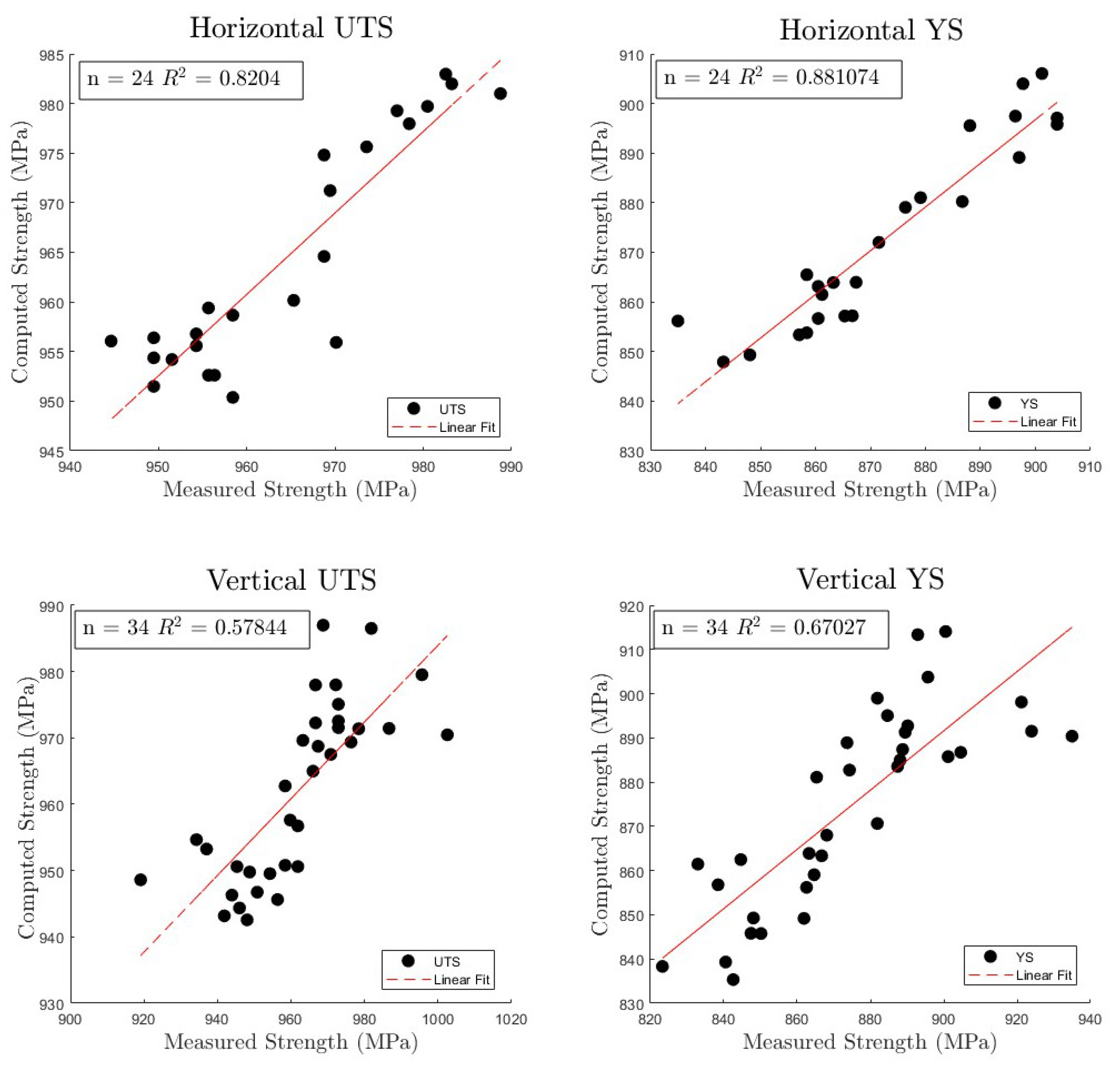
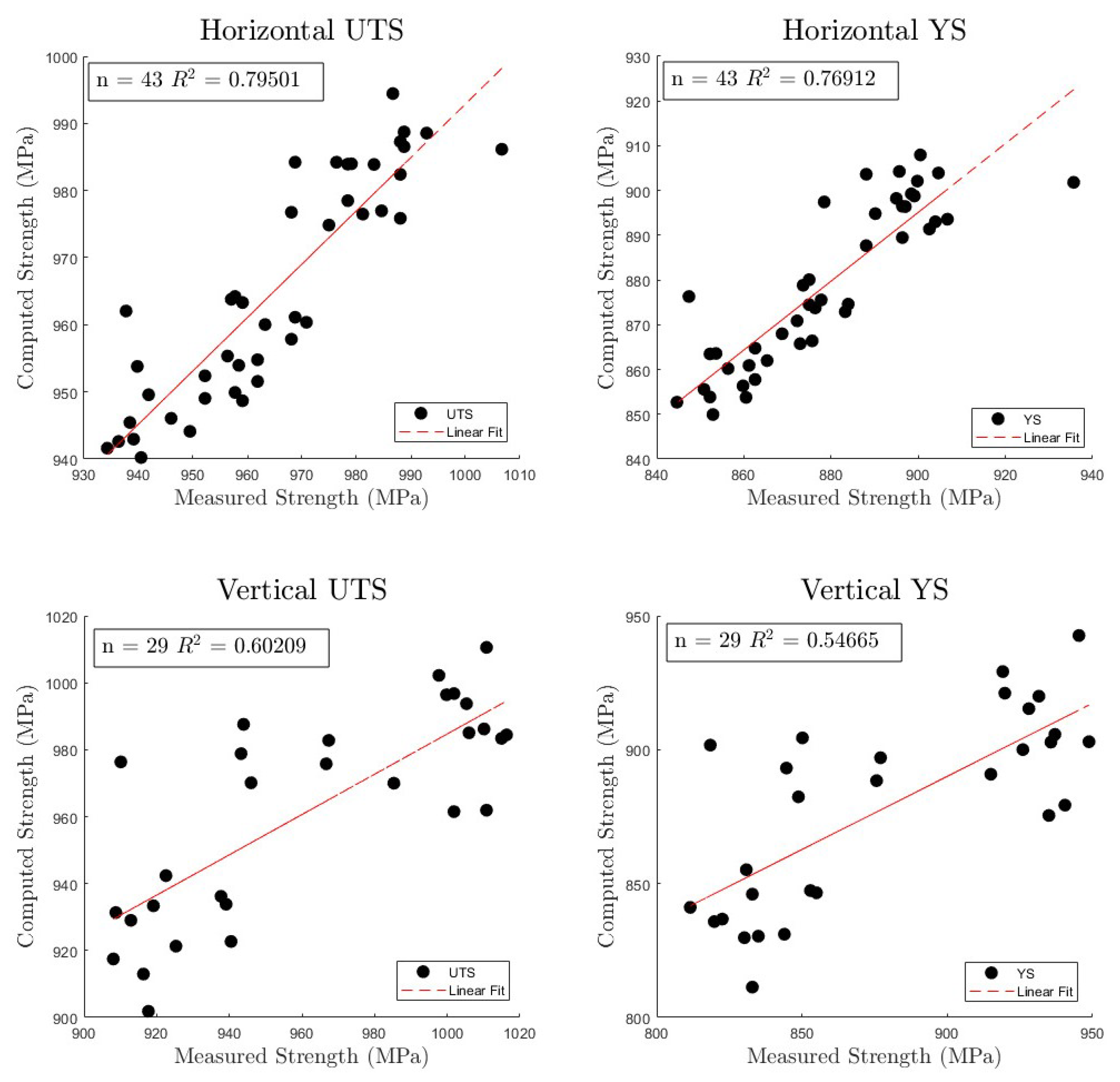
Figure 7.
Predicted versus measured and (MPa) for the NP3 horizontal and vertical specimens.
Table 1.
Measured values and standard deviations of the print conditions.
| Measured Parameter | Average | Standard Deviation |
|---|
| 39.95 kV | 0.19 kV |
| 3.43 A | 0.002 A |
| 459.9 pixels | 54.52 pixels |
| 42.79 μTorr | 16.15 μTorr |
| 218.8 mA | 15.65 mA |
Table 2.
Total number of data points available for NP1 through NP3. The setpoints 400 through 470 are continuous on the top and bottom of the print, while the points marked with a −1 are when the processing parameters were not used in the predictive model.
| Setpoint | NP1 | NP2 | NP3 |
|---|
| 400 | 3446 | 29,044 | 6414 |
| 410 | − | 65,750 | − |
| 415 | − | 19,972 | − |
| 420 | − | 9798 | 17,514 |
| 435 | 153,865 | 14,178 | 10,230 |
| 450 | − | − | 2323 |
| 470 | 284,333 | 258,148 | 171,818 |
| −1 | 182,959 | 134,437 | 102,053 |
| Total | 624,603 | 531,327 | 368,079 |
Table 3.
values for predicted and for the horizontal and vertical components utilizing a range of values for the volume in the z, or vertical, direction in order to optimize the accuracy of the predicted results for all components of the stresses.
| Thickness | Horizontal | Horizontal | Vertical | Vertical | Sum |
|---|
| 0.254 | 0.48297 | 0.48039 | 0.66939 | 0.59814 | 2.231 |
| 0.508 | 0.46945 | 0.46914 | 0.67837 | 0.60905 | 2.226 |
| 0.762 | 0.44363 | 0.43299 | 0.66684 | 0.59553 | 2.139 |
| 1.016 | 0.45156 | 0.44167 | 0.65951 | 0.58557 | 2.138 |
| 1.27 | 0.45388 | 0.44123 | 0.65836 | 0.58341 | 2.137 |
| 1.524 | 0.44743 | 0.43892 | 0.65806 | 0.58263 | 2.127 |
| 1.778 | 0.43625 | 0.42538 | 0.65813 | 0.58228 | 2.102 |
| 2.032 | 0.42746 | 0.41469 | 0.65846 | 0.58222 | 2.083 |
| 2.286 | 0.42276 | 0.41107 | 0.65841 | 0.58222 | 2.074 |
| 2.54 | 0.41860 | 0.40741 | 0.65844 | 0.58222 | 2.067 |
| 2.794 | 0.41481 | 0.40429 | 0.65857 | 0.58222 | 2.059 |
| 3.302 | 0.40580 | 0.39344 | 0.65913 | 0.58234 | 2.041 |
| 3.81 | 0.39244 | 0.37627 | 0.66003 | 0.58269 | 2.011 |
| 4.572 | 0.37177 | 0.34735 | 0.65927 | 0.58232 | 1.961 |
| 5.08 | 0.35905 | 0.32865 | 0.65859 | 0.58222 | 1.926 |
Table 4.
The number of points in the data set, n, for the linear regression model and their associated correlation coefficient, , for NP1.
| Direction | Stress | n | |
|---|
| horizontal | | 28 | 0.48297 |
| horizontal | | 28 | 0.48039 |
| vertical | | 21 | 0.6694 |
| vertical | | 21 | 0.59814 |
Table 5.
Calculated coefficients for the linear regression models of horizontal and vertical components of and in NP1.
| Component | | | | | | | | | |
|---|
| 144.99 | 195.9 | −3.08 | 8.24 | 3.04 | 0.009 | 298.83 | 48.67 | 3.06 |
| 961.01 | 169.1 | −10.79 | 13.58 | 3.94 | −0.008 | 283.29 | 70.03 | 4.89 |
| 11,855 | 377.2 | 0.27 | −1.14 | −20.33 | −0.534 | 420.48 | −28.31 | −7543.24 |
| 19,365 | 586.8 | −0.37 | 2.39 | −28.56 | −0.728 | 625.16 | −34.92 | −12,576.41 |
Table 6.
values for predicted and for the horizontal and vertical components utilizing a range of values for the volume in the z, or vertical, direction in order to optimize the accuracy of the predicted results for all components of the stresses.
| Thickness | Horizontal | Horizontal | Vertical | Vertical | Sum |
|---|
| 0.254 | 0.8204 | 0.88106 | 0.57844 | 0.670265 | 2.9502 |
| 0.508 | 0.8251 | 0.8813 | 0.5776 | 0.657984 | 2.94203 |
| 0.762 | 0.8221 | 0.8809 | 0.57172 | 0.65632 | 2.93115 |
| 1.016 | 0.82104 | 0.87877 | 0.5717 | 0.65632 | 2.9288 |
| 1.27 | 0.81717 | 0.87742 | 0.56872 | 0.65052 | 2.9138 |
| 1.524 | 0.8177 | 0.875617 | 0.57077 | 0.65371 | 2.9178 |
| 1.778 | 0.82217 | 0.875827 | 0.56821 | 0.64999 | 2.9162 |
| 2.032 | 0.82309 | 0.87478 | 0.5679 | 0.64961 | 2.9154 |
| 2.286 | 0.82777 | 0.874 | 0.56776 | 0.64963 | 2.9191 |
| 2.54 | 0.83414 | 0.87328 | 0.56583 | 0.64648 | 2.9197 |
| 2.794 | 0.84046 | 0.87343 | 0.56432 | 0.64392 | 2.92215 |
| 3.302 | 0.85283 | 0.873002 | 0.56238 | 0.64025 | 2.9284 |
| 3.81 | 0.86276 | 0.87265 | 0.56184 | 0.63991 | 2.9371 |
| 4.572 | 0.869285 | 0.87195 | 0.56125 | 0.639405 | 2.9419 |
| 5.08 | 0.86991 | 0.871075 | 0.56121 | 0.639317 | 2.9415 |
Table 7.
Calculated coefficients for the linear regression models of horizontal and vertical components of and for NP2.
| Component | | | | | | | | | |
|---|
| 0 | 42.5 | 0.8 | 0.04 | 0.6 | 0.05 | 80.9 | 10.3 | 2.26 |
| 0 | 212.4 | −4.06 | 16.1 | 1.9 | 0.2 | 338.3 | 18.01 | 1.51 |
| 0 | 254.9 | −34.7 | 28.3 | 7.5 | −0.07 | 639.4 | −4.8 | 2302.2 |
| 0 | 259.7 | −89.8 | 10.5 | 7.9 | −0.27 | 772.8 | −2.3 | 7036.4 |
Table 8.
The number of points in the NP2 data set, n, for the linear regression model and their associated correlation coefficient, .
| Direction | Stress | n | |
|---|
| horizontal | | 24 | 0.8204 |
| horizontal | | 24 | 0.88107 |
| vertical | | 34 | 0.57844 |
| vertical | | 34 | 0.67027 |
Table 9.
values for predicted and for the horizontal and vertical components utilizing a range of values for the volume in the z, or vertical, direction in order to optimize the accuracy of the predicted results for all components of the stresses.
| Thickness | Horizontal | Horizontal | Vertical | Vertical | Sum |
|---|
| 0.254 | 0.795 | 0.769122 | 0.60208 | 0.54664 | 2.71286 |
| 0.508 | 0.79141 | 0.762864 | 0.6024 | 0.54781 | 2.7045 |
| 0.762 | 0.78721 | 0.756946 | 0.59989 | 0.54614 | 2.69019 |
| 1.016 | 0.78471 | 0.752357 | 0.59515 | 0.54179 | 2.67401 |
| 1.27 | 0.78308 | 0.74943 | 0.58938 | 0.53638 | 2.6582 |
| 1.524 | 0.78201 | 0.74723 | 0.58491 | 0.5325 | 2.64665 |
| 1.778 | 0.781015 | 0.745832 | 0.58086 | 0.52923 | 2.6369 |
| 2.032 | 0.78026 | 0.744923 | 0.57887 | 0.52775 | 2.6318 |
| 2.286 | 0.77975 | 0.744795 | 0.57693 | 0.52642 | 2.6279 |
| 2.54 | 0.77979 | 0.745767 | 0.57483 | 0.525145 | 2.6255 |
| 2.794 | 0.78067 | 0.748375 | 0.57369 | 0.52462 | 2.6274 |
| 3.302 | 0.78539 | 0.757894 | 0.57218 | 0.52444 | 2.6399 |
| 3.81 | 0.792701 | 0.7708 | 0.57164 | 0.52517 | 2.6603 |
| 4.572 | 0.80319 | 0.786155 | 0.57178 | 0.52663 | 2.6878 |
| 5.08 | 0.80905 | 0.793216 | 0.572009 | 0.527404 | 2.7017 |
Table 10.
Calculated coefficients for the linear regression models of horizontal and vertical components of and .
| Component | | | | | | | | | |
|---|
| 97.3 | 96.33 | −0.69 | 3.2 | −1.7 | 0.061 | −40.7 | −16.2 | −2.17 |
| 76.8 | 119.2 | −0.96 | 4.3 | −1.9 | 0.064 | −23 | −21.2 | −3.01 |
| −7960 | −166.2 | −2.1 | 5.2 | −2.8 | 0.42 | −233.9 | −2.31 | 5288.6 |
| −8217.7 | −160.5 | −2.7 | 6.7 | −1.7 | 0.55 | −237.4 | 7.16 | 5455.6 |
Table 11.
Comparison of the correlation coefficient, , between successive prints, NP1, NP2, and NP3.
| Direction | Stress | -NP1 | -NP2 | -NP3 |
|---|
| horizontal | | 0.48297 | 0.8204 | 0.79501 |
| horizontal | | 0.48039 | 0.88107 | 0.76912 |
| vertical | | 0.6694 | 0.57844 | 0.60209 |
| vertical | | 0.59814 | 0.67027 | 0.54665 |
| Publisher’s Note: MDPI stays neutral with regard to jurisdictional claims in published maps and institutional affiliations. |
© 2022 by the authors. Licensee MDPI, Basel, Switzerland. This article is an open access article distributed under the terms and conditions of the Creative Commons Attribution (CC BY) license (https://creativecommons.org/licenses/by/4.0/).


