Studies on Parameters Affecting Temperature of Liquid Steel and Prediction Using Modified AdaBoost.RT Algorithm Ensemble Extreme Learning Machine

Abstract

The present work aimed to develop a predictive model for the end temperature of liquid steel in advance to support the smooth functioning of a vacuum tank degasser (VTD). An ensemble model that combines extreme learning machine (ELM) with a self-adaptive AdaBoost.RT algorithm was established for the regression problem. Based on analyzing the energy equilibrium of the VTD system, the factors were determined for predicting the end temperature of liquid steel. To establish a hybrid ensemble prediction model, an ELM algorithm was selected as the ensemble predictor due to its strong performance and robustness, and a modification of the AdaBoost.RT algorithm is proposed to overcome the drawback of the original AdaBoost.RT by embedding statistical theory to dynamically self-adjust the threshold value. For efficient VTD operations, an ensemble model that combines ELM with the self-adaptive AdaBoost.RT algorithm was established to model the end temperature of liquid steel. The proposed approach was analyzed and validated on actual production data derived from a steelmaking workshop in Baosteel. The experimental results reveal that the proposed model can improve the generalization performance, and the accuracy of the model is feasible for the secondary steel refining process. In addition, a polynomial equation is obtained from the ensemble predictive model for calculating the value of the end temperature. The predicted results are in good agreement with the actual data with <1.7% error.

1. Introduction

In modern life, the new materials market has become highly competitive. As a result, clean steel has been increasingly important in the steel industry and plays a vital role in defending steel products against newer competitive materials [1,2,3,4,5]. To produce steel with satisfactory cleanliness and low contents of impurities, such as sulfur, phosphorus, non-metallic inclusions, hydrogen and nitrogen, it is necessary to precisely control the composition and temperature of liquid steel [6,7]. Steelmakers are urged to improve operating conditions throughout the steelmaking process, such as by applying deoxidant and alloy additions, secondary metallurgy treatments and casting strategies, to obtain high-purity steel [8]. In practice, vacuum tank degassing (VTD) is widely used as a secondary steelmaking process to produce products with low contents of carbon, hydrogen and nitrogen [9,10,11].

The main purpose of the VTD refining process is to obtain qualified liquid steel with the desired composition and temperature. A method for improving the temperature control level of liquid steel in VTD is to accurately predict the temperature. The degassing process in VTD, as the most critical step in the production of clean steel, has been investigated in a number of studies using various approaches with the goal of better understanding the effect of process parameters and thus further improving the energy efficiency. Several mathematical models of VTD refining have been developed [12,13,14]. These models were formulated as a series of differential equations to describe the chemical and physical changes occurring in the zone of the ladle. VTD is a typical nonlinear system, and some of the mechanisms are still not very well understood. It is indeed very difficult or even impossible to establish a standard mathematical model to encompass all of the dynamics of a VTD process. These mathematical models are local models of dehydrogenation [13] or denitrogenation [14], which describe only some of the properties and are time-consuming in their calculations, so it is almost impossible to predict the temperature of liquid steel using these kinds of models.

An artificial neural network (ANN) is an information processing mechanism [15] used to define a mathematical relationship between process inputs and outputs that “learn” directly from historical data. ANNs have been widely applied in the steelmaking process. Gajic et al. [16], for instance, have constructed an energy consumption model of an electric arc furnace (EAF) based on feedforward ANNs. Temperature prediction models [17,18] for EAF were established by using neural networks. Rajesh et al. [19] employed feedforward neural networks to predict the intermediate stopping temperature and end-blow oxygen in the LD converter steelmaking process. Wang et al. [20] have developed a liquid steel temperature prediction model in a ladle furnace by using general regression neural networks as the predictor in their ensemble method. Our previous work [21] relied on the end-temperature classification of VTD by using classification and regression trees (CARTs) and extracted operation rules for decision making in the process. The main feature that makes neural nets a suitable approach for predicting the end temperature of liquid steel in VTD is that they are nonlinear regression algorithms and can model high-dimensional systems. These black-box models offer alternatives to traditional concepts of knowledge representation to solve the prediction problem for an industrial production process system.

Nowadays, ensemble technologies such as Bagging [22] and Boosting [23] are broadly used to obtain far better performance in classification and regression problems than a single classifier and regressor. The AdaBoost (short for Adaptive Boosting) algorithm is one of the most prevalent boosting methods and was originally developed for binary classification issues [23]. As extensions of AdaBoost, AdaBoost.M1 and AdaBoost.M2 were proposed to deal with multi-classification problems. The main idea of the AdaBoost algorithm is voting based on the weights of weak classifiers in terms of their corresponding training errors to generate an aggregated classifier. This combination of weak classifiers is stronger than any single one.

For regression issues, AdaBoost.R is extended from AdaBoost.M2 by transforming the regression sample into a classification label space. In addition, Drucker [24] improved AdaBoost.R to AdaBoost.R2 by considering the loss function to calculate the error rate of a weak regressor. Additionally, Solomatine and Shrestha [25] proposed AdaBoost.RT (R and T stand for regression and threshold) by introducing a constant threshold ϕ to demarcate the samples as correct and incorrect predictions. The predictions of samples with an absolute relative error less than the threshold ϕ are marked as correct predictions; otherwise, they are regarded as incorrect. According to Shrestha and Solomatine’s experiments [26], the committee machine is stable when the value of ϕ is between 0 and 0.4. To accurately select the threshold value, Tian and Mao [27] presented a modified AdaBoost.RT algorithm by using a self-adaptive modification mechanism subjected to the change trend of the prediction error at each iteration. This approach has performed well in predicting the temperature of liquid steel in a ladle furnace, but the initial value of ϕ₀ also needs to be manually fixed. Moreover, Zhang and Yang [28] proposed a robust AdaBoost.RT by considering the standard deviation of approximation errors to determine the threshold. The absolute error is used to demarcate the samples as either well or poorly predicted in this approach. The method has performed well on regression problems from the UCI Machine Learning Repository [29]. In our study, a method for the dynamic self-adjustable modification of the value of ϕ was used instead of the invariable ϕ to improve the original AdaBoost.RT algorithm.

In the present work, to estimate the relative error of samples, a variation coefficient (σ/μ) of the predictions at each iteration is proposed instead of the constant threshold ϕ in the original AdaBoost.RT algorithm. An adjustable relative factor λ is introduced to make the threshold value stable. Therefore, the credible threshold for the absolute relative error is λσ/μ in our study. This threshold is applied to demarcate samples as either correct or incorrect predictions, and the value is self-adjusted to the prediction performance of the training samples. The structure of the work is presented as follows. Firstly, the impacts of the ladle conditions and process parameters on the end temperature of liquid steel are studied by analyzing the process flow and energy equilibrium of the VTD system. Subsequently, an extreme learning machine (ELM) network is presented for the regression problem, and a modified AdaBoost.RT algorithm that embeds statistical theory is introduced to dynamically self-adjust the threshold value. Then, an ensemble model that combines ELM with the self-adaptive AdaBoost.RT algorithm is established to model the end temperature of liquid steel. In the Section 3, the proposed hybrid ensemble prediction model is validated on actual production data derived from a steelmaking workshop in Baosteel. The application of the ensemble model, a sensitivity analysis of the process parameters, is presented in the Section 4. Finally, conclusions are drawn in the Section 5.

2. VTD Refining Process and Modeling Methods

2.1. VTD Refining Process

2.1.1. Energy Conservation of VTD

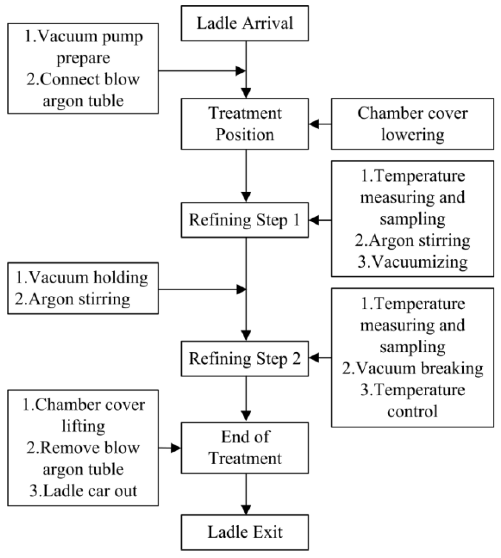
To develop the intelligent temperature prediction model, the whole VTD refining process is considered an energy conservation system. The practical refining process of VTD is illustrated in Figure 1. To accurately control the composition and temperature, the temperature is measured at different times for different types of steel. Therefore, we chose the time of the last temperature measurement before the ladle is placed into the vacuum chamber as the start time of the energy conservation system, and this temperature is the initial temperature. The ending time is the time of the last temperature measurement.

As depicted in the VTD refining process in Figure 1, there is no other energy added to the ladle during the VTD refining process. Therefore, the VTD refining process is defined as an energy loss process. The temperature of liquid steel is decreased in VTD due to the energy loss during the refining process. The energy conservation of VTD is depicted in Figure 2. The output energy of the VTD system is the heat loss from the top surface (Q_surf), the heat loss due to argon stirring (Q_argon), the heat loss of the gas used during vacuumizing and vacuum breaking (Q_gas) and the heat loss from the ladle refractory lining, which is composed of two parts: heat content absorbed by the ladle lining (Q_ladle) and convection loss to the atmosphere from the ladle shell (Q_shell). The temperature of liquid steel is decreased due to the total energy loss of the VTD system (Q), as calculated in the following formula.

Q = Q_surf + Q_argon + Q_gas + Q_ladle + Q_shell

(1)

2.1.2. Factors of Liquid Steel Temperature

Through the analysis of the practical refining process and the energy conservation of the VTD system, the influencing factors of the liquid steel temperature in VTD are further clarified. There are eight factors affecting the temperature of liquid steel in VTD: the steel grade, ladle conditions, the weight of liquid steel, the initial temperature of liquid steel in VTD, refining time, vacuumizing time, vacuum holding time and argon gas consumption.

Of the above eight factors, the steel grade and ladle conditions are the two discrete parameters that have a significant influence on the temperature of liquid steel. The ladle heat conditions are listed in

Table 1. The division of ladle conditions.

Ladle Conditions	Ladle Class	Description	Code Levels
		Ordinary ladle	−1
Ladle material		Cord ladle	0
		Ladle for VOD (vacuum oxygen decarburization)	1
	Prior period	The ladle is used in 1–6 furnaces.	−1
Refractory life	Mid-term	The ladle is used in 7–12 furnaces.	0
	Last stage	The ladle is used in more than 13 furnaces.	1
		(0 < T1 ≤ 3 h, T2= 0 h)
	Hot	(3 < T1 ≤ 4 h, T2 = 1 h), (4 < T1 ≤ 5 h, T2 = 2 h), (5 < T1 ≤ 6 h, T2 = 3 h)	−1
		(3 < T1 ≤ 4 h, T2 = 0 h), (4 < T1 ≤ 5 h, T2 = 1 h), (5 < T1 ≤ 6 h, T2 = 2 h)
Heat status	Normal	(4 < T1 ≤ 5 h, T2 = 0 h), (5 < T1 ≤ 6 h, T2 ≤ 1 h)	0
		(6 < T1 ≤ 10 h, T2 < T1 − 4)
	Cold	(T1 ≥ 10 h)	1
		New ladle

T₁ denotes the time interval from the end of casting to the next tapping of the converter. T₂ denotes the time of ladle preheating.

.

As tabulated in Table 1, there are three main types of ladle conditions, i.e., ladle material, refractory life and heat status. In the practical refining process, the ladle used in 1–6 furnaces denotes the prior period of the ladle, that used in 7–12 furnaces denotes the mid-term, and the ladle used in more than 13 furnaces denotes the last stage of the ladle. To consider these discrete variables in our prediction model, each factor was varied at three levels: the lowest level (−1), the middle level (0) and the highest level (1). The independent discrete variables’ corresponding coded levels are shown in Table 1.

2.2. Ensemble ELM with Self-Adaptive AdaBoost.RT Algorithm

2.2.1. Extreme Learning Machine

Extreme learning machine (ELM) [30] is an efficient learning algorithm for single-hidden-layer feedforward neural networks (SLFNs). Based on the least-square method, the ELM algorithm can run without iterative tuning and reach a globally optimal solution with a much faster learning speed. The input weights and the hidden layer biases are selected randomly, and the output weights between the hidden layer and output layer are determined analytically during the learning process [31]. The computing procedure of ELM denotes Algorithm 1 and is described as follows.

Algorithm 1: Learning Routine of ELM for Regression

1. Input:

Given a training data set comprising N observations {xn}, where n = 1,..., N, together with corresponding target values {yn}, the goal is to predict the value of t for a new value of x.

The activation function of hidden layer G(wi, bi, xj).

The regularization coefficient C.

The hidden node number L.

2. Initialize:

The hidden layer output with L nodes can be presented by a row vector h(x) = [h1(x), …, hL(x)].

The mathematical model of the SLFNs can be described as Hβ = Y, where H is the hidden layer output matrix, β is the output weight and Y is the target vector.

Randomly generate the input weight vector wi and bias bi based on some continuous distribution to form the hidden layer output matrix of network $\mathit{H}=\left[\begin{array}{c}\mathit{h}\left({\mathit{x}}_1\right)\\ ⋮\\ \mathit{h}\left({\mathit{x}}_N\right)\end{array}\right]={\left[\begin{array}{ccc}G\left({\mathit{w}}_1,b_1,{\mathit{x}}_1\right)& \cdots & G\left({\mathit{w}}_L,b_L,{\mathit{x}}_1\right)\\ ⋮& ⋮& ⋮\\ G\left({\mathit{w}}_1,b_1,{\mathit{x}}_N\right)& \cdots & G\left({\mathit{w}}_L,b_L,{\mathit{x}}_N\right)\end{array}\right]}_{N\times L}$

3. Calculate:

As defined in ELM, the aim of ELM is to calculate the weight vector β in minimizing the training error as well as the norm of outputs weights. The mathematical problem can be represented as: $\begin{array}{cc}Minimize& L_{P_{ELM}}=\frac{1}{2}{\left|\right|\mathit{\beta }\left|\right|}^2+\frac{C}{2}\sum _{i=1}^N{\xi }_i^2\\ Subject to& \mathit{h}\left({\mathit{x}}_i\right)\beta =y_i-{\xi }_i,i=1, 2,\dots , N.\end{array}$

The least-square solution with minimal norm is analytically determined using Moore–Penrose “generalized” inverse: $\mathit{\beta }={\mathit{H}}^T{\left(\frac{I}{C}+\mathit{H}{\mathit{H}}^T\right)}^{-1}Y, when N<L$; $\mathit{\beta }={\left(\frac{\mathit{I}}{C}+{\mathit{H}}^T\mathit{H}\right)}^{-1}{\mathit{H}}^{T}Y, when N>L$.

4. Output:

f(x) = h(x)β

2.2.2. Self-Adaptive AdaBoost.RT Algorithm

As detailed in Section 1, a comparison of the threshold determination methods in different AdaBoost.RT algorithms is given in

Table 2. Comparison of the threshold determination methods in different AdaBoost.RT algorithms.

Algorithms	Determination Method of Threshold	Description
AdaBoost.RT [26]	$\left|\frac{f_t\left(x_i\right)-y_i}{y_i}\right|\le \varphi$	Constant threshold, must specify the value ϕ ∈ (0, 0.4).
Modified AdaBoost.RT [27]	$\{\begin{array}{cc}{\varphi }_{t+1}=\left(1-\lambda \right){\varphi }_t,& e_t<e_{t-1}\\ {\varphi }_{t+1}=\left(1+\lambda \right){\varphi }_t,& e_t>e_{t-1}\end{array}$	The value of threshold changes with error rate at each iteration but should specify the initial value ϕ0 = 0.2.
Robust AdaBoost.RT [28]	$\left|f_t\left(x_i\right)-y_i\right|\le \frac{1}{2}{\sigma }_t$	Absolute error is the evaluation criterion, and threshold value changes according to the standard deviation.
Proposed method	$\left|\frac{f_t\left(x_i\right)-y_i}{y_i}\right|\le \lambda \frac{\sigma }{\mu }$	Automatic selection of threshold value according to the coefficient of variation.

. According to our previous work and prior experimental research results [32], the coefficient of variation (σ/μ) can be used as the evaluation criterion of absolute relative error. In this paper, a relative factor, λ, is introduced to maintain the stable adjustment of the threshold value, which results in the self-adaptive threshold λσ/μ.

To effectively determine the threshold value ϕ in the original AdaBoost.RT algorithm, a novel modification of AdaBoost.RT is proposed in the present work. We embedded the statistical theory related to the regression capability of the weak learner into the AdaBoost.RT algorithm. A method for the dynamic self-adjustable modification of the value of ϕ is used instead of the invariable ϕ. The computing procedure of the proposed self-adaptive AdaBoost.RT algorithm is described as follows.

Algorithm 2: Learning Routine of the Modified AdaBoost.RT

1. Input:

Training data sets with m samples (x1, y1), …, (xm, ym), where output yi ∈ R.

Weak learning algorithm (ELM in this work).

The maximum number of iterations (machines) T.

2. Initialize:

Machine number or iteration t = 1.

Distribution Dt(i) = 1/m for all i.

Error rate ɛt = 0.

3. Iterate while t ≤ T:

Train ELM to build the regression model: ft(x) → y.

Calculate absolute relative error (ARE) for each training sample as AREt(i) = |(ft(xi) − yi)/yi|.

Calculate the weak learner’s error rate as ${\epsilon }_t=\sum _{i\in H_t}{D}_t\left(i\right)$.

The set of erroneous samples Ht in our proposed method is $H_t\left\{i|\left|\left(f_t\left({\mathit{x}}_i\right)-y_i\right)/y_i\right|>\lambda {\sigma }_t/{\mu }_t\right\}$.

μt is the sample mean value of the predictive values on the training set ft(xi); σt is the sample standard deviation of (ft(xi) − yi) in the tth network. The relative factor λ is defined as λ ∈ (0, 1) and can be determined by users for different regression problems.

Calculate the fraction error βt = ɛt/(1 − ɛt) and update the training sample weight Dt+1(i) as $D_{t+1}\left(i\right)=\frac{D_t\left(i\right)}{Z_t}\{\begin{array}{cc}{\beta }_t& if \left|\left(f_t\left({\mathit{x}}_i\right)-y_i\right)/y_i\right|\le \lambda {\sigma }_t/{\mu }_t\\ 1& otherwise\end{array}$

where Zt is a normalization factor chosen such that Dt+1 will be a distribution.

Set t = t + 1.

4. Output the final hypothesis function:

$f_{fin}\left(\mathit{x}\right)={\displaystyle \sum _t}log\left(1/{\beta }_t\right)f_t\left(\mathit{x}\right)/{\displaystyle \sum _t}log\left(1/{\beta }_t\right)$

The critical threshold used in the boosting process of Algorithm 2 becomes self-adaptive to the individual weak learners’ performance on the input data samples. In probability and statistical theory, most of the relative errors of predictions of the tth weak learner will be located within the range [−σ_t/μ_t, +σ_t/μ_t]. Thus, the variation coefficient (σ/μ) of the predictions at each iteration can be used as a criterion to estimate the relative error of the samples. To make the threshold value stable, an adjustable relative factor, λ, which ranges from 0 to 1, is introduced to the variation coefficient. Therefore, the credible threshold for the absolute relative error becomes λσ/μ. This self-adaptive threshold is applied to demarcate samples as either correct or incorrect predictions. If the absolute relative error for any particular sample is greater than the threshold, this predictive value is rejected, and the learning weight will be increased in the next iteration. This makes it easy to give more attention to harder examples.

The key difference between self-adaptive AdaBoost.RT and robust AdaBoost.RT [28] is computing the prediction error rate using the absolute relative error rather than the absolute error. This makes it possible to place enough emphasis on the samples when the values are very low. Moreover, an adjustable relative factor, λ, is utilized to modify the threshold according to the predicted results at each iteration. Lastly, by introducing the credible threshold, the algorithm will be stable and work efficiently on the production date of the industrial process.

2.2.3. Ensemble ELM Based on Self-Adaptive AdaBoost.RT

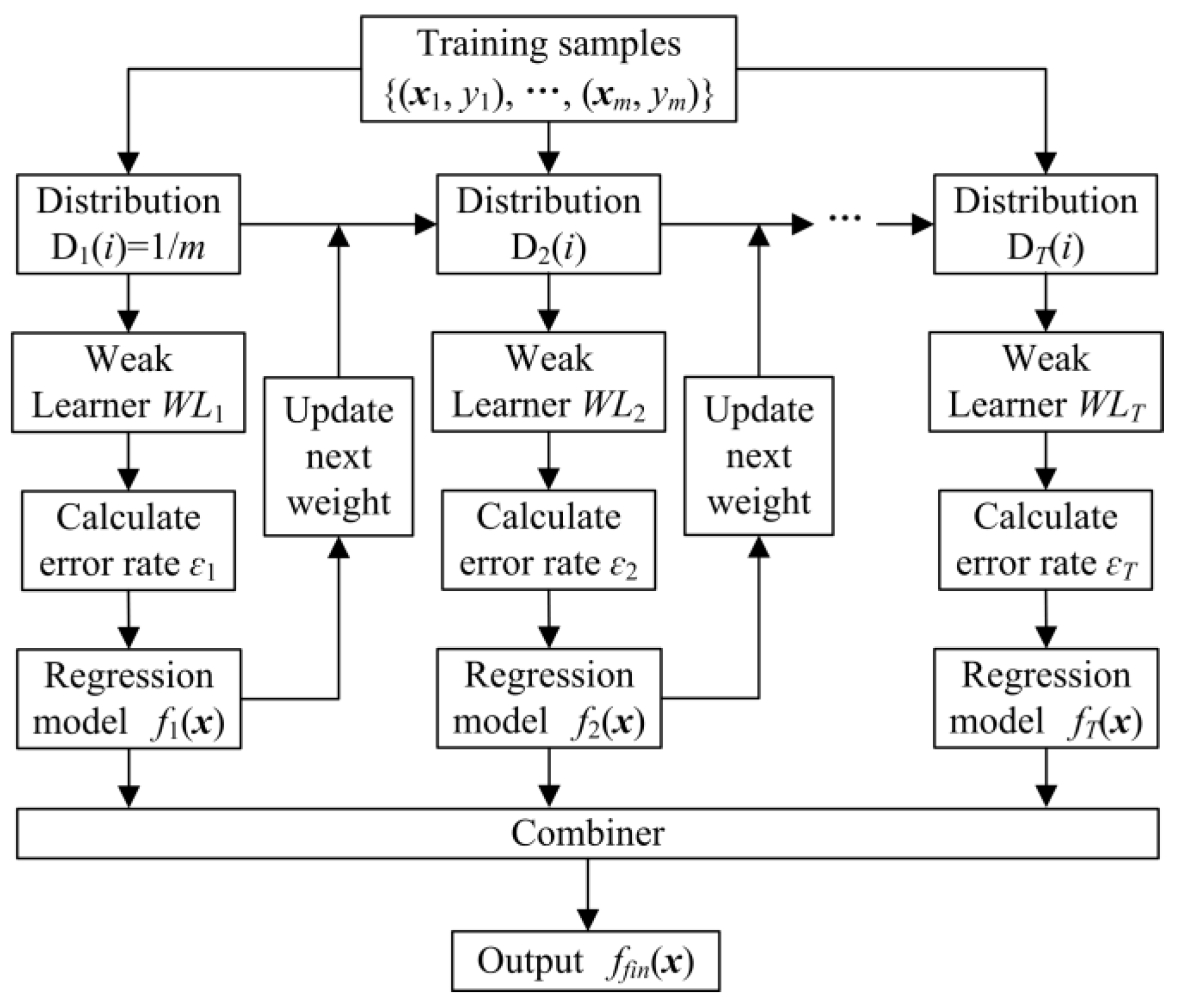
In this work, a self-adaptive AdaBoost.RT ensemble ELM (SAE-ELM) was developed to obtain the end temperature of liquid steel in VTD from a large set of plant operating parameters. Here, ELM is used as the “weak learner”, and self-adaptive AdaBoost.RT is the ensemble method. The proposed ensemble model is illustrated in Figure 3.

Initialization: A training data set with m samples is applied to train the prediction model. For the first iteration, the weights of the samples are uniform so that each sample is chosen with an equal probability in the first round.

Update of the distribution: The prediction error of the weak learner at the tth iteration is evaluated by the relative error rate. The self-adaptive threshold λσ_t/μ_t is applied to demarcate the samples as either correct or incorrect predictions. For samples that are correctly predicted by the current weak learner, the corresponding weights are multiplied by the error rate function β_t. Otherwise, the weights do not change. According to the fraction error β_t, the samples with incorrect predictions are granted a larger weight in the next iteration. This process is iterated until the last weak learner.

Integration of the final prediction results: To obtain a better predictive performance model than the weak learner, the hybrid SAE-ELM model combines each iteration’s weak learner with different weights as the final hypothesis.

3. Experiments and Results

3.1. Variables and Data

A total of 2963 observations of six kinds of steel during normal operations in VTD were collected for modeling purposes. Each observation contains ladle conditions and eight continuous process parameters. After removing the blank data, we introduced the “3-sigma” rule to deal with abnormal values of the measurement error for continuous variables. In applications, if the repeated measurement data satisfy

$$\left|x_i-\overline{x}\right|>3\sigma ,(i=1,2,\dots ,N)$$

(2)

then x_i will be considered an abnormal value and be rejected, where x_i is the ith measurement value, $\overline{x}$ is the mean of all measurement values, σ is the standard deviation of the x_i sequence and N is the number of samples. This is the Pauta criterion [33] of measurement error theory. The total data available for modeling were reduced to 2674 observations. Descriptive statistics for the eight continuous parameters and the output of the prediction model are shown in

Table 3. Descriptive statistics of the process parameters.

Variables	Description	Unit	Min	Max	Average	Std.
x1	Liquid steel weight	t	110.1	167.7	148.87	4.86
x2	Tap-to-VTD time	h	1.4	7.4	3.25	1.03
x3	Initial temperature	°C	1531	1646	1586.15	20.35
x4	Vacuum arrival time	min	1.5	24.8	6.93	3.29
x5	Vacuum holding time	min	9	32.0	16.92	4.23
x6	Soft stirring time	min	1.5	43.8	16.89	6.71
x7	Refining time	min	39.5	118.2	70.75	10.53
x8	Argon consumption	m3	3	63	29.00	11.03
y	End temperature	°C	1513	1614	1558.70	17.04

. In addition to the above eight parameters, we also considered three discrete ladle conditions (ladle material (x₉), refractory life (x₁₀) and heat status (x₁₁)) as the input nodes of the model. Therefore, a prediction model with 11 input nodes and 1 output was established for predicting the end temperature of liquid steel in the VTD system.

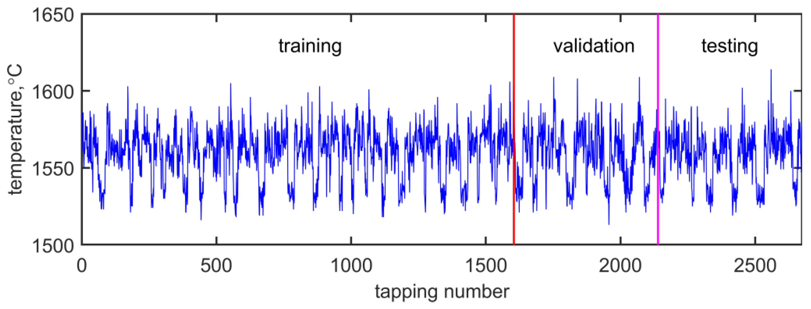
Of the data, about 60% (1604 sets) were used for training, about 20% (535 sets) were used for validation, and the remaining 20% were used for testing. Figure 4 illustrates the evolution of the end temperature of liquid steel in the VTD system. In our experiments, all of the input continuous variables and the output were normalized to the range of [−1, 1]. The goodness of fit of the model was evaluated based on the values of MAE (mean absolute error), MAPE (mean absolute percentage error), RMSE (root-mean-squared error) and the coefficient of determination (R²). The values of the error parameters are calculated as follows (Equations (3)–(6)):

$$MAE=\frac{1}{n}{\sum }_{i=1}^n\left|y_i^a-y_i^p\right|$$

(3)

$$MAPE=\frac{1}{n}{\sum }_{i=1}^n\left|\frac{y_i^a-y_i^p}{y_i^a}\right|\times 100\%$$

(4)

$$RMSE=\sqrt{\frac{1}{n}{\sum }_{i=1}^n{\left(y_i^a-y_i^p\right)}^2}$$

(5)

$$R^2=1-\left(\frac{{\sum }_{i=1}^n{\left(y_i^a-y_i^p\right)}^2}{{\sum }_{i=1}^n{\left(y_i^a-{\overline{y}}_i^a\right)}^2}\right)$$

(6)

where $y_i^a$ is the actual production value, $y_i^p$ is the predicted value, ${\overline{y}}_i^a$ is the average of the actual values, and n is the size of the data set.

3.2. Model Parameter Selection

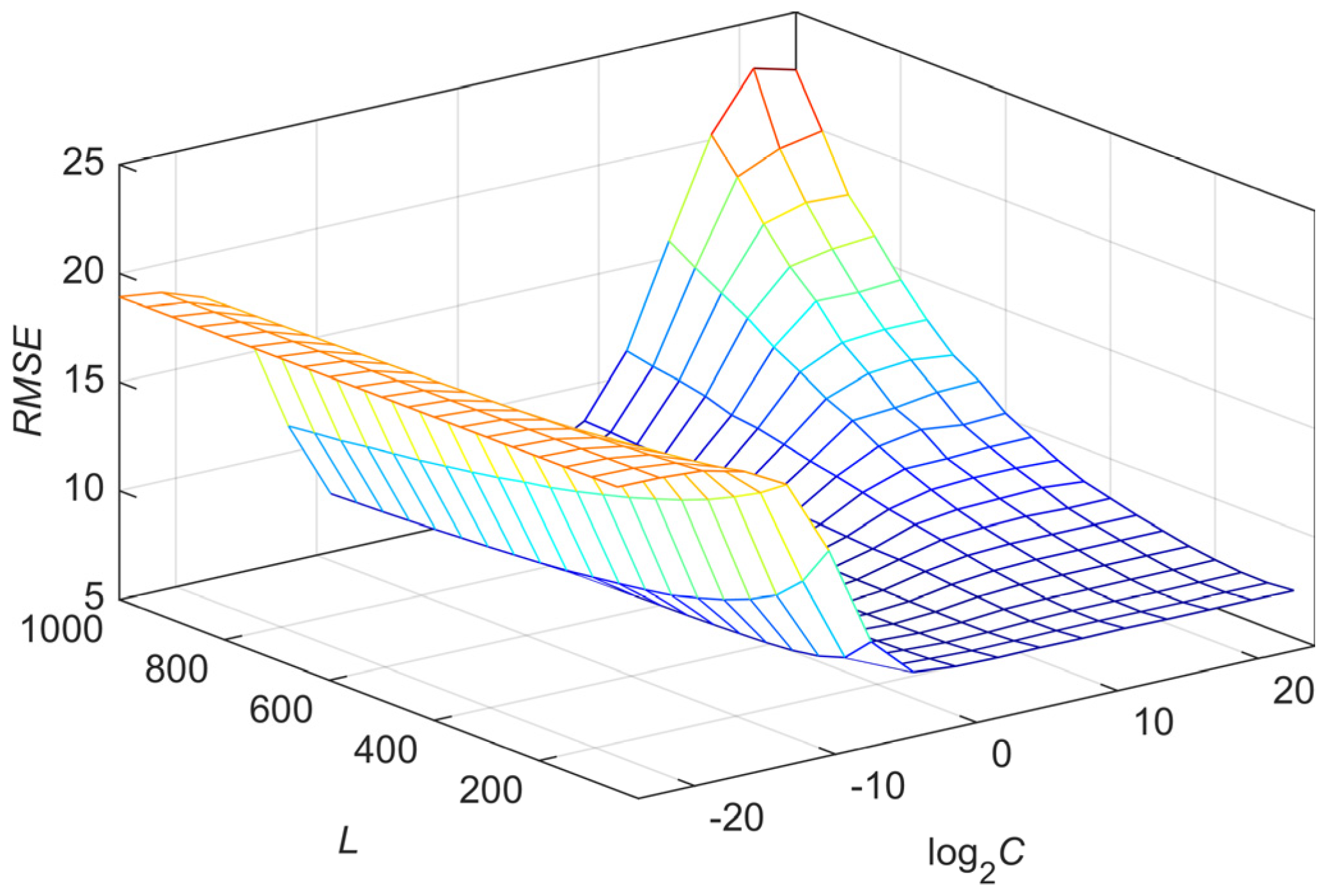
In the proposed prediction model framework, four user-specified parameters are selected to achieve the best generalization performance based on the validation data set. For the ELM network, the sigmoid function G(a, b, x) = 1/(1 + exp(−(a·x + b))) is selected as the activation function. The cost parameter C is selected from the range {2⁻²⁴, 2⁻²³,…, 2²⁴, 2²⁵}, and the number of hidden nodes L is selected from {10, 20,..., 1000}. Thirty trials of simulations were conducted, and the performance of different parameter combinations (C, L) was verified using the average RMSE in the validation set. The parameter combination (C, L) with the smallest RMSE was selected. As seen in Figure 5, ELM can achieve good generalization performance when the cost parameter C is near 2⁰. In other words, the performance of ELM with a sigmoid additive hidden node is not sensitive to the cost parameter C in the range [2⁻⁵, 2¹⁰]. Moreover, C can be specified in a narrow scope.

In addition, for the self-adaptive AdaBoost.RT algorithm, the number of ELMs (T) and the relative factor (λ) need to be determined. In our simulation experiments, the number of ELMs was set to 5, 10, 15, 20, 25 and 30. The relative factor was considered {0.1, 0.2, …, 0.9}. Fifty trials were conducted for each combination of (λ, T).

Table 4. Performance of proposed SAE-ELM model with different values of λ and T.

λ	T
	5	10	15	20	25	30
0.1	6.7786	6.7762	6.7760	6.7747	6.7756	6.7749
0.2	6.7782	6.7762	6.7745	6.7732	6.7738	6.7739
0.3	6.7769	6.7765	6.7765	6.7734	6.7724	6.7741
0.4	6.7747	6.7755	6.7740	6.7741	6.7735	6.7756
0.5	6.7783	6.7756	6.7738	6.7735	6.7733	6.7729
0.6	6.7783	6.7743	6.7746	6.7750	6.7721	6.7743
0.7	6.7795	6.7746	6.7722	6.7742	6.7737	6.7696
0.8	6.7846	6.7747	6.7742	6.7744	6.7729	6.7728
0.9	6.7907	6.7782	6.7785	6.7734	6.7757	6.7747

shows the generalization performance of the validation set with different combinations of (λ, T). As revealed in Table 4, the proposed ensemble ELM-based self-adaptive AdaBoost.RT could achieve good generalization performance on the validation set and is not sensitive to the different values of λ and T. The RMSE has the smallest value when λ = 0.7 and T = 30. Hence, the parameter combination of (λ, T) was chosen as (0.7, 30) in our ensemble predictive model.

3.3. Results and Discussion

Based on the user-specified parameters selected according to the validation data set, the predictive ability of the proposed model was evaluated on the test data set. Fifty trials of simulations were conducted on the test data set, and the average serves as the “final result”. The performance of the proposed model on different data sets is tabulated in

Table 5. Evaluation of the predictive performance of the proposed model.

	Training	Validation	Testing
MAE	4.1081 ± 0.0033	5.3047 ± 0.0082	5.2780 ± 0.0073
MAPE	0.0012 ± 2.2 × 10−6	0.0592 ± 0.0008	0.1295 ± 0.0006
RMSE	5.2511 ± 0.0034	6.7721 ± 0.0098	6.7285 ± 0.0078
R2	0.9021 ± 0.0001	0.8643 ± 0.0004	0.8504 ± 0.0003

. As shown in Table 5, the MAE, MAPE, RMSE and R² of the training set are the smallest among the three different data sets. This indicates that the model is well trained and can be applied to establish the end-temperature prediction model. The R² between the actual production values and predicted values is about 0.90 for the training of the ensemble model, which indicates that 90% of the variation in the end temperature could be explained using the proposed model. For the validation and testing of the predictive model, the calculated values of R² are higher than 0.85, which indicates the adequacy of the model developed for predicting the end temperature of liquid steel in the VTD refining process.

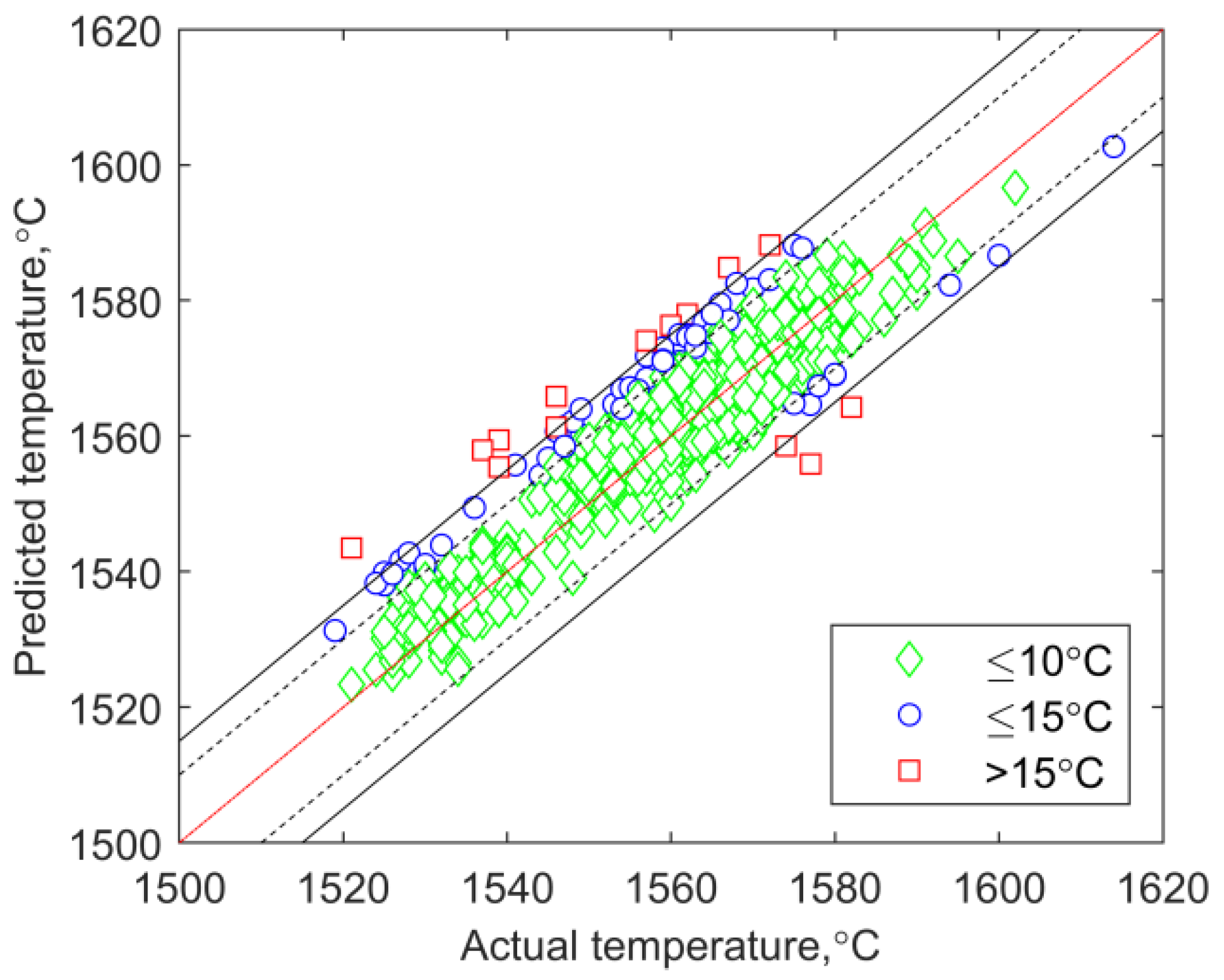
The actual measurements versus model predictions of the test data set are presented in Figure 6. Figure 6 shows the prediction results of the 535 test temperature points according to the actual value. The green diamonds indicate that the absolute error between the predicted and actual temperatures is lower than 10 °C. The blue circles denote an absolute error between 10 °C and 15 °C. The red squares denote an absolute error larger than 15 °C. The results achieved with the predictive model are a 91.02% accuracy for an absolute error under 10 °C and a 98.35% accuracy for a relative tolerance of 15 °C. This indicates the consistent and high concurrence of the predicted values with the actual values. Actually, the sensitivity and robustness of the ensemble model to predict the temperature drop in liquid steel with excellent accuracy were achieved. The predicted results are in good agreement with the actual data with <1.7% error.

For comparison, the single ELM model [30], the original AdaBoost.RT [26] and robust AdaBoost.RT [28] were tested in experiments. The parameters (C, L) for single ELM and other ELM-based ensemble methods were selected to be the same as in our proposed method. The threshold value for the original AdaBoost.RT was selected from the range {0.1, 0.15, …, 0.4}. The best threshold value with the smallest RMSE on the validation set after thirty trials was selected. Fifty trials of simulations were conducted on the test data set. The test results of comparisons between our proposed self-adaptive AdaBoost.RT and other learning algorithms are shown in

Table 6. Comparison of test performance of different models.

Model	MAE	MAPE	RMSE	R2
Single ELM [30]	5.2948 ± 0.0269	0.1298 ± 0.0022	6.7492 ± 0.0314	0.8495 ± 0.0014
AdaBoost.RT [26]	5.2785 ± 0.0077	0.1295 ± 0.0007	6.7283 ± 0.0087	0.8504 ± 0.0004
Robust AdaBoost.RT [28]	5.2778 ± 0.0082	0.1294 ± 0.0007	6.7291 ± 0.0091	0.8503 ± 0.0004
Proposed method	5.2780 ± 0.0073	0.1295 ± 0.0006	6.7285 ± 0.0078	0.8504 ± 0.0003

. The accuracy reached by the proposed ELM-based self-adaptive AdaBoost.RT intelligent modeling technique is much higher compared with the previous regression methods. Here, it should be pointed out that the proposed model obtained the best generalization performance among the four algorithms. The improvement in the temperature drop prediction is significant using the ensemble technique and could be increased by precisely selecting the threshold value in the AdaBoost.RT algorithm.

4. Application

The end temperature of liquid steel during the vacuum degassing process depends on many parameters, such as the initial temperature of liquid steel in VTD, the refining process conditions of vacuum degassing (vacuum arrival time, refining time, vacuum holding time, soft stirring time and argon consumption), liquid steel status (liquid steel weight) and other process parameters (tap-to-VTD time).

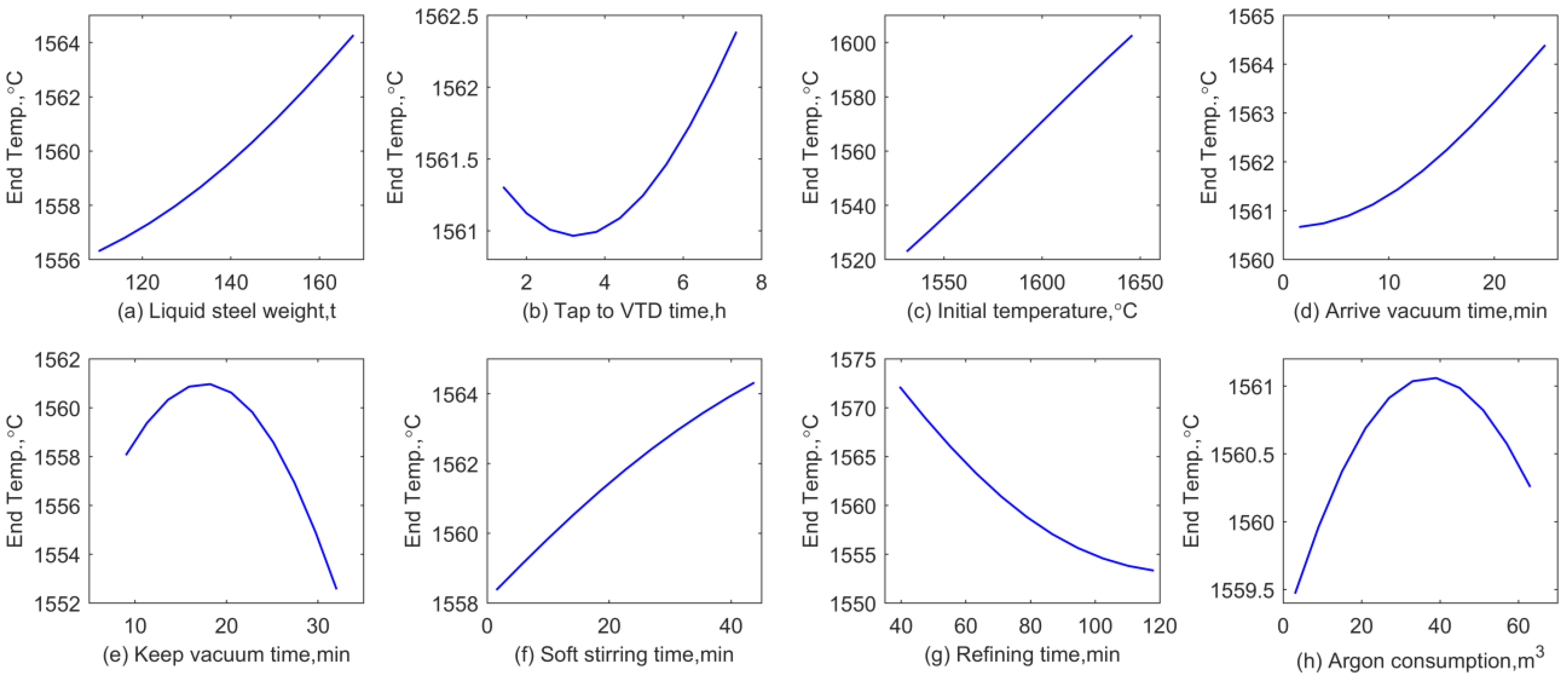
The single-factor method was applied to determine the influence of each factor on the end temperature of liquid steel. The method is as follows: when analyzing the influence of factor i on the target, factor i is taken as an equal-difference sequence in its range, and all other input parameters are taken as an average value. Then, these data are normalized and input into the trained model as a sample matrix to obtain the output value of the index. A sensitivity analysis of parameters was carried out to understand their effects on the end temperature. The results are shown in Figure 7.

Liquid steel is the main carrier of heat in the ladle furnace. The greater the weight of liquid steel, the more total heat it contains, and the less heat loss in the VTD system. This results in the end temperature increasing with the increase in the weight of liquid steel (see Figure 7a for the effect of liquid steel weight on the end temperature).

The tap-to-VTD time is the time before the ladle furnace arrives at VTD, and its effect on the end temperature is depicted in Figure 7b. The relationship between the tap-to-VTD time and the end temperature is a quadratic curve. However, the absolute influence value is small, and the maximum temperature error is less than 2 °C.

The initial temperature represents the initial state of liquid steel in the ladle furnace. Figure 7c shows the influence of the initial temperature on the end temperature. The higher the initial temperature, the higher the end temperature.

The vacuum arrival time is the time when the pressure in the VTD drops from atmospheric pressure to a very low operating pressure (i.e., 67 Pa) inside the chamber. The effect of the vacuum arrival time on the end temperature is depicted in Figure 7d. The vacuum holding time (Figure 7e) governs the main vacuum degassing process as well as the soft stirring time (Figure 7f). The main purpose of soft stirring is to move inclusions into the slag layer to improve the purity of refined steel, and the other purpose is to precisely control the temperature of cast-in-place casting. Soft stirring makes the temperature of the liquid steel uniform in the ladle furnace and reduces the temperature drop during the vacuum degassing process. The refining time represents the residence time of the ladle furnace in the vacuum chamber. A longer residence time leads to more heat loss and results in a higher temperature drop. Thus, the longer the refining time, the lower the end temperature, as shown in Figure 7g.

Argon gas is blown into the ladle furnace to stir liquid steel and to refine steel under a vacuum and an inert gas protection environment. As shown in Figure 7h, the relationship between the argon gas consumption and the end temperature of liquid steel presents a quadratic curve function.

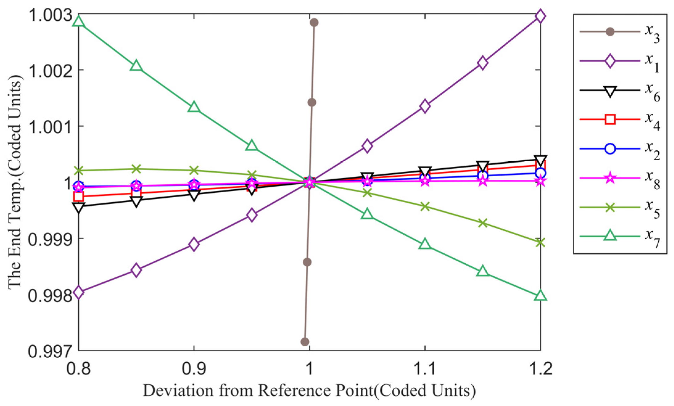
To check the significance of the effects of the operating parameters on the end temperature, a sensitivity analysis of the factors was carried out on the data obtained, as shown in Figure 8. Figure 8 shows a perturbation plot illustrating the influence of single independent variables on the end temperature. It can be seen that the end temperature increases with the initial temperature (x₃) more drastically than other operating parameters, and the relationship between the initial temperature and end temperature is approximately linear. In other words, the end temperature increases proportionally to the initial temperature. The value of the end temperature increases as the weight of liquid steel increases in the design range. The effect of the weight of liquid steel on the end temperature in the right region of the design center point is greater than in the left region. The end temperature decreases as the refining time increases in the design range. This phenomenon is due to heat dissipation during the vacuum degassing process. Compared with the later stage of the design center point, heat dissipation is faster in the early stage. The vacuum holding time is the fourth influencing factor of the eight variables, and the effect on the end temperature in the right region of the design center point is greater than in the left region. The effects of the other four parameters on the end temperature are not obvious according to the previous four operating factors.

To obtain the polynomial calculation equation of the end temperature, a stepwise regression method was carried out on the operating parameters and quadratic factors, which were constructed according to the sensitivity analysis of the single parameters. Equation (7) is the stepwise regression result based on the training data set. From Equation (7), it can be seen that the ladle material is the most important factor among the three discrete factors, and the end temperature decreases as the numerical value of the ladle material increases.

Y_end = 0.74x₃ + 1.80x₅ + 0.18x₆ − 0.80x₇ + 0.27x₈ − 2.59x₉ + 0.0005x₁² + 0.048x₂² + 0.0097x₄² − 0.0506x₅² + 0.0031x₇² − 0.0034x₈² + 396.45

(7)

Further, the polynomial calculation equation was applied to the validation and test sets of the ladle furnaces in the VTD system to verify its effectiveness.

Table 7. Prediction performance of polynomial calculation equation.

Data Sets	MAE	MAPE	RMSE	R2
Training	4.5826	0.2940	5.8843	0.8770
Validation	5.5871	0.3591	7.1188	0.8522
Testing	5.4523	0.3503	6.8864	0.8409

shows the predictive performance of Equation (7) on the different production data sets. In the last row of Table 7, R² is the coefficient of determination to represent the proportion of the variance in the response variable that is predictable from the independent variables. An R² value of 0.8409 on the test data set indicates a high correlation between the actual end temperature and predicted results. Both the training R² and the validation R² are larger than 0.85, indicating that the equation has a good generalization ability. The adequate precision in Table 7 represents the polynomial calculation equation efficiency for predicting the end temperature of liquid steel in the VTD system.

Since control would be the ultimate goal and VTD control often means controlling the temperature and components of liquid steel, the current prediction model can better serve control purposes. A self-adaptive threshold was created to replace the constant threshold in the original AdaBoost.RT algorithm. In prediction applications, the ELM predictor and the self-adaptive AdaBoost.RT algorithm are adopted to predict the end temperature. Another contribution made in this study is the development of an exact formula to calculate the end temperature. Since it is not easy to select the nonlinear terms of independent variables, black-box modeling techniques still form the main basis for performing VTD control today. For this reason, the current work has tried to address the VTD control problem through a polynomial calculation equation from the VTD black-box SAE-ELM model using a stepwise regression method. Therefore, the novelty of this study is the presentation of a new strategy to obtain a possible solution to the VTD issue, in which the discrete ladle status is first transformed into numerical codes; then, self-adaptive AdaBoost.RT ensemble ELMs are used to perform the prediction task; finally, a polynomial calculation equation is established from the SAE-ELM black-box model through a stepwise regression method to find the solution to the end-temperature control problem.

From the viewpoint of developing VTD models, the proposed strategy renders a novel model that can take advantage of VTD black-box models to generate features. The main motivation driving the current study is that the operation of a VTD is still a serious problem in practice. Although plenty of research on the modeling and control of a VTD system has been conducted in the past few decades, the experience of skilled operators is still the main driver for a smooth operation. In addition, the paramount importance of clean steel in the national economy makes research on VTD system modeling and control still very active in the foreseeable future. Hence, the proposed model is still significant and makes a slight improvement to the VTD system.

5. Conclusions

• An ensemble model for predicting the end temperature of liquid steel in VTD has been presented. The parameters influencing the end temperature of liquid steel in VTD are determined by analyzing the actual refining process and energy equilibrium of VTD. A numeric encoding method is introduced to switch the discrete variables (ladle conditions) to numeric codes. The effect of the process factors on the end temperature in VTD is modeled using an ensemble approach based on self-adaptive AdaBoost.RT combined with ELM. The self-adaptive AdaBoost.RT algorithm is proposed by using the statistical distribution of a weak learner’s predictions to dynamically determine the threshold of the relative error.
• Adopting the ensemble model, we can construct the end-temperature prediction model with an accuracy of 91.02% for an absolute error under 10 °C. The proposed ensemble model has the ability to successfully predict the values, which demonstrates the potential for the reliable prediction of the end temperature of liquid steel in VTD. The developed model can act as a potential tool for predicting the end temperature in advance, which will be helpful in precisely controlling the process of VTD.
• The modified self-adaptive AdaBoost.RT algorithm can be applied to solve the regression problem. The method of coupling continuous and discrete variables can be applied to analyze the influence of input factors on the target output indexes, especially when there are complex parameters in the system.
• The self-adaptive AdaBoost.RT algorithm can improve the performance of regression models using previous approaches. The absolute relative error is used to define the error rate in the AdaBoost.RT algorithm. Hence, the output value y_i should not be 0, and the average value of predictions μ should not be 0 in our proposed self-adaptive AdaBoost.RT algorithm. The proposed hybrid prediction frameworks can be programmed and validated conveniently on the Matlab platform.

References

1. Morshed-Behbahani, K.; Zakerin, N. A review on the role of surface nanocrystallization in corrosion of stainless steel. J. Mater. Res. Technol. 2022, 19, 1120–1147. [Google Scholar] [CrossRef]
2. Mohammadzehi, S.; Mirzadeh, H. Cold unidirectional/cross-rolling of austenitic stainless steels: A review. Arch. Civ. Mech. Eng. 2022, 22, 129. [Google Scholar] [CrossRef]
3. Sun, J.; Tang, H.; Wang, C.; Han, Z.; Li, S. Effects of alloying elements and microstructure on stainless steel corrosion: A review. Steel Res. Int. 2022, 93, 2100450. [Google Scholar] [CrossRef]
4. Romero-Resendiz, L.; El-Tahawy, M.; Zhang, T.; Rossi, M.C.; Marulanda-Cardona, D.M.; Yang, T.; Amigó-Borrás, V.; Huang, Y.; Mirzadeh, H.; Beyerlein, I.J.; et al. Heterostructured stainless steel: Properties, current trends, and future perspectives. Mater. Sci. Eng. R 2022, 150, 100691. [Google Scholar] [CrossRef]
5. Ghayoor, M.; Mirzababaei, S.; Sittiho, A.; Charit, I.; Paul, B.K.; Pasebani, S. Thermal stability of additively manufactured austenitic 304L ODS alloy. J. Mater. Sci. Technol. 2021, 83, 208. [Google Scholar] [CrossRef]
6. Silva, A.M.B.; Peixoto, J.J.M.; da Silva, C.A.; Silva, I.A. Steel desulfurization on RH degasser: Physical and mathematical modeling. Metall. Mater. 2022, 75, 27. [Google Scholar] [CrossRef]
7. Kumar, N.; Yadav, A.S.; Chaudhari, G.P.; Meka, S.R. Effect of severe plastic deformation on pre- and post-nitriding conditions of 316 stainless steel. Trans. Indian Inst. Met. 2022, 75, 2787. [Google Scholar] [CrossRef]
8. Li, Y.; Zhu, H.; Wang, R.; Ren, Z.; Lin, L. Prediction of two phase flow behavior and mixing degree of liquid steel under reduced pressure. Vacuum 2021, 192, 110480. [Google Scholar] [CrossRef]
9. Tang, D.; Pistorius, P.C. Kinetics of nitrogen removal from liquid third generation advanced high-strength steel by tank degassing. Metall. Mater. Trans. B 2022, 53B, 1383. [Google Scholar] [CrossRef]
10. Da Rocha, V.C.; Pereira, J.A.M.; Yoshioka, A.; Bielefeldt, W.V.; Vilela, A.C.F. Effective viscosity of slag and kinetic stirring parameter applied in steel cleanliness during vacuum degassing. Mater. Res. 2017, 20, 1480. [Google Scholar] [CrossRef]
11. Pylvänäinen, M.; Visuri, V.V.; Nissilä, J.; Laurila, J.; Karioja, K.; Ollila, S.; Liedes, T. Vibration-based monitoring of gas-stirring intensity in vacuum tank degassing. Steel Res. Int. 2020, 91, 10. [Google Scholar] [CrossRef]
12. Thapliyal, V.; Lekakh, S.N.; Peaslee, K.D.; Robertson, D.G.C. Novel modeling concept for vacuum tank degassing. In Proceedings of the 2012 AISTech, The Iron & Steel Technology Conference and Exposition, Atlanta, GA, USA; Warrendale, PA, USA, 7–10 May 2012; p. 1143. [Google Scholar]
13. Yu, S.; Louhenkilpi, S. Numerical simulation of dehydrogenation of liquid steel in the vacuum tank degasser. Metall. Mater. Trans. B 2013, 44, 459. [Google Scholar] [CrossRef]
14. Yu, S.; Miettinen, J.; Shao, L.; Louhenkilpi, S. Mathematical modeling of nitrogen removal from the vacuum tank degasser. Steel Res. Int. 2015, 86, 466. [Google Scholar] [CrossRef]
15. Khan, M.; Lao, J.; Dai, J.-G. Comparative study of advanced computational techniques for estimating the compressive strength of UHPC. J. Asian Concr. Fed. 2022, 8, 51. [Google Scholar] [CrossRef]
16. Gajic, D.; Savic-Gajic, I.; Savic, I.; Georgieva, O.; Di Gennaro, S. Modelling of electrical energy consumption in an electric arc furnace using artificial neural networks. Energy 2016, 108, 132. [Google Scholar] [CrossRef]
17. Kordos, M.; Blachnik, M.; Wieczorek, T. Temperature prediction in electric arc furnace with neural network tree. In Artificial Neural Networks and Machine Learning ICANN; Springer: Berlin/Heidelberg, Germany, 2011; p. 71. [Google Scholar]
18. Fernndez, J.M.M.; Cabal, V.A.; Montequin, V.R.; Balsera, J.V. Online estimation of electric arc furnace tap temperature by using fuzzy neural networks. Eng. Appl. Artif. Intell. 2008, 21, 1001. [Google Scholar] [CrossRef]
19. Rajesh, N.; Khare, M.R.; Pabi, S.K. Feed forward neural network for prediction of end blow oxygen in LD converter steel making. Mater. Res. 2010, 13, 15. [Google Scholar] [CrossRef] [Green Version]
20. Wang, X.; You, M.; Mao, Z.; Yuan, P. Tree-structure ensemble general regression neural networks applied to predict the molten steel temperature in ladle furnace. Adv. Eng. Inform. 2016, 30, 368. [Google Scholar] [CrossRef]
21. Wang, S.; Li, H.; Zhang, Y.; Zou, Z. An integrated methodology for rule extraction from ELM-based vacuum tank degasser multiclassifier for decision-making. Energies 2019, 12, 3535. [Google Scholar] [CrossRef] [Green Version]
22. Su, H.; Yu, Y.; Du, Q.; Du, P. Ensemble learning for hyperspectral image classification using tangent collaborative representation. IEEE Trans. Geosci. Remote Sens. 2020, 58, 3778. [Google Scholar] [CrossRef]
23. Mosca, A.; Magoulas, G.D. Customised ensemble methodologies for deep learning: Boosted residual networks and related approaches. Neural Comput. Appl. 2019, 31, 1713. [Google Scholar] [CrossRef] [Green Version]
24. Drucker, H. Improving regressors using boosting techniques. In Fourteenth International Conference on Machine Learning; Morgan Kaufmann Publishers Inc.: Burlington, MA, USA, 1997; p. 107. [Google Scholar]
25. Solomatine, D.L.; Shrestha, D.L. AdaBoost. RT: A boosting algorithm for regression problems. Neural Netw. 2004, 2, 1163. [Google Scholar]
26. Shrestha, D.L.; Solomatine, D.P. Experiments with AdaBoost.RT, an improved boosting scheme for regression. Neural Comput. 2006, 18, 1678. [Google Scholar] [CrossRef] [PubMed]
27. Tian, H.-X.; Mao, Z.-Z. An ensemble ELM based on modified AdaBoost.RT algorithm for predicting the temperature of molten steel in ladle furnace. IEEE Trans. Autom. Sci. Eng. 2009, 7, 73. [Google Scholar] [CrossRef]
28. Zhang, P.-B.; Yang, Z.-X. A novel AdaBoost framework with robust threshold and structural optimization. IEEE Trans. Cybern. 2016, 48, 64. [Google Scholar] [CrossRef]
29. Lichman, M. UCI Machine Learning Repository; School of Information and Computer Science, University of California: Irvine, CA, USA, 2013; Available online: http://archive.ics.uci.edu/mL (accessed on 6 May 2019).
30. Huang, G.-B.; Zhou, H.; Ding, X.; Zhang, R. Extreme learning machine for regression and multiclass classification. IEEE Trans. Syst. Man Cybern. Part B 2012, 42, 513. [Google Scholar] [CrossRef] [Green Version]
31. Liu, X.; Gao, C.; Li, P. A comparative analysis of support vector machines and extreme learning machines. Neural Netw. 2012, 33, 58. [Google Scholar] [CrossRef]
32. Wang, S.H.; Li, H.F.; Zhang, Y.J.; Zou, Z.S. A hybrid ensemble model based on ELM and improved AdaBoost. RT algorithm for predicting the iron ore sintering characters. Comput. Intell. Neurosci. 2019, 2019, 4164296. [Google Scholar] [CrossRef] [Green Version]
33. Zhang, X.-L.; Liu, P. A new delay jitter smoothing algorithm based on Pareto distribution in Cyber-Physical Systems. Wirel. Netw. 2015, 21, 1913. [Google Scholar] [CrossRef]
Figure 1. Process flow diagram of VTD.
Metals 12 02028 g001
Figure 2. The energy conservation of VTD (Qsurf, heat loss from the top surface; Qargon, heat loss due to argon stirring; Qgas, heat loss of the gas used during vacuumizing and vacuum breaking; Qladle, heat content absorbed by ladle lining; Qshell, convection loss to atmosphere from ladle shell).
Metals 12 02028 g002
Figure 3. Ensemble ELM model based on self-adaptive AdaBoost.RT algorithm.
Metals 12 02028 g003
Figure 4. Evolution of the end temperature of liquid steel in VTD system.
Metals 12 02028 g004
Figure 5. The average validation RMSE with different values of C and L.
Metals 12 02028 g005
Figure 6. Residual graph of end temperature between actual and predicted values.
Metals 12 02028 g006
Figure 7. Sensitivity analysis of variables on the end temperature of liquid steel in VTD. The influencing factors are listed as (a) liquid steel weight, (b) tap to VTD time, (c) initial temperature, (d) arrive vacuum time, (e) keep vacuum time, (f) soft stirring time, (g) refining time, (h) argon consumption.
Metals 12 02028 g007
Figure 8. The perturbation plot illustrating the influence of single independent variables on the end temperature.
Metals 12 02028 g008