Article

Improved SVM Model for Predicting Pellet Metallurgical Properties Based on Textural Characteristics

1
Hebei Engineering Research Center for the Intelligentization of Iron Ore Optimization and Ironmaking Raw Materials Preparation Processes, North China University of Science and Technology, Tangshan 063210, China
2
Tangshan Intelligent Industry and Image Processing Technology Innovation Center, North China University of Science and Technology, Tangshan 063210, China
3
College of Metallurgy and Energy, North China University of Science and Technology, Tangshan 063210, China
*
Author to whom correspondence should be addressed.
Metals 2022, 12(10), 1662; https://doi.org/10.3390/met12101662
Submission received: 6 July 2022 / Revised: 25 August 2022 / Accepted: 20 September 2022 / Published: 2 October 2022
(This article belongs to the Special Issue Big Data of Steel and Low Carbon Intelligent Smelting)

Abstract

:
From the point of view that pellet microstructure determines its metallurgical properties, an improved support vector machine (SVM) model for pellet metallurgical properties forecast is studied based on the mineral phase characteristics, in order to improve the evaluation efficiency of pellet metallurgical properties. The forecast model is composed of a SVM with self-adaptive selection of kernel parameters and a SVM with self-adaptive compounding of kernel types. This not only guarantees the super interpolation ability of the forecast model, but also takes into account its good generalization performance. Based on 200 sets of original sample information, the quantitative relationship between the main characteristics of mineral phase and the grade labels of pellet metallurgical properties (reduction expansion index RSI, reduction index RI, low temperature reduction and pulverization index RDI) was determined by the improved SVM model. With the simulation results of RSI, RI, and RDI with the accuracy of 100%, 98%, and 100% respectively, the precise forecast of pellet metallurgical properties based on mineral phase is realized.

1. Introduction

During the “13th Five-Year Plan” period, the steel industry’s development goals are targeted at: resolving excess capacity, carrying out large-scale structural restructuring, curbing disorderly competition in the industry, increasing product innovation, promoting green development, and encouraging enterprises to go global. In this context, the whole steel industry is facing a severe test. As a necessary raw material, the metallurgical properties of pellets directly affect the quality of the molten iron and the smooth running of the blast furnace. However, there are many indicators to evaluate the metallurgical properties of pellets, the quality inspection process is complicated. and the cost of consumables is large [1,2,3,4,5].
Based on the objectives of “increasing product innovation” and “promoting green development”, some scholars have analyzed the mineral phases and further related the mineral phases to the metallurgical properties of pellets [6,7,8,9]. From the importance of pellet microstructure, the mineral phases of pellets are analyzed. There is no doubt about the theoretical feasibility of this perspective. However, the determination and analysis of mineral phases by scholars at home and abroad are mostly at the stage of manual experience, and there are few studies on extracting the characteristics of mineral phases with the help of image graphic processing algorithms. Therefore, it is necessary to explore an efficient pellet metallurgical performance prediction algorithm based on the ore phase.
Support vector machines (SVM), based on statistical learning theory and machine learning theory, have a solid mathematical theoretical foundation compared with existing learning machines, and have strong generalization and nonlinear processing capabilities, especially when dealing with high-dimensional data, without having to map it to higher dimensions, which can well avoid “dimensional disasters” [10,11,12]. The key technique for SVM to deal with non-linear data sets is the kernel function, and different kinds of kernel functions or kernel functions with different parameters will cause changes in the feature space, i.e., the reasonable selection of kernel types and kernel parameters is the key to the performance of SVM models. The key aspect of SVM improvement lies in the kernel function, and the direction of improvement is broadly divided into two categories: optimal selection of the kernel function type and optimal selection of the kernel function parameters [13,14,15,16]. It is a good choice to study a more superior SVM improvement model for pellet metallurgical performance prediction if the selection of SVM kernel parameters and the selection of SVM kernel types can be considered comprehensively. Based on this, this study comprehensively considers the two directions of SVM kernel function improvement and designs a coupling model of the adaptive selection of kernel parameters and adaptive combination of kernel species, then applies the model to the prediction of metallurgical properties of pellets, in order to obtain good results.

2. Construction of the Sample Set

In order to explore the relationship between pellet phases and their metallurgical properties, a total of 200 sets of pellet samples with their corresponding metallurgical properties were collected, and the 200 sets of experimental data were assigned sample numbers 1~200. The sample set consists of two parts, input and output, and the two sections of this chapter focus on demonstrating the rationality and scientificity of the sample set construction.

2.1. Extraction of Pellet Phase Characteristics

The original SEM images of the central part, one quarter part, and edge part of the pellet sample were labeled with sample number i (i = 1, 2,…, 200), and the corresponding [Al], [Ca], the coloring and labeling images of seven elements [C], [Fe], [Mg], [O], and [Si], i.e., each group of samples is used as the input image for a total of 24 images, and the 24 images are named. In order to reduce the complexity of the algorithm and improve the quality of the pellet metallurgical performance prediction sample set, the main texture features of the 200 groups of 4800 pellets were extracted.
Texture features of digital images do not depend on image color and image brightness, but only on the result of color contrast and brightness contrast. Based on the threshold setting, the internal change pattern and characteristics of the image are detected according to the sequence characteristics and structural characteristics of the image, and the contents that match the visual effect are extracted. These contents are used as texture features of digital images to be applied to the actual image detection and recognition problems.
The grayscale co-occurrence matrix algorithm is a method to describe image texture information based on the probability of recurrence of a certain gray level structure in an image, based on probabilistic information, the method of probability adjustment is studied to clarify the grayscale image texture structure. Let the total number of pixels in the x-axis direction be Nx and the total number of pixels in the y-axis direction be Ny. In order to avoid the huge computational effort caused by analyzing numerous grey levels, the image grey levels are grouped together, and G denotes the number of grey levels after grouping, whose highest grey level is the Ngth level.
The grayscale co-occurrence matrix of an image reflects the comprehensive information of the image grayscale about direction, adjacent interval and change magnitude, which is the basis for analyzing the local patterns and alignment rules of the image.
Once the grey co-generation matrix in each of the four directions has been determined, the following texture eigenvalues defined by the grey co-generation matrix algorithm need to be calculated separately, and finally the mean of the various eigenvalues is used as each component in the texture vector [17]. The texture feature vector of an image consists of a series of eigenvalues, including: angular second order moment (UNI), contrast (CON), correlation (COR), entropy (ENT), difference (VAR), inverse disparity (IDM), sum average (SA), sum variance (SD), sum entropy (SENT), variance difference (DV), difference entropy (DE), mutual information metric (IMC), maximum correlation coefficient (MCC), maximum probability (MAX), dissimilarity (DIS), inverse variance (INV), median, homogeneity, cluster shade, and cluster prominence. Among the above 20 eigenvalues, the angular second-order moment UNI and contrast CON are the most effective for texture discrimination from a single eigenvalue.
The pellet phase texture feature extraction process is shown in Figure 1:

2.2. Integration of Sample Sets

The total number of samples is 200 and the number of images used as input is 24 × 200.
Output: Grade label for metallurgical properties of pellet (reduction expansion index, reduction index, low temperature reduction pulverization properties).
The reduction swelling index is a low superior indicator, whereas the reduction index and low temperature reduction chalking index are high superior indicators. The Chinese national standard (GB/T13242-91) test method was used after the reduction of the specimen through the N2 cooling, before loading into a small drum (ϕ 130 mm × 200 mm), at 30 r/min rotation speed for 10 min, the drum after the specimen for sieving, to +6.3 mm, +3.15 mm, −0.5 mm particle size of the mass. The percentage of the ratio of the mass of +6.3 mm, +3.15 mm, and −0.5 mm to the total mass of the reduced specimens in the drum was used as the reduction chalking index. The RDI+3.15 is used as the assessment index, while the RDI+6.3 and RDI−0.5 are only used as reference indicators.
The reduction swelling index grade 1 was labelled 001, grade 2 was labelled 010, and grade 3 was labelled 100. The reduction degree index grade 1 was labelled +1, grade 2 was labelled 0, and grade 3 was labelled −1. The low temperature reduction chalking index grade 1 was labelled 01, grade 2 was labelled 02, and grade 3 was labelled 03. The sample input was then explored separately in relation to the reduction swelling index, reduction degree index, and low temperature reduction chalking index grade labels. Since the relationships between the mineral phase and the three index grade labels of metallurgical properties were explored separately, three sample sets were constructed and the initial sample set structure is shown in Figure 2.
The extracted sample sets were constructed with the sample input being the main features of the ore phase texture and the output being the grade labels of the metallurgical properties of the pellet. The extracted five main features of ore phase texture were used as sample inputs, and the grade labels of reduction swelling index, reduction degree index, and low temperature reduction pulverization index were used as sample outputs, respectively (Table 1).

3. Predictive Modeling of Pellet Metallurgical Properties

3.1. Related Knowledge

There are three types of data samples collected based on support vector classification, one of which is linearly divisible, the other is linearly incompletely divisible, and the third is linearly indivisible [18,19]. For linearly divisible samples, the optimal classification hyperplane can be obtained directly by using the maximum interval theory. For linearly incompletely divisible samples, the relaxation variable si and the penalty parameter C need to be introduced on the basis of the linearly divisible optimization function to restrict the misclassification. For linearly inseparable samples, finally obtain the optimal classification hyperplane in the linearly indivisible case. For linearly indistinguishable samples, it is necessary to map the initial linearly indistinguishable samples into a higher dimensional feature space with the help of the kernel function Φ(x). The classification hyperplane that can achieve linearly divisible samples is searched for in the high-dimensional feature space, and the optimal classification hyperplane is locked in the SVM solving framework with the equivalent mapping of the kernel function for nonlinear problems (see Figure 3).
The kernel function can be expressed as the inner product of two vectors in a certain feature space, see Equation (1):
K ( x i , x j ) = Φ ( x i ) , Φ ( x j )
The inner product of the original sample space point and the corresponding high-dimensional sample space point can obtain the distribution characteristics of the sample point in the high-dimensional feature space. Since the realization of sample classification only needs to clarify the characteristics of the sample point in the high-dimensional space, there is no need to analyze the coordinates determined in the high-dimensional space. point. In actual operation, by adjusting the form of the kernel function, the change of the high-dimensional space mapping feature can be realized, i.e., the introduction of the kernel function will not increase the complexity of the algorithm implementation and avoid the “dimension disaster”. This means that the introduction of kernel functions does not increase the complexity of the implementation of the algorithm and avoids the “dimensional disaster”. In this paper, three typical kernel functions for SVM are studied: the RBF kernel, the polynomial kernel and the Sigmoid kernel.
(1) The RBF (radial basis function) kernel is most widely used in practice for its superb interpolation performance. The kernel function has only one kernel parameter called the kernel radius σ. The RBF kernel maps the original space samples onto the high-dimensional space in an implicit form, reflecting a high-dimensional space dimension of ∞, corresponding to the image of the original space sample points is not a specific infinite dimension, but only a sub-popularity of the feature space, and the SVM framework under The RBF kernel mapping reflects a sample dimension that does not exceed the original sample dimension at most. In the practical application of SVM, lacking a priori knowledge of the sample data under study, good results are always achieved using the RBF kernel function as long as the parameters are chosen appropriately. The excellent nature of the RBF kernel function determines the superb local learning capability of the RBF kernel SVM, although overlearning is still unavoidable in practical applications.
(2) The polynomial kernel function is also a very common kernel function, which has only one integer kernel parameter q. The polynomial kernel shows significant advantages at long range points, but the accuracy at close range points is not high, which is due to the fact that the kernel function focuses more on the global information of the sample, weakening its interpolation ability and enhancing its generalization ability.
(3) The Sigmoid kernel prototype is a neural network learning function that is equivalent to a bilayer neural network in the SVM framework. The Sigmoid kernel function has two kernel parameters, γ and c, whose kernel matrix is not semi-positive definite for some values. First, the Sigmoid kernel is conditionally positive definite for some values of γ and c. Then, for the kernel function corresponding to the SVM, conditional positive definiteness is sufficient. Both the Sigmoid kernel and the polynomial kernel are global kernel functions that satisfy the characteristic of weak local interpolation and strong global generalization.
Theoretical analysis shows that the SVM kernel function is not necessarily a positive definite kernel, and that corrections to non-positive kernels can also be applied in the SVM framework. The kernel matrix can be used in the framework of the SVM algorithm as long as it can be processed with the aid of matrix spectra to satisfy positive definiteness. However, there are some shortcomings in the matrix spectrum technique, namely the weak generalization performance, i.e., the inability to accurately apply the classifier to unknown samples, which is limited by the fact that the processed SVM kernel is not guaranteed to remain unchanged in nature.

3.2. Forecasting Model Algorithm Design

The analysis of the properties of three typical kernel functions, namely the RBF kernel function, the polynomial kernel function, and the Sigmoid kernel function, shows that each single kernel function has its own limitations, so the composite kernel function can be constructed by combining two or more kernel functions, which can take into account the advantages of other single kernel functions to obtain a better performance of the SVM. However, if too many single kernel functions are compounded, the resulting composite kernel function will have too many parameters to choose and the performance will be poorer than that of a single kernel function. Therefore, the key issue is how to construct a composite kernel function that is suitable for most problems using as few types of single kernels as possible.
In this study, the RBF kernel function, the polynomial kernel function and the Sigmoid kernel function are compounded as a single kernel function, and the compound kernel function is shown in Equation (2). In Equation (2), the composite weights were optimized during the interaction:
K ( x , y ) = ρ 1 exp ( x y 2 2 σ 2 ) + ρ 2 ( x y + p ) q + ρ 3 tanh ( r x , y + c )
ρ1, ρ2, ρ3 in Equation (2) are composite weights and ρ1 + ρ2 + ρ3 = 1.
The individuals, populations, fitness functions and chromosome codes in the improved design of the SVM algorithm based on the genetic algorithm implementation are shown below.
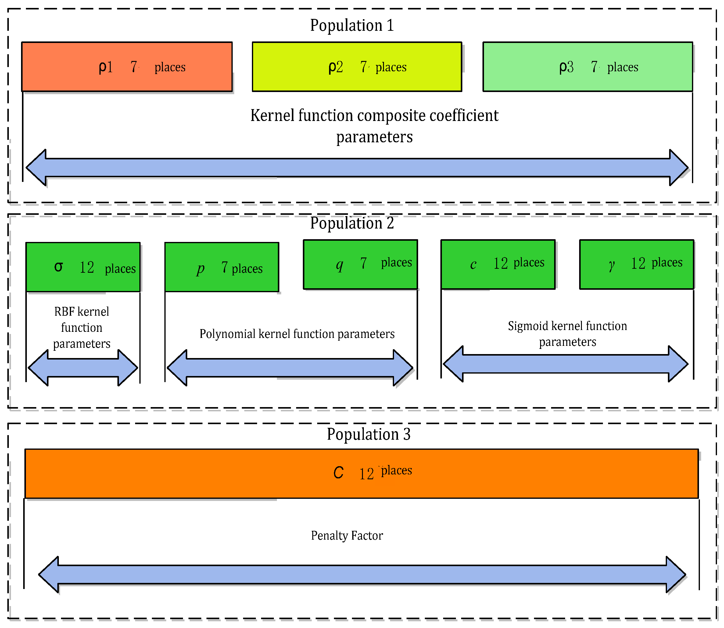
(1) Individual: The individual consists of three kernel function complex coefficients ρ1, ρ2, ρ3 2208 R+, the RBF kernel parameter σ, the polynomial kernel parameters p, q, the Sigmoid kernel parameters c, y and the penalty factor, for a total of nine variables.
(2) Populations: the number of populations is 3, with the composite kernel function coefficient parameters ρ1, ρ2, ρ3, three single kernel parameters, and the penalty factor C.
(3) Adaptability function
The algorithm time consumption fitness function T = f1(t), where t denotes the number of iterations of the algorithm t ≥ Nmax.
Algorithm classification accuracy fitness function:
P = f 2 ( t , ρ 1 , ρ 2 , ρ 3 , σ , p , q , c , γ , C )
(4) Chromosomal coding
For chromosome coding, the classical binary coding approach is used in this paper, and the entire chromosome coding bitmap is given in Figure 4.
The steps for implementing adaptive compounding of SVM kernel types with the help of genetic algorithms are shown below.
STEP1 population initialization treatment by means of random scattering and selection.
STEP2 construct a sequence of SVM models based on the structure of individuals in the algorithmic framework, encode the individuals in an ordered manner, and then self-learn on the training set of the ordered groups to obtain SVM classifiers on the corresponding training set.
STEP3 Performance evaluation of SVM model effects based on K-CV cross-validation method to obtain the fitness values of all individuals in the population by means of individual normalization.
STEP4 Adaptive adjustment of genetic algorithms and individual cross-variation by means of probabilistic migration, based on which optimal next-generation populations are generated.
STEP5 selects whether the algorithm ends or loops based on the optimal error setting for the fitness value and the maximum number of iterations, and outputs the result if it ends, or goes to STEP2 if it loops.

4. Forecasting Model Simulation Experiments

4.1. Experimental Design

The 200-group essence sample set was divided into two groups, with samples numbered 1–150 as the training sample set and samples numbered 151–200 as the test sample set.

4.2. Simulation Analysis

Algorithm 1. multiple linear regression (multinomial logistic regression); Algorithm 2. BP neural network model; Algorithm 3. SVM model with RBF kernel function Algorithm 8. SVM model with adaptive selection of Sigmoid kernel parameters; Algorithm 4. SVM model with polynomial kernel function Algorithm 9. SVM model with adaptive composite kernel species; Algorithm 5. SVM model with Sigmoid kernel function. Algorithm 6. SVM model with adaptively selected RBF kernel parameters; Algorithm 7. SVM model with adaptively selected polynomial kernel parameters; Target algorithm: SVM improvement algorithm; Algorithm performance evaluation metrics are forecast accuracy P and algorithm running time T. Algorithms 1 to 5 are all traditional machine learning algorithms, and in this paper we will not go into the process of their implementation, but only the accuracy (%) and running time (ms) of their forecasting performance indicators.
The forecast pellet reduction expansion index RSI, reduction degree index RI, and low temperature reduction pulverization index RDI were applied to Algorithms 1–5. The forecast models were constructed based on a training set of 150 samples and the calculation time T(ms) of the model building process was recorded, and the accuracy P(%) of the forecast models was tested based on a test set of 50 samples.
None of the above five algorithms showed significant differences in the forecasting of the three indicators of pellet metallurgical performance, i.e., the accuracy of Algorithm 1 in forecasting RSI was similar to that of RI and RDI. This non-differentiation was demonstrated in the algorithm run times exhibited by Algorithms 2–5. It is shown that the three indicators of pellet metallurgy are portrayed in essentially the same way using the main characteristics of the ore phase, i.e., the differences between the main characteristics of the pellet phase under different samples are consistent with the differences between the three indicators of its metallurgical properties (Figure 5).
Comparatively speaking, the forecast accuracy of the SVM model of Algorithm 3-RBF kernel function reached over 91% on average, and the forecast accuracy of the SVM of Algorithm 5 with Sigmoid kernel parameters was similar to that of Algorithm 3, but the operation time of Algorithm 3 was significantly better than that of Algorithm 5. The difference between Algorithms 4 and 3 is not significant, but the prediction accuracy of Algorithm 4 is significantly lower than that of Algorithm 3. In the above five algorithms, it can be seen that the prediction accuracy of Algorithm 1 is low and the operation time is long, showing a significant disadvantage. Algorithms 6–9 are all improved algorithms designed based on the genetic framework; they are also the algorithms generated in the process of improving the target algorithm. Algorithm 6 is used as an example to elaborate the application process of this algorithm in forecasting three indicators of the metallurgical performance of pellets.
Algorithm 6. SVM model with adaptive selection of RBF kernel parameters.
The RBF kernel parameters are σ and penalty factors C, defined log(σ) ∈ [–5, 5], log(C) ∈ [−10, 10], and based on experience, the training set sample size is 150, the number of input indicators is 5 and the number of output indicators is 1. The initial value of the parameters (lg(σ0), lg(C0)) = (3, −4), the maximum number of iterations is set to 2000, and the optimal RBF kernel parameters are output to obtain an SVM model with adaptively selected RBF kernel parameters. Based on the training sample set, the relationship between the algorithm error and the number of genetic iterations in the process of exploring the relationship between the main characteristics of the pellet phase and the three indicators RSI, RI, and RDI respectively is shown in Figure 6.
As can be seen from Figure 6, the SVM algorithm for the adaptive selection of RBF kernel parameters shows an improvement in accuracy in the forecasting of RSI, RI, and RDI compared to the SVM algorithm for empirically setting RBF kernel parameters. In the actual empirical setting of RBF kernel parameters, a large number of experiments are required to select the optimal parameters during the experiments, and the selected parameters are not absolutely optimal, whereas the implementation of the RBF kernel parameter adaptive selection algorithm using a genetic algorithm can save the time cost caused by a large number of experiments and find the optimal kernel parameters. In addition, the algorithm is a heuristic algorithm, which is significantly better in terms of computational performance. It is also a heuristic algorithm that is significantly better than an exhaustive algorithm such as grid search. However, the RBF kernel function, as a local kernel function, has its own limitations and its generalization performance is not high, which is the reason for the false positive rate of over 6%.
The implementation process of Algorithms 7–9 is similar to that of Algorithm 6. The first step is to set the initial parameters of the algorithm, the second step is to implement adaptive parameter selection with the help of genetic algorithms, and the third step outputs the optimal parameters based on the upper limit of forecast accuracy and number of iterations. The following is an overall description of the forecasting effects of Algorithms 7–9.
Algorithm 7: SVM model with adaptive selection of polynomial kernel parameters. The polynomial kernel parameters are p,q and penalty factor C; their initial values are chosen as (p0, q0, log(C0)) = (3, 0, −4), and the maximum number of iterations is 2000.
Algorithm 8: SVM model with adaptive selection of Sigmoid kernel parameters. The Sigmoid kernel parameters are c, r, and penalty factor C; their initial values are chosen as (c0,r0, log(C0)) = (0.3, 0, −4), and the maximum number of iterations is 2000.
Algorithm 9: SVM model with adaptive composite kernel species. The parameters of this model are ρ1, ρ2, ρ3 and penalty factor c; their initial values are chosen as (ρ10, ρ20, ρ30, log(C0)) = (0.4, 0.3, 0.3, −4), and the maximum number of iterations is 2000.
Based on the initial values of Algorithms 7–9, the adaptive selection of parameters was implemented with the help of a genetic algorithm to forecast the RSI, RI, and RDI of pellet metallurgical performance. The statistics of the number of iterations, sample test error rate Q (%), sample test accuracy P (%), and optimal parameter values at the time of convergence of the algorithm were calculated during the application of the algorithm. The statistical results are shown in Table 2 and for the convenience of research, the statistical results of Algorithm 6 are also placed in Table 2.
The optimal parameter arrays (lg(σ*), lg(C*)) for the RSI, RI, and RDI forecasts for Algorithm 6 are:
(−1.5353, 7.5256), (0.1823, 8.8099), (−1.3716, 8.1104)
The optimal parameter arrays (p*, q*, log(C*)) for the RSI, RI, and RDI forecasts for Algorithm 7 are, respectively:
(4, 0.5891, −3.5261), (4, 1.0835, −5.3369), (2, 9.5645, −2.4023)
The optimal parameter array (c*, r*, log(C*)) for Algorithm 8 for RSI, RI, and RDI forecasts are:
(0.2525, 1, 2.3790), (0.1287, 4, −5.5800), (0.5249, 2, 6.2193).
The optimal parameter arrays Q for the RSI, RI, and RDI forecasts for Algorithm 9 are: (0.5833, 0.0275, 0.3892, −2.7398), (0.6541, 0.1283, 0.2176, 2.5600), (0.8644, 0.0057, 0.1299, −3.2000).
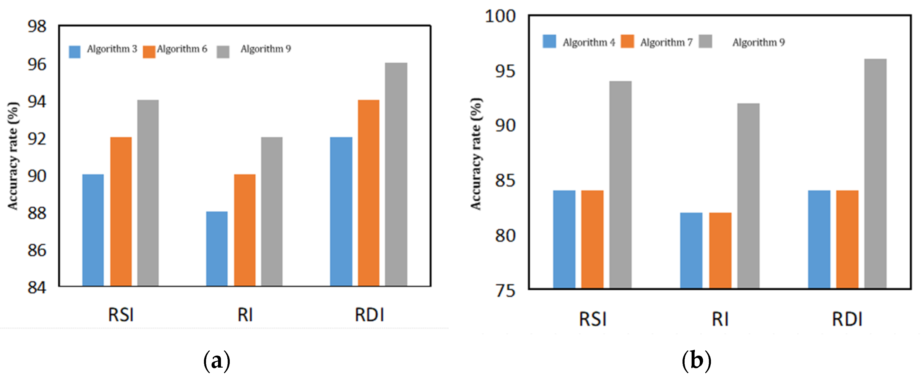
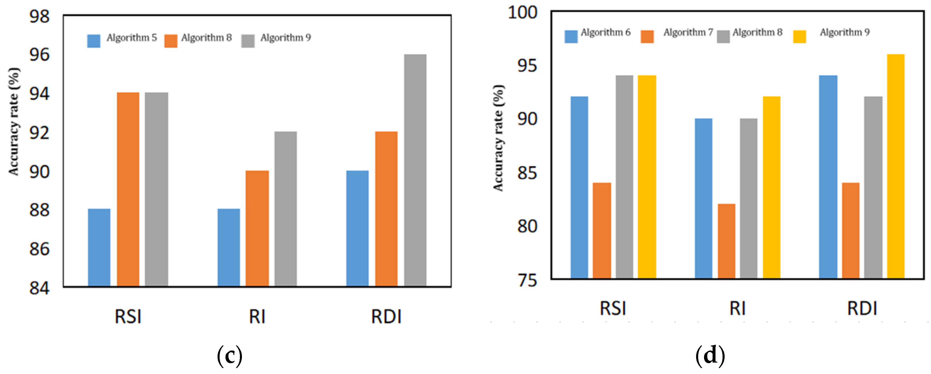
A visual comparison of the forecast accuracy of Algorithms 3–9 leads to Figure 7. As can be seen from Figure 7, the SVM algorithm with adaptive kernel parameter selection shows some improvement over the empirically selected kernel parameter algorithm in forecasting the three indicators of pellet metallurgical performance, which is more prominent in the SVM algorithm with RBF kernel function and Sigmoid kernel function, and no significant change is shown in the SVM algorithm with polynomial kernel function. In addition, Algorithm 9 performs optimally in terms of accuracy in forecasting pellet metallurgical performance indicators, which is superior to the SVM algorithm with a single kernel function, due to the fact that the composite kernel function has both the interpolation capability of the local kernel function and the generalization capability of the global kernel function.
Analysis from the perspective of algorithm running time shows that all of the above nine algorithms are in the acceptable range except for the polynomial kernel parameter adaptive selection SVM method which reaches the maximum number of iterations in the forecasting of RI indicators. In summary, coupling the SVM algorithm of adaptive selection of kernel parameters with the adaptive composite of kernel types is an effective means to improve the forecasting performance of the SVM algorithm, and the target algorithm is obtained based on this design.
The objective algorithm is also an adaptive selection of parameters implemented by means of a genetic algorithm, where the initial parameters (lg(σ), p, q, c, r, ρ1, ρ2, ρ3, log(C)) are set to the optimal kernel parameters and the optimal composite coefficients as described in the previous section. The initial value of the penalty factor C is chosen as log(C0) = −4, and the maximum number of iterations is still chosen as 2000. The relationship between the error and the number of genetic iterations is shown in Figure 7.
The prediction results of the target algorithms for the pellet metallurgical performance indicators shown in the preceding spread and Figure 7 show that the prediction accuracy of the RSI indicator is 100%, the RI indicator is 98%, and the RDI indicator is 100%. Moreover, the number of iterations of the algorithms run is below the threshold of 2000, which shows significant superiority over the nine control algorithms for pellet metallurgical performance prediction applications.
The number of samples selected for this study was 200, and the original ore phases in the samples were relatively easy to obtain. The acquisition of data for the three metallurgical properties of pellets, RSI, RI, and RDI, requires a complex experimental process and large consumables. If the target algorithm designed in this paper can be applied to accurately predict the metallurgical properties of pellet based on the ore phases, the frequency of quality checks in traditional experimental methods can be reduced, further reducing costs.

5. Conclusions

(1) The SVM algorithm was applied to sample data learning and its application effect was found to be limited by the selection of kernel function parameters and the kind of selection, i.e., as long as the appropriate kernel function category and the corresponding class of kernel parameters are used, a good classification performance of the discriminant function can be obtained. Each single kernel function has its own limitations, so the composite kernel function is constructed by combining two or more kernel functions, so the advantages of several other single kernel functions can be taken into account to obtain a superior SVM performance.
(2) In comparison with the nine control algorithms, the target algorithm has the highest forecast accuracy, with 100% accuracy in forecasting RSI grade, 98% accuracy in forecasting RI grade, and 100% accuracy in forecasting RDI grade, and the number of iterations of the algorithm is less than 2000.

Author Contributions

Conceptualization, Y.H. and L.W.; methodology, Y.H.; software, Y.H. and L.W.; validation, Y.H., L.W. and T.X.; formal analysis, Y.H.; investigation, Y.H.; resources, Y.H.; data curation, Y.H.; writing—original draft preparation, Y.H.; writing—review and editing, Y.H.; visualization, Y.H.; supervision, Y.Z., W.W. and T.X.; project administration, Y.H.; funding acquisition, Y.H. All authors have read and agreed to the published version of the manuscript.

Funding

This research was funded by the National Natural Science Foundation of China (NO.52074126).

Institutional Review Board Statement

Not applicable.

Informed Consent Statement

Not applicable.

Data Availability Statement

Not applicable.

Acknowledgments

Thanks to the Hebei Engineering Research Center for the Intelligentization of Iron Ore Optimization and Ironmaking Raw Materials Preparation Processes for training and educating, Thanks to Yang Aimin for his careful guidance. and thanks to classmates in my team for their companionship.

Conflicts of Interest

The authors declare no conflict of interest.

References

  1. Gillespie, G.D.; Everard, C.D.; Mcdonnell, K.P. Prediction of biomass pellet quality indices using near infrared spectroscopy. Energy 2015, 80, 582–588. [Google Scholar] [CrossRef]
  2. Gillespie, G.D.; Everard, C.D.; Fagan, C.C.; McDonnell, K.P. Prediction of quality parameters of biomass pellets from proximate and ultimate analysis. Fuel 2013, 111, 771–777. [Google Scholar] [CrossRef]
  3. Abdollahi, M.R.; Ravindran, V. Influence of pellet length on pellet quality and performance of broiler starters. J. Appl. Poult. Res. 2013, 22, 516–522. [Google Scholar] [CrossRef]
  4. Karamchandani, A.; Yi, H.; Puri, V.M. Fundamental mechanical properties of ground switchgrass for quality assessment of pellets. Powder Technol. 2015, 283, 48–56. [Google Scholar] [CrossRef]
  5. Pomerantsev, A.L.; Rodionova, O.Y.; Melichar, M.; Wigmore, A.J.; Bogomolov, A. In-line prediction of drug release profiles for pH-sensitive coated pellets. Analyst 2011, 136, 4830–4838. [Google Scholar] [CrossRef] [PubMed]
  6. Dwarapudi, S.; Ghosh, T.K.; Shankar, A.; Tathavadkar, V.; Bhattacharjee, D.; Venugopal, R. Effect of pellet basicity and MgO content on the quality and microstructure of hematite pellets. Int. J. Min. Process 2011, 99, 43–53. [Google Scholar] [CrossRef]
  7. Bai, K. Research on Oxidation Roasting and Metallurgical Behaviors of Flux Pellets; University of Science and Technology Beijing: Beijing, China, 2022. [Google Scholar] [CrossRef]
  8. Dwarapudi, S.; Ghosh, T.K.; Shankar, A.; Tathavadkar, V.; Bhattacharjee, D.; Venugopal, R. Effect of pyroxenite flux on the quality and microstructure of hematite pellets. Int. J. Min. Process 2010, 96, 45–53. [Google Scholar] [CrossRef]
  9. Walker, C.T.; Kameyama, T.; Kitajima, S.; Kinoshita, M. Concerning the microstructure changes that occur at the surface of UO2 pellets on irradiation to high burnup. J. Nucl. Mater. 1992, 188, 73–79. [Google Scholar] [CrossRef]
  10. Han, Y.; Lv, Y.; Pan, Y.H.; Zhou, Q.; Yang, A. MComparison of SVM, BP Neural Network and Linear Regression. J. North China Univ. Sci. Technol. 2017, 39, 104–109. [Google Scholar]
  11. Lj, W.; Zy, Z.H.; Yl, L.; Yang, A.-M.; Han, Y. Study on Long and Short-term Memory Networks Model for Intelligent Recognition of Fitness Movements. J. North China Univ. Sci. Technol. (Nat. Sci. Ed.) 2022, 44, 114–120. [Google Scholar]
  12. Yang, A.M.; Han, Y.; Xing, H.W.; Zhang, Y.Z. Building SVM and PNN optimal classifiers based on GA-PLS algorithm and the application in infrared spectrum. Int. J. Adv. Media Commun. 2016, 6, 198–210. [Google Scholar] [CrossRef]
  13. Salimi, A.; Ziaii, M.; Amiri, A.; Zadeh, M.H.; Karimpouli, S.; Moradkhani, M. Using a Feature Subset Selection method and Support Vector Machine to address curse of dimensionality and redundancy in Hyperion hyperspectral data classification. Egypt. J. Remote Sens. Space Sci. 2018, 21, 27–36. [Google Scholar] [CrossRef]
  14. Han, Y.; Li, J.; Li, J.Z.; Xing, H.W.; Yang, A.M.; Pan, Y.H. Demonstration of SVM Classification Based on Improved Gauss Kernel Function. Adv. Intell. Sys. Comput. 2018, 613, 189–195. [Google Scholar]
  15. Yang, A.M.; Han, Y.; Han, C.C.; Xin, Z.C.; Liu, Z.C. Research on Evaluation of Landslide Hazard Based on Ant Colony Algorithm_Support Vector Machine Classifier. J. Comput. Nanosci. 2016, 13, 1117–1123. [Google Scholar] [CrossRef]
  16. Wahab, O.A.; Mourad, A.; Otrok, H.; Bentahar, J. CEAP: SVM-based intelligent detection model for clustered vehicular ad hoc networks. Expert. Syst. Appl. 2015, 50, 40–54. [Google Scholar] [CrossRef]
  17. Kazemian, H.; Yusuf, S.A.; White, K.; Grimaldi, C.M. NN approach and its comparison with NN-SVM to beta-barrel prediction. Expert. Syst. Appl. 2016, 61, 203–214. [Google Scholar] [CrossRef]
  18. Chai, H.Y.; Wee, L.K.; Swee, T.T.; Hussain, S. Gray-Level Co-occurrence Matrix Bone Fracture Detection. Am. J. Appl. Sci. 2011, 8, 26–32. [Google Scholar] [CrossRef] [Green Version]
  19. Vapnik, V.N.; Lerner, A. Pattern Recognition Using Generalized Portrait Method. Autom. Rem. Control 1963, 24, 774–780. [Google Scholar]
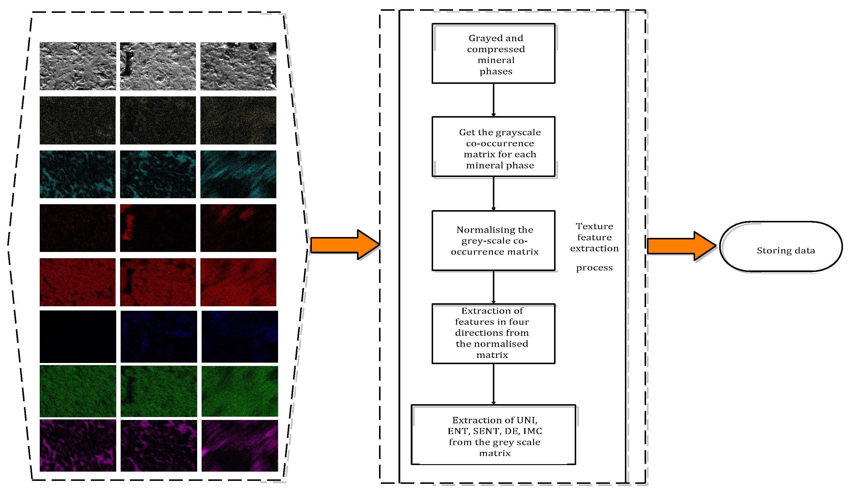
Figure 1. Extraction process of pellet phase texture characteristics.
Metals 12 01662 g001
Figure 2. Initial sample structure for prediction of pellet metallurgical properties.
Metals 12 01662 g002
Figure 3. Schematic diagram of equivalent mapping of kernel function for nonlinear problems.
Metals 12 01662 g003
Figure 4. Chromosome coded bitmap.
Metals 12 01662 g004
Figure 5. Prediction of pellet metallurgical properties based on algorithm 6. (a) The relationship between the number of iterations and the error rate of RSI forecast. (b) The relationship between the number of iterations and the error rate of RI forecast. (c) The relationship between the number of iterations and the error rate of RDI forecast. (d) The best kernel parameter and its corresponding forecast misjudgment rate.
Metals 12 01662 g005aMetals 12 01662 g005b
Figure 6. Algorithm 3, 4, 5, 6, 7, 8, 9 forecast accuracy comparison. (a) Comparison of forecast accuracy of algorithms 3, 6 and 9. (b) Comparison of forecast accuracy of algorithms 4, 7 and 9. (c) Comparison of forecast accuracy of algorithms 5, 8 and 9. (d) Comparison of forecast accuracy of algorithms 6, 7, 8 and 9.
Metals 12 01662 g006aMetals 12 01662 g006b
Figure 7. Prediction of pellet metallurgical performance based on objective algorithm. (a) The relationship between the number of iterations and the error rate of RSI forecast. (b) The relationship between the number of iterations and the error rate of RI forecast. (c) The relationship between the number of iterations and the error rate of RDI forecast.
Metals 12 01662 g007
Table 1. Elite sample set for forecast of metallurgical properties of pellets.
Sample No.Sample InputSample Output
UNIENTSENTDEIMCRSIGrade LabelsRIGrade LabelsRDIGrade Labels
10.5224 0.2592 0.6396 0.6707 0.9955 010002
20.3994 0.4442 0.6485 0.1760 0.1385 001+101
30.3131 0.3336 0.9616 0.0556 0.4454 100002
40.5254 0.0938 0.4998 0.3349 0.3580 010+102
50.0874 0.7117 0.1335 0.4594 0.6743 100−102
60.8858 0.5573 0.1561 0.0601 0.0777 010+101
70.9376 0.4101 0.1480 0.8545 0.5368 010−103
80.3379 0.4173 0.1989 0.7352 0.0657 001001
90.3184 0.3425 0.9681 0.0626 0.4533 100002
100.9974 0.1112 0.1313 0.4972 0.5242 001−102
110.8599 0.5826 0.4807 0.1739 0.8215 100001
120.9418 0.3264 0.0271 0.8841 0.2348 010−102
130.4084 0.4503 0.6501 0.1814 0.1441 001+101
140.4540 0.8743 0.2006 0.8007 0.1423 001003
150.3193 0.3423 0.9631 0.0647 0.4541 100002
160.1222 0.1473 0.7659 0.1289 0.6511 010+103
170.3144 0.3382 0.9701 0.0617 0.4522 100002
180.4506 0.4851 0.8568 0.0991 0.6068 001002
190.9513 0.5520 0.0560 0.4916 0.0511 010−101
200.0187 0.3254 0.6100 0.6238 0.8563 100+102
Table 2. Elite sample set for forecast of metallurgical properties of pellets.
Algorithm Evaluation ParametersMetallurgical Performance IndicatorsAlgorithm 6Algorithm 7 Algorithm 8 Algorithm 9
(n ≦ 2000)RSI2201252731395
RI2752000862412
RDI3221133649405
Q (%)RSI816126
RI1018108
RDI616104
P (%)RSI92848894
RI90829092
RDI94849096
Publisher’s Note: MDPI stays neutral with regard to jurisdictional claims in published maps and institutional affiliations.