1. Introduction and Background
Molecular dynamics (MD) is a powerful tool for understanding the role of microstructure in the deformation and failure response of materials subject to extremely high strain-rate loading. Such fundamental understanding is vital to many applications of national importance [
1,
2] such as armor, space shielding, and stockpile stewardship. Dynamic tensile strength under uniaxial strain, commonly termed spall strength [
3], is particularly sensitive to microstructure and alloy content. These microstructure–spall strength relationships are often non-intuitive and not necessarily simple extrapolations of the quasistatic yield strength-microstructure relationships. For example, pure metals often have higher spall strength than alloys [
4,
5,
6]. The spall strength of single crystals are generally a factor of 2 or 3 higher than the spall strength of coarse-grained polycrystals [
7]. Contradictory to the well-known Hall-Petch relationship, most experimental grain size studies report decreasing spall strength with decreasing grain size [
8,
9,
10,
11,
12]. It has been argued that this anomalous response is due to grain boundaries serving as particularly weak damage nucleation sites [
8,
13]. Generally, higher angle grain boundaries are more susceptible to damage nucleation than low-angle grain boundaries. That said, certain special high-angle grain boundaries, e.g.,
, are more resistant to void nucleation than some low-angle grain boundaries [
11,
14]. The complexity of microstructure–spall strength relationships is further exacerbated in body center cubic (BCC) materials such as Ta, which exhibits two isochoric deformation modes: complex (e.g., non-Schmid effect [
15]) slip systems and twinning [
16].
The fundamental reason why grain boundaries are particularly detrimental to spall strength is not yet fully understood. It is certainly possible that grain boundaries are inherently weaker than grain interiors due to a greater degree of atomic disorder along grain boundaries. Such arguments have been studied in the literature, but no clear correlations between GB energy/volume and spall strength were observed in atomistic calculations of pure Ta [
17]. In alloys, heterogeneous segregation of impurity atoms to grain boundaries may partially explain the apparent weakness of the grain boundaries. Alternatively, or perhaps in combination, local stress concentrations are induced along grain boundaries, which can drive premature failure at the grain boundaries. The stress concentrations are governed by elastic and plastic incompatibilities of lattices on either side of the GB. These effects have been systematically studied via crystal plasticity calculations, finding that elastic and plastic stress concentrations are primarily affected by the tilt component of GB misorientation with the twist component being relatively inconsequential [
11,
18,
19,
20]. MD simulations have also found that both Cu and Ta systems fail more quickly on grain boundaries oriented normal to the load direction due to the higher resolved normal stress [
21,
22,
23]. Strong interactions of dislocations and twins with grain boundaries, e.g., dislocation pile ups and twin-GB intersections, may drive additional stress concentrations along grain boundaries [
21,
24]. Some atomistic studies point to this mechanism being integral to the propensity for intragranular failure in Ta polycrystals due to a high density of intersecting slip systems and twins [
25]. That said, the contribution of each of these mechanisms to GB spall failure is not yet fully understood in pure or alloyed materials.
Normal plate impact tests are the most common configuration to experimentally probe the spall behavior of materials [
26].
Figure 1, reproduced from Chen et al., shows a diagram of their flyer-plate simulations for reference [
21]. Such tests consist of a flyer plate being launched at high velocity into a target plate initially at rest. The impact generates compressive shock waves that propagate through the thickness of the flyer and target plates, shown in red dotted lines. These waves progress diagonally to show them moving with time. A compressive wave (red) passes the GB before rarefaction at the free surface, and later the rarefaction waves (blue) meet at the GB. By construction, the deformation is one-dimensional with a macroscopically uniaxial strain state induced.
In this type of simulation, the aspect ratios, plate diameters normalized by plate thicknesses, of both plates are typically greater than 5 to minimize contamination of the one-dimensional uniaxial state by release waves emanating from the lateral surfaces. This compressive shock typically induces plastic deformation and a temperature rise, both of which can alter the material microstructure, e.g., dislocation density. Since spall strength is sensitive to such shock-induced microstructural changes, spall strength unfortunately becomes a poorly defined material property that is sensitive to the test conditions, e.g., shock pressures, shock durations, shock rise times, and shock profiles. Often, simulations adopt a similar test configuration by making use of flyer and target “plates” that are tens or hundreds of nanometers in thickness. While this results in MD simulations that more closely mimic the nature of the plate impact experiments, albeit with short length and time scales [
27], it also preserves the unfortunately complex dependence on test conditions that cloud the interpretation of spall strength as a material property.
To overcome this shortcoming of plate impact MD simulations, here we advocate the use of shock-free homogeneous deformation of MD samples. The homogeneous simulations have two major advantages. Firstly, these simulations enable the de-coupling of spall strength and shock-induced microstructural changes that depend on shock pressures, shock durations, shock rise times, and shock profiles. This enables a more systematic understanding of the role of microstructure on the fundamental dynamic tensile strength of a material with known microstructure. Secondly, these simulations often require roughly two to three orders of magnitude fewer atoms and similarly lower computational costs than comparable plate impact MD simulations. The large system sizes required for plate impact MD simulations are typically driven by the longitudinal lengths required to form a quasi-steady shock profile. In addition, relatively long simulations times are required for the shockwaves to propagate to the free surface of the target plate and reflections to subsequently arrive at the spall plane. On the other hand, the system size for homogeneous MD calculations is driven entirely by the microstructure with the smallest possible representative volume element that captures all relevant microstructural features being the lower bound on system size. For many materials of interests, e.g., single crystals or bicrystals of pure or solution strengthened alloys, this lower bound is quite small. It is also reasonably small for some nanocrystalline materials [
28,
29]. Here, we will directly compare our 24,000 and 200,000 atom homogeneous MD calculations with 20 million atom plate impact simulations of BCC Ta published by Chen et al. [
21]. Both simulation methods result in similar non-monotonic dependencies of GB misorientation on spall strength. That said, the homogeneous MD calculations are significantly less computational expensive by a factor of
for 24,000 atoms and
for 200,000. However, the accuracy of the results seems to be reduced somewhat from the smaller simulation size, relative to the shock simulation results. The datasets are compared in
Table 1.
The structure of the paper is as follows.
Section 2 describes the computational methodology used here.
Section 3 presents the results and discusses the comparison between these results and those from Chen et al. [
21]. Finally, a summary is given in
Section 4.
2. Methods
Here, we simulate the spall failure of bicrystal BCC Ta containing a single tilt GB aligned normal to the impacting projectile. Similar configurations have been adopted previously in crystal plasticity simulations, e.g., Nguyen et al. [
18,
19], as well as in experiments on bicrystals and tri-crystals target plates, c.f. [
30]. Our simulations show the behavior of a single GB explicitly, without resolving the entire polycrystalline structure common in spall experiments. Additionally, the GBs are modeled as perfectly bonded interfaces, without the effect of local GB characteristics. All GBs in this work have a loading direction parallel to the GB normal, which is most susceptible to failure [
10,
31,
32]—up to an order of magnitude more likely to nucleate a void than loading directions perpendicular to the GB normal [
17]. The orientation allows the probing of properties versus misorientation angle without needing to factor in the effects of the GB’s orientation with respect to the loading direction, which was found to be sometimes significant [
17,
20]. A large benefit of this method is allowing for reduced simulation size and computational time.
We construct and study bicrystal BCC Ta specimens with a single symmetric tilt GB in the middle of the specimen as shown in
Figure 2. The GBs studied here are all coincident site lattice (CSL) boundaries. The GBs are generated using the MD simulator LAMMPS (Large-scale Atomistic/Molecular Massively Parallel Simulator), specifically by joining the two crystals at the GB plane and deleting any overlapping atoms [
33]. Grain boundaries are visualized in OVITO. Two atoms are defined to be overlapping if they are within a specified cutoff radius of each other. In initial runs, this radius was varied from 0 to 2.1 Å to test its significance (for reference, Ta’s atomic radius is 2.2 Å). Cutoff radii that are too small leave atoms partially inside of one another, which generates a very high initial compressive stress state that perpetuates throughout the simulation, giving unrealistic results. Once the cutoff radius is large enough to remove the overlapping atoms at the GB, further increases make no difference until the atomic separation distance in the lattice is reached, at which point every atom would be deleted. The cutoff radius used here (1.64 Å) is large enough to avoid artificial initial compressive stress states while remaining below the atomic separation distance. This procedure to generate GBs is consistent with the methodology adopted in Chen et al. [
21].
Simulations for the set of boundaries were run at two box sizes to investigate the simulation size effects. For the smaller set, the simulation box size is chosen to be 20 repeated unit cells in the
and
directions, with 30 unit cells in the
direction which is the direction of deformation. That makes the total size
in
and
, and
in
, with
atoms (not exact because of edge effects and removing overlapping atoms) and periodic boundary conditions in all three dimensions. The other set of simulations was run doubling the size along each dimension, with
atoms. These simulation domain sizes are substantially smaller than the size adopted by Chen et al. with its 15–20 million atoms [
21]. The interatomic potential used here is the Ta2 EAM (embedded atom model) potential by Ravelo et al. [
34]. This is the same potential used by Chen et al., and agrees well with model generalized pseudopotential theory calculations performed by Moriarty et al. for pure Ta systems up to ~180 GPa [
21,
34,
35].
Throughout deformation, a system level stress tensor is computed via a summation of the kinetic energy tensor and the virial tensor, i.e.,
Here, is the number of atoms, is the system volume, and is the mass of the -th atom. The position, velocity, and force vectors associate with the -th atom are, respectively denoted as and . Throughout this work the component of the component of the stress tensor, i.e., will be reported and analyzed. This component of the stress tensor represents the axial normal stress aligned with the direction of uniaxial deformation.
The simulation for each GB proceeds through three stages: (1) an initial minimization stage that relaxes the atoms to minimum energy positions, (2) a compressive stage that replicates the passage of a compressive wave before spall and generates defects in the otherwise perfect lattice, and (3) a tension stage that deforms the material until failure to measure its strength. The last two stages approximate the loading conditions generated by the passage of a compressive shock wave and subsequent tensile (spall) failure induced by release wave interactions, following the similar procedures advocated by Nguyen et al. [
18,
19].
In the minimization stage, the unrelaxed GB formed by joining two crystals in LAMMPS is relaxed by giving each atom a random initial velocity corresponding to temperature, 300 K. Then, the simulation progresses at 300 K for 50 picoseconds (ps) using the NPT ensemble (holding number (N) of particles, system pressure (P) and temperature (T) constant) to relax atoms to equilibrium positions. Three seeds were used to generate initial velocities to test stochasticity. The mean spall strength from the three seeds is reported for each misorientation angle.
After minimization, the GB is compressed in the direction to uniaxial engineering strain over 25 ps to approximate the passage of a GPa compressive shock wave, which nucleates somewhat realistic crystallographic defects (e.g., dislocations) in the grains. The compressive stage is carried out at a strain rate of while relaxing with the NVE ensemble (holding number (N) of particles, volume (V) and energy (E) constant) at each timestep.
The final stage of the simulation is the tensile portion, wherein the GB is pulled along the -axis until failure using the same strain rate as in the compressive stage. This replicates the tensile stresses experienced at the GB from rarefaction waves interacting in spall. The point of maximum stress in this stage is indicative of the first void nucleation since the material will resolve the stress through deformation. Thus, we use ultimate tensile stress (under uniaxial strain conditions) as a proxy for cavitation strength. Data from the simulation are output every picosecond. This limits the accuracy of the method relative to the rate of tensile stress change, since a void could nucleate between outputs. The accuracy of the spall strength measurements in this work are thus .
3. Results
Analyzing how the stages of the simulations progress on a representative GB gives insight about what exactly is happening in the simulations. From the
GBs explored in this work, the GB that was selected for this illustration is the
° misorientation angle GB with
atoms shown in
Figure 2 and
Figure 3.
The effects of the minimization stage can be seen by contrasting
Figure 2a with
Figure 2b and
Figure 3a with
Figure 3b. Before minimization, there are pockets of empty space between the grains, seen in white in
Figure 2a and
Figure 3a. The coloring in
Figure 3 denotes the centrosymmetry parameter, which measures the degree of local lattice disorder, representing defects surrounding each atom. The blue regions are the closest to a perfect lattice, and the red regions have the highest lattice disorder, representing defects. Centrosymmetry is calculated using the following equation, with 8 nearest neighbors (
) for BCC [
33].
Figure 2e and
Figure 3e show the system after the compressive stage has completed and was additionally pulled in the tensile stage until the system returned to its initial size as
Figure 2b and
Figure 3b. Contrasting this with
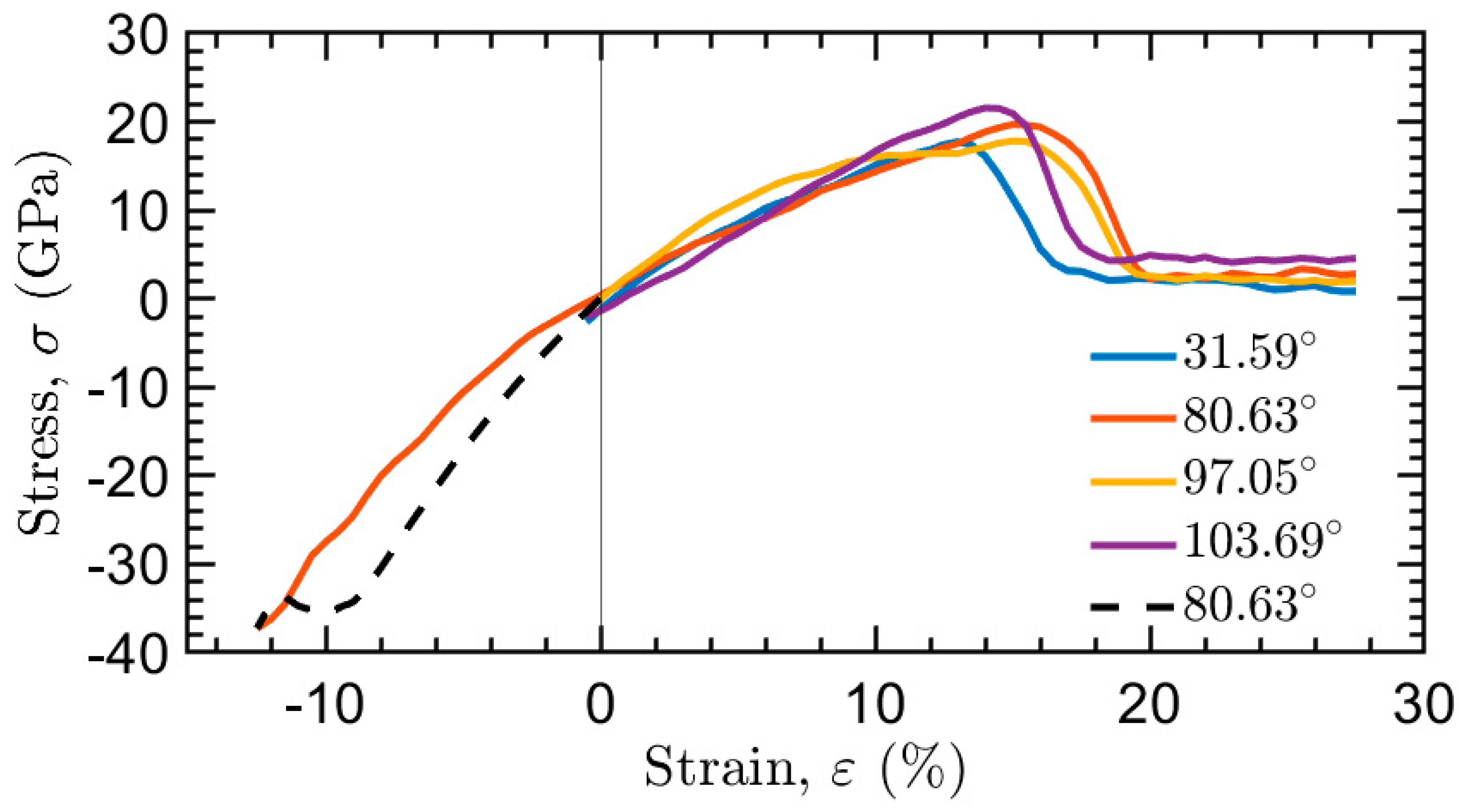
Figure 3b, colored regions of defects generated from the deformation are visible that were not present previously in the system. This shows the defects generated by the compressive stage, and why it is implemented in the simulations. Because of this, these are plastic deformations that change the structure for the tensile stage, which is the goal of the compressive stage. This can be seen in the hysteresis between the compressive and tensile curves in the stress–strain diagram presented in
Figure 4, showing the energy lost to plastic deformation. Additionally, notable on the stress–strain diagram in
Figure 4 is a local minimum in tensile stress at about
tensile strain. The minimum in the curve represents the defect nucleation point.
The tensile portion of the simulation generates larger and larger tensile stresses until failure, shown in
Figure 4. This deformation grows the defects generated by the compressive stage, with the colored portions in the bottom left and top right of
Figure 3e turning into the dislocations seen in
Figure 3g. There is also more lattice disorder at the GBs in
Figure 3g, both in the center and the top and bottom due to periodic boundary conditions. Eventually, this leads to the material failure shown in
Figure 3h.
These steps were repeated for all
GB misorientation angles examined by Chen et al. [
21]. The main advantage in the method used in this work is achieving a speedup in computational time for simulations. The simulations run in the present work used about
and
atoms for 155 ps. Run on only one core, each smaller simulation took 30 min, and the larger size simulations took 3–4 h. Chen et al. used simulations with 15–20 million atoms for a total of 110 ps [
21]. Run on 180 cores, they took 2.5 h per trial. The computational time decreases linearly with the number of cores up to 2000, so the speedup in this paper is on the order of
and
for the two sets when compared on the same number of cores. The present work aims to validate this model against the results from Chen et al. [
21] by testing cavitation strength vs. GB misorientation angle on the same GBs.
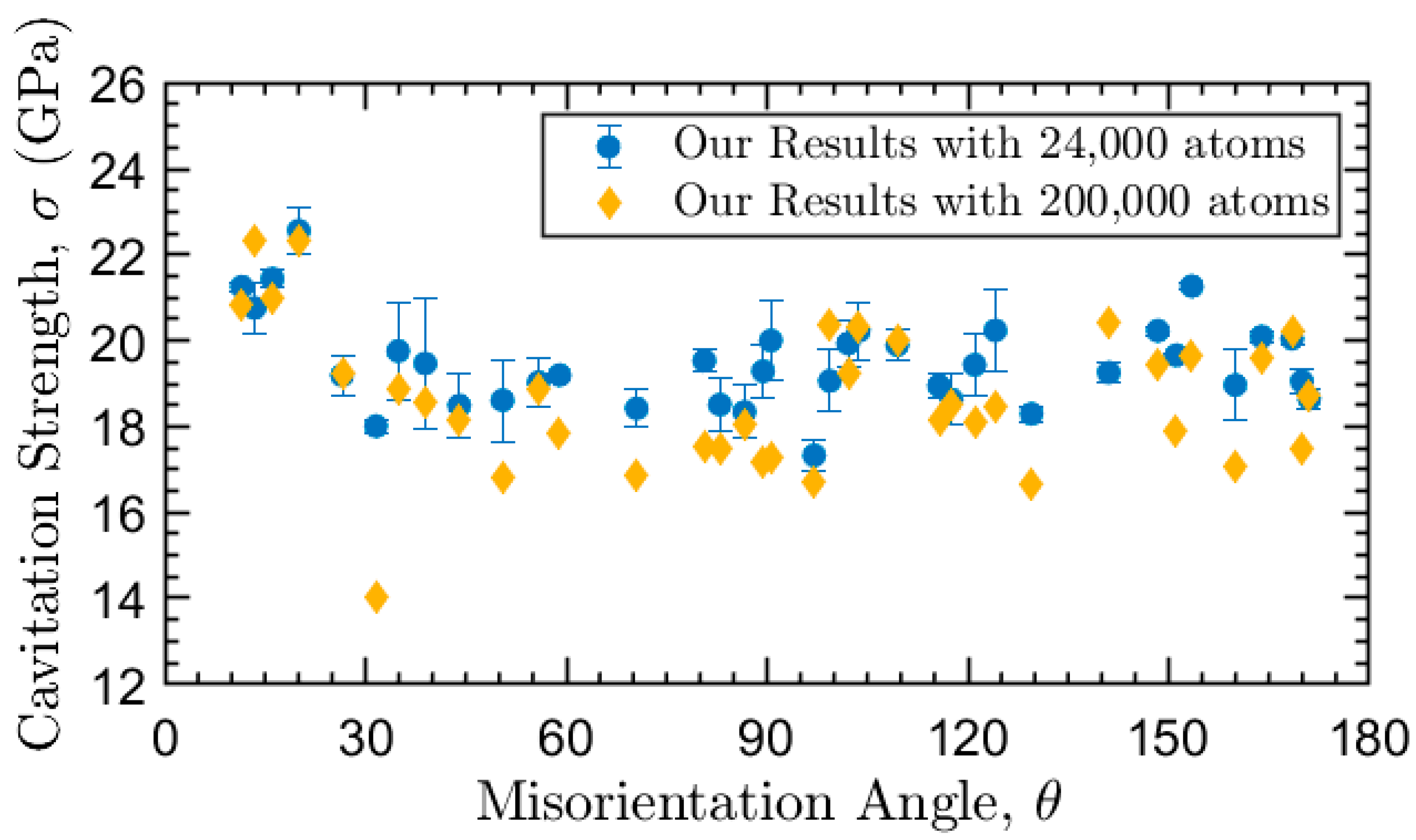
Figure 5 shows the void nucleation stress vs. GB misorientation angle for the simulations carried out in this work and Chen et al., both with the same GBs [
21]. Our results show similar predictions for void nucleation stress through the misorientation space studied here, apart from a vertical shift in the data. Additionally, notable is a much better agreement between the two datasets in the 0°–125° region, with worse agreement at high angles, 125°–180°. We are not certain of the reason behind this, but a possibility is that at high angles, there is more free volume at the GBs, and thus a more stochastic nature at the sizes studied. The vertical shift in the results from our smaller dataset averaged 2.29 GPa higher than those of Chen et al., a difference of about 10%, and the results from our larger dataset averaged 1.25 GPa higher than the data of Chen et al., a difference of about 5% [
21]. Two possible factors influencing this vertical shift were investigated and are discussed shortly. Additionally, the dispersion of the data points in this work is greater than that of the data from Chen et al. [
21]. This is likely because they varied local structure for each GB, averaging two local structures per GB to obtain each data point. Our results came from a single set of local properties per GB, which intrinsically has more variance. In future work, we hope to leverage the faster simulation time of this method to test spall strength response to local GB properties.
The first possible explanation for the vertical shift in void nucleation stress is size effects, because the two sets of simulations from this work were run with two and three orders of magnitude fewer atoms than those of Chen et al. [
21]. Finding the effects of simulation size was the primary motivation of running simulations for all 37 GBs at two different sizes. Our results with 24,000 atoms and 200,000 atoms are compared in
Figure 6. The larger dataset agreed more closely with results from the flyer/plate experiments performed by Chen et al., with a mean difference of 1.25 GPa compared to 2.29 GPa from our smaller dataset [
21]. The trends with misorientation angle remained similar for both size datasets. To further study the effects of the simulation size, the size of a single system is varied in orders of magnitude by doubling the size in all three dimensions, which increases the number of atoms by a factor of 8. The results are shown in
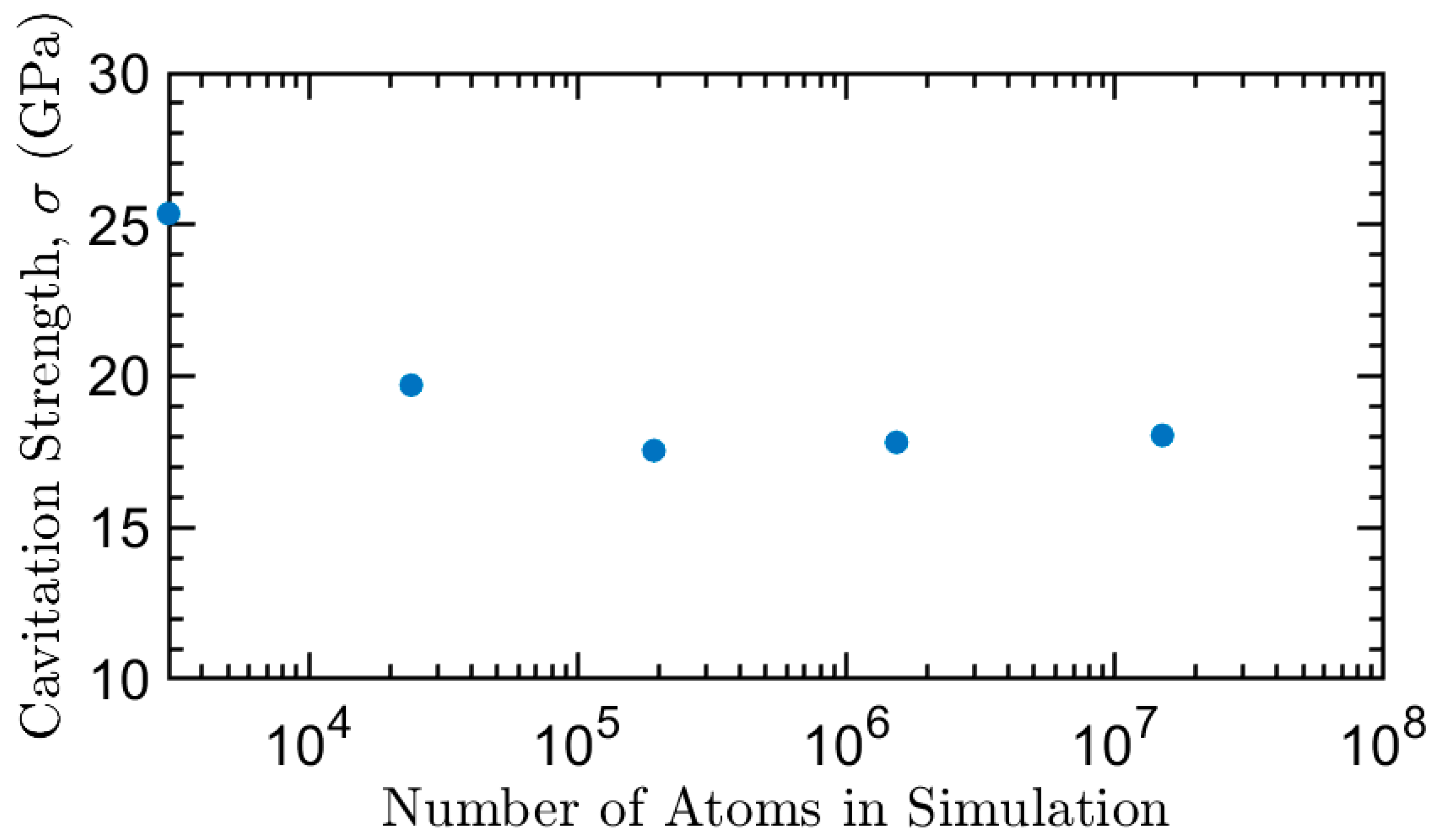
Figure 7, which contains more sizes than were studied for all 37 GBs.
Figure 7 shows the void nucleation strength versus number of atoms in the simulation for a BCC Ta bicrystal with misorientation angle of 80.63°. The second data point from the left shows our result for this boundary with 24,000 atoms, and the third data point shows our result with 200,000. The fifth data point is the result from Chen et al. for the same GB [
21]. The data point on the far left shows that running our simulation with even fewer atoms (3000) increases the gap relative to the result from Chen et al. [
21]. Conversely, as the size of the simulations increase, the third and fourth data point trend towards the result from Chen et al. [
21]. The mean difference between the void nucleation stress data presented here with
atoms and those of Chen et al. [
21] was 2.29 GPa, whereas the mean difference with
atoms was 1.25 GPa, so this could explain why there is a vertical shift in our data. This suggests that our results might agree quite closely if the simulations were performed on the same length scale.
Another size effect that was noted is that smaller system size increases the dependence on initial conditions. Changing the seed in LAMMPS that determines initial random atomic velocities introduces some stochasticity to smaller simulations. Void nucleation stress results for the 24,000 atom dataset varied by up to 20% with changing seed for one misorientation angle, though most differed by less than 5%. However, the average void nucleation stress across the runs does not change, nor does the trend of dependence with misorientation angle. To account for this, we report the mean spall strength for each misorientation angle using three random seeds, and included standard error bars on
Figure 5 and
Figure 6, the figures that report on the 24,000 atom dataset.
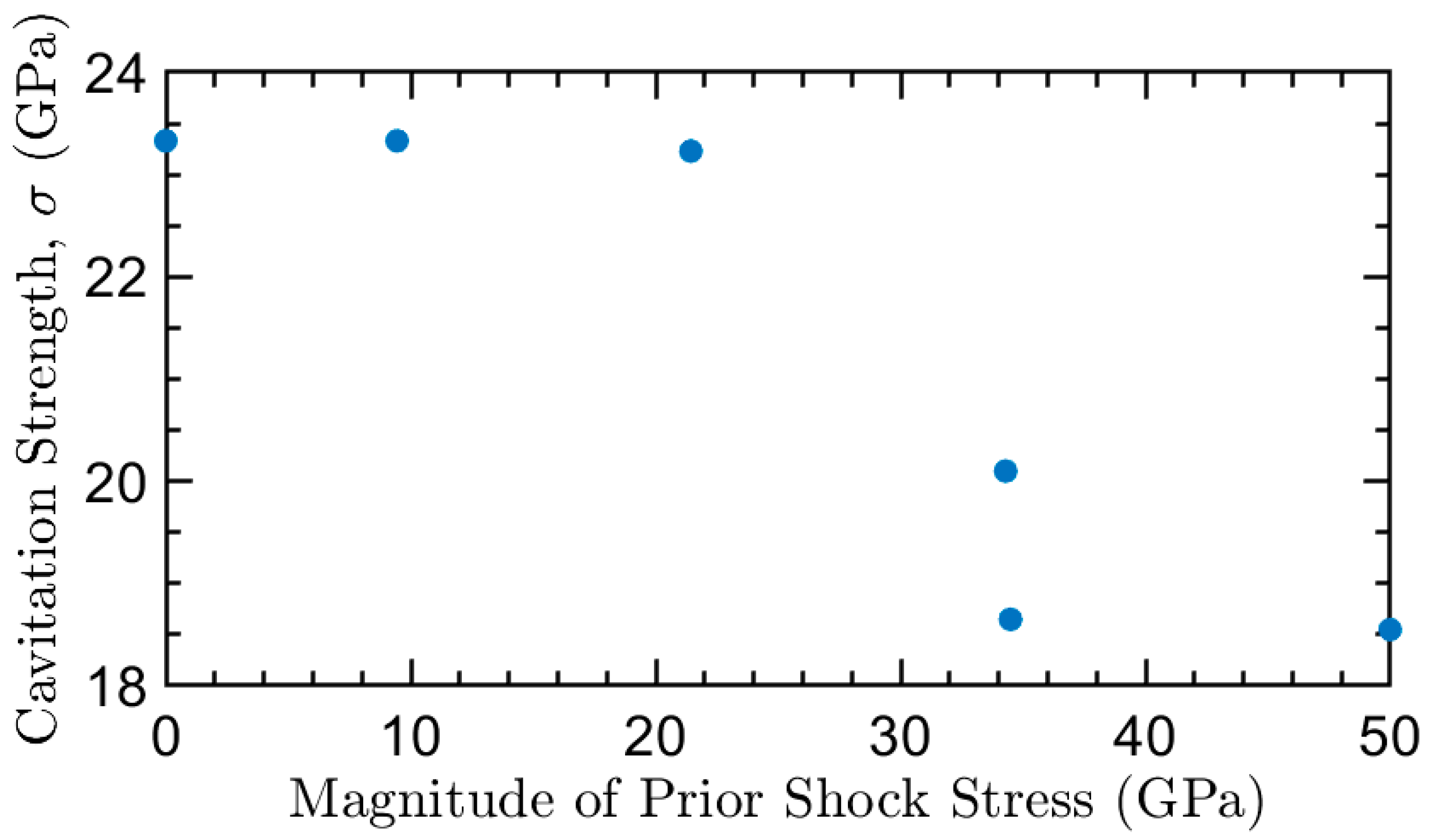
To investigate another possible reason for the vertical shift in void nucleation stress, the degree of compression during the second stage of the simulation was varied from 0 to 50 GPa in
Figure 8, with linearly increasing compressive strain for each point. Because each point is set at a fixed strain level, the stress levels are not evenly spaced. At 0 GPa of compressive stress, the tensile portion of the simulation is trying to deform a perfect crystal, which is harder to do than when defects are present. This is because deformation often happens through the motion of dislocations, which requires dislocations to be formed and to be moved. The stress to form new dislocations is higher than the stress required to move them, so lattice that already contains defects will have lower strength. The 0–20 GPa runs (the first three data points) did not have enough stress to nucleate defects in the material, so they all had similar cavitation strengths.
The most interesting results come from the fourth and fifth datapoints, around 35 GPa in compressive stress. The slightly higher point has 25% less compressive strain, but almost the same stress. That is because the compressive stress is partially resolved in the material through deformation. Thus, we can see that defects are generated at around 35 GPa. After that point, the cavitation stress does not decrease further when compression is increased to 50 GPa, reinforcing the importance of the 35 GPa range. This does not describe the difference between the results, but it does give some insight about what is happening in the compressive stage.


