1. Introduction
The structural integrity of the dissimilar metal weld (DMW) joints connecting the ferritic steel pipe nozzles of the pressurized water reactor vessels with the austenitic stainless steel safe-end is critical to the safe operation of nuclear power plants. The safe-end is a pipe segment measuring about 200 mm long usually made from austenitic stainless steel (typically 316L). One end is connected to the nozzle of the reactor pressure vessel using the specifically designed DMW joint, and the other end is connected to the primary coolant loop pipe (made of stainless steel) using a similar metal weld joint. The pressure vessel, safe-end and primary piping are therefore joined together to form the primary pressure boundary of the nuclear power plant. The DMW is made in the workshop, after the inner wall of the nozzle is cladded and buttering layers added, which is then followed by a stress relief heat treatment procedure. Similar metal welding is then carried out onsite. Both the DMW and the onsite similar metal weld are not post-weld heat treated, in order to avoid the possible sensitization effects. As these welded joints are put into service in the as-welded conditions, it is reasonable to believe that they would contain high levels of tensile residual stress, which is considered to be detrimental.
It is also known that these DMWs are prone to stress corrosion cracking (SCC) in service operational conditions, and welding residual stresses have been recognised as one of the important factors that promote SCC [
1,
2]. In addition, both the manufacturing induced residual stress and in-service thermal stress could affect the susceptibility to hydrogen embrittlement (HE) of the material, which is closely related to the in-service brittle fracture of a structural component of a nuclear power plant [
3]. It is therefore of paramount importance to understand the level and distribution of these residual stresses, as well as their formation and evolution mechanisms, in order to quantify their detrimental effects and ultimately bring them under control in the long run. For this reason, considerable research effort has been devoted into this area so far [
4,
5,
6,
7,
8,
9,
10,
11,
12].
For example, Coules et al. [
4] studied the residual stresses in a Control Rod Drive Mechanism (CRDM) nozzle attachment weld of a Pressurised Water Reactor (PWR) using a deep hole drilling method. They discovered that although modest tensile stresses occurred in the cladding, the attachment weld contained tensile residual stresses of yield magnitude. Guo et al. [
5] investigated the laws of stress and strain distribution at the SCC crack tip under the interactive effect of residual stress and mechanical heterogeneity in a nuclear power plant safe-end by means of theoretical analysis and finite element method. Their research results showed that due to the variation of the residual stress, the propagation of the SCC crack might even be paused. Tan et al. [
6] investigated the effect of welding residual stress on operating stress in designing a nuclear turbine welded rotor. They employed a 2D axisymmetric finite element model in their study and showed that the operating stress can be affected significantly by the welding residual stress, and the distribution trend of the superposition stress in the weld area was mainly determined by the welding residual stress.
Liu and Wang [
7] performed finite element analyses to study the effect of weld overlay sizing on residual stresses of the DMW in PWRs in order to provide a reference for optimizing the weld overlay design. Koo et al. Ref. [
8] used cascaded support vector regression (CSVR) to estimate the residual stresses in welded dissimilar metals at nuclear power plants. Song and his partners [
9,
10] proposed approximate expressions for calculation of through-wall welding residual stress distributions in DMWs of PWR nozzles. In the expressions that they put forward, it was assumed that welding residual stresses were dependent upon the wall thickness of the nozzle, the radius-to-thickness ratio and the 1.0% proof strengths of the base and weld metals, but not on the safe-end length. Wen et al. [
11] conducted a stress analysis for the coolant pump nozzle of a nuclear reactor pressure vessel and found that the ANSYS/WORKBENCH approach was more convenient than the traditional ANSYS APDL method in the geometry modelling, loading and post processing. Liu [
12] clarified the effects of a material hardening model and lumped-pass method on a welding residual stress simulation of a J-groove weld in a nuclear RPV (reactor pressure vessel). It was found that based on the kinematic hardening model, the residual stresses simulated with the lumped-pass FE model were almost consistent with those obtained by the pass-by-pass FE model.
Due to the complex nature of the residual stresses in the DMWs, the finite element (FE) modelling technique has been employed in most investigations carried out and reported in the literature. For instance, Dehaghi et al. [
13] investigated the residual stresses in feed water nozzle joints in the primary circuit of nuclear power plant reactors using the commercial FE software package ABAQUS. It was discovered that the difference in thermal expansion coefficients between the stainless steel material of the safe-end and the weld metal had led to the creation of tensile residual stresses in the stainless steel zone with high magnitudes. Lee et al. [
14] conducted three-dimensional thermal elastic–plastic FE analysis that accurately predicted the residual stress states in the DMWs joining carbon and stainless steel pipes. They found that the axial and hoop residual stresses in the base metal near the weld region on the stainless steel pipe side were higher than those on the carbon steel pipe side in both the inner and outer surfaces. The EPRI/NRC WRS program organized by the Electric Power Research Institute (EPRI) and the U.S. Nuclear Regulatory Commission (NRC) included a round-robin modelling activity on biaxial weld residual stress (WRS) mapping for a DMWed nozzle, where a number of research teams submitted their weld modelling results blind to the experimental measurement data [
15]. It was found that despite the large spread in the modelling outputs, there was still a level of agreement between the measurement data and model average, both in terms of hoop and axial residual stresses. In this work, the contour method was used to measure the hoop residual stress and the slitting measurement was used to determine the axial residual stress [
15]. A few researchers also employed hole-drilling method [
1,
4,
16] and neutron diffraction technique [
17,
18] to characterise weld residual stresses and validate the modelling results.
On the other hand, attempts were also made to introduce compressive residual stresses in order to suppress crack propagation in the originally deposited weld metal. In trying to do so, Chu et al. [
19] used an overlay weld of 10 mm thick on top of the original stainless-steel T-pipe joint. The contour method was employed to measure the residual stress in the T-joint and it was shown that compressive residual stress of about 50 Mpa was formed in the original ER316L weld. Ahonen et al. [
20] showed in their work that by thermal ageing at 400 °C, the strength mismatch at the SA 508/Alloy 52 of a narrow-gap dissimilar weld could be markedly reduced, which is believed that the effect of strength mismatch reduction at the interface may also help reduce the tensile residual stresses in the weld joint.
From the brief literature review conducted to date, it is highlighted that high level tensile residual stresses of yield magnitude are expected in the nuclear safe-end DMW joints and that the detailed distribution, in particular the through-wall variation, is of significant interest for their safety and structural integrity assessment. Although the various numerical and analytical techniques can provide such data, their validation using equivalent experimental results have been scarce. Like XRD, the hole-drilling technique can only provide surface or near surface measurement. On the other hand, the deep-hole-drilling method could be used to measure through-thickness variation of residual stresses, however the measurement results are subject to the selection of measurement location and the accuracy is also sometimes questionable due to low spatial resolution (averaging over the hole diameter). It is well known that both neutron diffraction and the contour method can be used to perform through-thickness residual stress measurements with high spatial resolution as well as accuracy. Nevertheless, up to now there have been few reports on the characterisation of residual stresses of DMWed structures with particular relevance to nuclear applications by using these techniques. It is thus recognised that there is a strong demand for a better understanding of the detailed residual stress distributions in the nuclear safe-end DMW joints through further development of numerical modelling techniques that are validated by experimental data obtained using reliable and thorough experimental characterisation methods, in order to enrich the portfolio of high-fidelity residual stress data.
In this study, a mock-up of a nuclear safe-end DMW joint (SA508-3/316L) is manufactured, and the weld residual stresses are thoroughly characterised using neutron diffraction and the contour method. A detailed finite element modelling exercise is also carried out for the prediction of the weld residual stresses resulting from the manufacturing processes of the DMW joint. Finally, for model validation purposes, the FE modelling results are compared with those of the experiments, and good agreement has been attained.
6. Conclusions
In the current study, a mock-up of a nuclear safe-end DMW joint (SA508-3/316L) was manufactured, by closely following the standard procedures for nuclear applications. The weld residual stresses of the mock-up in its final machined condition were thoroughly characterised using neutron diffraction and the contour method. Alongside with the experimental work, a detailed finite element modelling exercise was also carried out for the prediction of the weld residual stresses resulting from the manufacturing processes (mainly the multi-pass girth welding and the final machining) of the DMW joint. From the analysis and comparison of the residual stress results between the FE prediction and experimental measurements, the following conclusions can be drawn:
(1) After multi-pass girth welding, high level tensile residual stresses are predicted by the FE simulation, mostly in the weld crown and weld toe areas on the OD and the sharp corner near the weld root on the ID of the DMW joint, with the maximum values well above 500 MPa in the radial, axial and hoop directions. Although these values are significantly higher than the calculated initial yield stress of the filler metal due to strain hardening in the FE calculation and may represent an artifact, it is still recommended that precautions should be taken when these welded structures are put into service, preferably after the weld joints are treated for stress relief.
(2) After mechanical machining, the materials containing high value residual stresses including those geometrical stress concentrators have been removed and the residual stress field has reached a new equilibrium condition. Therefore, the maximum values of the various residual stresses are drastically reduced by up to 76.6% (in the radial direction), suggesting that having the weld crown and root machined off by cutting or grinding would be a good practice in reducing the detrimental high level tensile residual stresses in the welds.
(3) In the final machined condition, the FE results show low level of tensile residual stresses in the ID area of the weld seam and compressive residual stresses in the ID of the adjacent SA508-3 and 316L material, which would be beneficial in inhibiting the development of SCC. According to the FE calculation, high level tensile residual stresses are found predominantly in the hoop direction in and near the multi-pass girth weld joint, tending towards the OD with a maximum value of about 467.7 MPa. In the axial direction, relatively high tensile residual stresses are found near the OD surface of the weld joint, extending into the SA508-3 side with a maximum value of about 242.2 MPa (about half of that in the hoop direction). In the radial direction, moderately high tensile residual stresses are found along the weld (INCONEL52M) and 316L fusion boundary with a maximum value of about 134.8 MPa (about half of that in the axial direction). While not in direct contact with corrosive medium, the high level of tensile residual stresses in the OD of the DMW joint may favour fatigue crack initiation and growth.
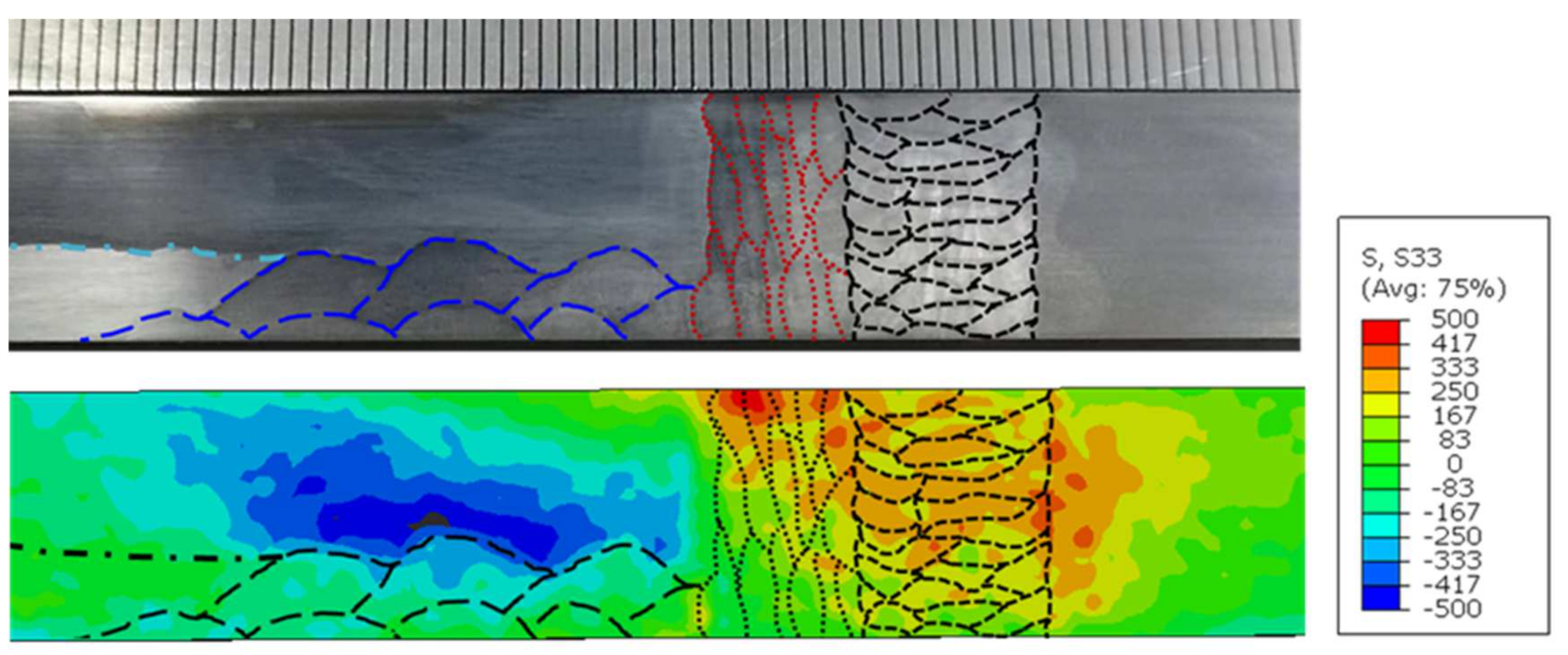
(4) The hoop residual stress distribution near the DMW joint of the mock-up as derived from the contour method bears close resemblance to that from the FE prediction. The maximum tensile hoop residual stress determined using the contour method was about 500 MPa, which compares very well with the FE predicted value of about 467.7 MPa. Along the neutron scan line at the OD subsurface across the weld joint, both the contour method and the FE modelling gave maximum hoop residual stress near the weld fusion line on the 316L side at 388.2 MPa and 453.2 MPa respectively, whereas the neutron diffraction measured a similar value of 480.6 MPa in the buttering zone near the SA508-3 side. Therefore, it is demonstrated that the contour method is also effective in quantifying residual stresses through the entire cut-plane, despite its drawbacks of being a destructive method.
(5) Detailed comparison of the hoop residual stresses along three paths across the girth weld joint near the OD, mid-wall and ID has revealed that residual stresses obtained using the three different methods, namely the neutron diffraction technique, the contour method and the FE modelling analysis, are reasonably consistent. In particular, the agreement between the hoop residual stress distribution patterns in the girth weld and the 316L material obtained from the three techniques is excellent for all the three paths evaluated, although slightly higher values are recorded by the neutron diffraction measurement along the mid-wall and ID. Therefore, it has been demonstrated that the methodology and techniques adopted in the current investigation of the residual stresses in the DMW joint of a nuclear safe-end mock-up are valid and effective. The minor discrepancies between the FE prediction and experimental measurement of the hoop residual stresses found in the buttering and SA508-3 areas are primarily due to the inadequate assumptions made in the FE modelling, i.e., by ignoring the inherent effect of the cladding and buttering residual stresses that may not have been completely removed by the stress relief heat treatment applied in practice. These conclusions are worthy of further investigation.
Author Contributions
Conceptualisation, methodology and supervision, S.Z.; writing—original draft preparation, Z.F., J.L. and S.W.; writing—revised draft, review and editing, S.Z., S.W., S.P., Z.F. and J.L.; FE modelling and formal analysis, Z.F. and J.L.; experiments, data analysis and comparison, S.P.; funding acquisition, S.Z. and L.L.; investigation, S.L. and L.L. All authors have read and agreed to the published version of the manuscript.
Funding
The work reported in this paper was financially supported by the Guangdong Major Project of Fundamental and Applied Fundamental Research (Project No. 2019B030302011 and 2020B0301030001), the Stable Supporting Fund of Science and Technology on Reactor Fuel and Materials Laboratory (Project No. JCKYS2019201073), the Guangdong Innovative and Entrepreneurial Research Team Program (Project No. 2016ZT06G025), and the Guangdong Natural Science Foundation (Project No. 2017B030306014).
Institutional Review Board Statement
Not applicable.
Informed Consent Statement
Not applicable.
Data Availability Statement
Not applicable.
Acknowledgments
Sincere thanks are given to Zhifeng Gong, Neutron Technology Department, Centre of Excellence for Advanced Materials, Dongguan, Guangdong Province, China, who participated in the neutron experiment and collated the raw data; to Tung Lik Lee and Saurabh Kabra, ISIS Facility, Rutherford Appleton Laboratory, Didcot, UK, who facilitated and supported the neutron experiment at ENGIN-X; and to Stephen Nneji, also from ISIS, who provided SScanSS-2 software support ISIS Facility, Rutherford Appleton Laboratory, CCLRC, Chilton, Didcot, OX11 0QX, UK. The ENGIN-X beamtime awarded through their Rapid Access Application (RB2000033) is also gratefully acknowledged.
Conflicts of Interest
The authors declare no conflict of interest.
References
- Lee, K.S.; Kim, W.; Lee, J.G. Assessment of possibility of primary water stress corrosion cracking occurrence based on residual stress analysis in pressurizer safety nozzle of nuclear power plant. Nucl. Eng. Technol. 2012, 44, 343–354. [Google Scholar] [CrossRef]
- Jenssen, A.; Norrgard, K.; Iagerstrom, J.; Embring, G.; Tice, D. Assessment of cracking in dissimilar metal welds. In Proceedings of the 10th International Symposium on Environmental Degradation of Materials in Nuclear Power Systems—Water Reactors, Lake Tahoe, NV, USA, 5–9 August 2001. [Google Scholar]
- Toribio, J.; Vergara, D.; Lorenzo, M. Role of in-service stress and strain fields on the hydrogen embrittlement of the pressure vessel constituent materials in a pressurized water reactor. Eng. Fail. Anal. 2017, 82, 458–465. [Google Scholar] [CrossRef]
- Coules, H.E.; Smith, D.J. Measurement of the residual stresses in a PWR Control Rod Drive Mechanism nozzle. Nucl. Eng. Des. 2018, 333, 16–24. [Google Scholar] [CrossRef]
- Guo, R.; Xue, H.; Gong, X.Y. Influence of residual stress and heterogeneity on mechanical field at crack tips in safety end of nuclear power plant. Procedia Struct. Integr. 2018, 13, 2202–2209. [Google Scholar] [CrossRef]
- Tan, L.; Zhao, L.Y.; Zhao, P.C.; Wang, L.L.; Pan, J.J.; Zhao, X.X. Effect of welding residual stress on operating stress of nuclear turbine low pressure rotor. Nucl. Eng. Technol. 2020, 52, 1862–1870. [Google Scholar] [CrossRef]
- Liu, R.F.; Wang, J.C. Finite element analyses of the effect of weld overlay sizing on residual stresses of the dissimilar metal weld in PWRs. Nucl. Eng. Des. 2021, 372, 110959. [Google Scholar] [CrossRef]
- Koo, Y.D.; Yoo, K.H.; Na, M.G. Estimation of residual stress in welding of dissimilar metals at nuclear power plants using cascaded support vector regression. Nucl. Eng. Technol. 2017, 49, 817–824. [Google Scholar] [CrossRef]
- Song, T.K.; Kim, J.S.; Oh, C.Y.; Kim, Y.J.; Park, C.Y.; Lee, K.S. Through-wall welding residual stress profiles for dissimilar metal nozzle butt welds in pressurized water reactors. Fatigue Fract. Eng. Mater. Struct. 2011, 34, 624–641. [Google Scholar] [CrossRef]
- Song, T.K.; Kim, Y.B.; Kim, Y.J.; Oh, C.Y. Prediction of welding residual stress profile in dissimilar metal nozzle butt weld of nuclear power plant. Procedia Mater. Sci. 2014, 3, 784–789. [Google Scholar] [CrossRef]
- Wen, L.J.; Guo, C.; Li, T.P.; Zhang, C.M. Stress analysis for reactor coolant pump nozzle of nuclear reactor pressure vessel. J. Appl. Math. Phys. 2013, 1, 62–64. [Google Scholar] [CrossRef][Green Version]
- Liu, C. Effects of material hardening model and lumped-pass method on welding residual stress simulation of J-groove weld in nuclear RPV. Eng. Comput. 2016, 5, 1435–1450. [Google Scholar] [CrossRef]
- Dehaghi, E.M.; Moshayedi, H.; Sattari-Far, I.; Arezoodar, A.F. Residual stresses due to cladding, buttering and dissimilar welding of the main feed water nozzle in a power plant reactor. Int. J. Pressure Vessels Piping 2017, 152, 56–64. [Google Scholar] [CrossRef]
- Lee, C.H.; Chang, K.H.; Park, J.U. Three-dimensional finite element analysis of residual stresses in dissimilar steel pipe welds. Nucl. Eng. Technol. 2013, 256, 160–168. [Google Scholar] [CrossRef]
- Hill, M.R.; Olson, M.D.; Dewald, A.T. Biaxial residual stress mapping for a dissimilar metal welded nozzle. J. Press. Vessel Technol. 2016, 138, 9. [Google Scholar] [CrossRef]
- Parmar, C.; Gill, C.; Pellereau, B.; Hurrell, P. Simulation of a multi-pass dissimilar metal nozzle to pipe weld using Abaqus 2D Weld GUI and comparison with measurements. In Proceedings of the ASME 2016 Pressure Vessels and Piping Conference, Vancuvre, BC, Canada, 17–21 July 2016. [Google Scholar]
- Venkata, K.A.; Truman, C.E.; Smith, D.J. Characterising residual stresses in a dissimilar metal electron beam welded plate. Procedia Eng. 2015, 130, 973–985. [Google Scholar] [CrossRef][Green Version]
- Venkata, K.A.; Truman, C.E.; Smith, D.J.; Bhaduri, A.K. Characterising electron beam welded dissimilar metal joints to study residual stress relaxation from specimen extraction. Int. J. Press. Vessel. Pip. 2016, 139, 237–249. [Google Scholar] [CrossRef]
- Chu, Q.; Kong, X.; Tan, W. Introducing compressive residual stresses into a stainless-steel T-pipe joint by an overlay weld. Metals 2021, 11, 1109. [Google Scholar] [CrossRef]
- Ahonen, M.; Mouginot, R.; Sarikka, T.; Lindqvist, S.; Que, Z.; Ehrnstén, U.; Virkkunen, I.; Hänninen, H. Effect of thermal ageing at 400 °C on the microstructure of ferrite-austenite interface of nickel-base alloy narrow-gap dissimilar metal weld. Metals 2020, 10, 421. [Google Scholar] [CrossRef]
- Sun, J.L. Record of Manufacturing Processes Workflow; No. P-WPS(P)-GTAW-159; Shanghai Electric Nuclear Power Equipment Co., Ltd.: Shanghai, China, 2019. [Google Scholar]
- Liu, M. Completion Reports (I & II) of The Manufacture of Nuclear Safe-end Dissimilar Metal Weld Joints; China Nuclear Power Design Co., Ltd.: Shenzhen, China, 2019. [Google Scholar]
- Santisteban, J.R.; Daymond, M.R.; Jamesb, J.A.; Edwardsb, L. ENGIN-X: A third-generation neutron strain scanner. J. Appl. Cryst. 2006, 39, 812–825. [Google Scholar] [CrossRef]
- Prime, M.B.; Gonzales, A.R. The contour method: Simple 2-D mapping of residual stresses. In Proceedings of the 6th International Conference on Residual Stresses, Oxford, UK, 10–12 July 2000; IOM Communications; pp. 617–624. [Google Scholar]
- Prime, M.B.; DeWald, A.T. The contour method. In Practical Residual Stress Measurement Methods; Schajer, G.S., Ed.; Wiley-Blackwell: Oxford, UK, 2013; pp. 109–138. [Google Scholar] [CrossRef]
- Prime, M.B. Cross-sectional mapping of residual stresses by measuring the surface contour after a cut. J. Eng. Mater. Technol. 2001, 123, 162–168. [Google Scholar] [CrossRef]
Figure 1.
Mock-up design of the nuclear safe-end DMW joint: (a) manufacture design of the mock-up with radial dimensions marked before (left) and after machining (left); (b) final dimensions of the mock-up after machining (about 426 mm in length).
Figure 2.
Schematic diagrams of welding directions (left) and welding layers and passes (right).
Figure 3.
Macrograph of the weld joint (top) and the D0 samples (bottom, grooved cylinder of 4.3 mm in diameter) machined along the OD, mid thickness (MID) and ID of the weld joint.
Figure 4.
Mapping of the neutron measurement points (blue diamond squares) in the targeted weld area (gauge volume = 3 mm × 3 mm × 3 mm).
Figure 5.
The 2D axisymmetric model of the mock-up with partitions made for different material zones and shown in different colours.
Figure 6.
The FE mesh details of the weld joint (different colours represents each idealised weld deposition, which in total counts for 22 welding passes).
Figure 7.
Model geometry and meshing used for the modelling analysis of the final machining process (in the current coordinate system, x, y and z respectively represents the radial, axial and hoop direction of the tube, which also applies to all the other FE contour plots in this paper).
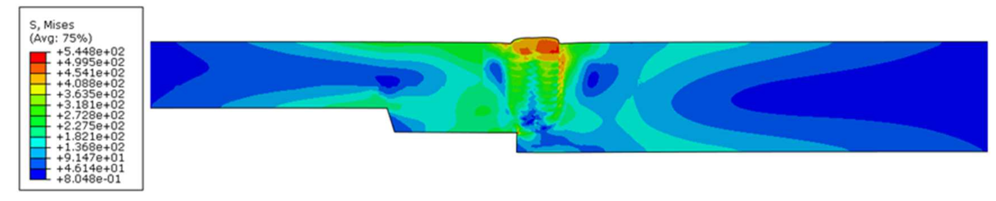
Figure 8.
FE prediction of von Mises stress (MPa) distribution in the DMW joint after girth welding.
Figure 9.
FE prediction of the radial (a), axial (b) and hoop (c) residual stress (MPa) distributions in the DMW joint after girth welding.
Figure 10.
FE prediction of von Mises stress (MPa) distribution in the DMW joint after machining.
Figure 11.
FE prediction of the radial (a), axial (b) and hoop (c) residual stress (MPa) distributions in the DMW joint after machining.
Figure 12.
Hoop residual stress (MPa) distribution obtained using the contour method: top—macrograph of the DMW joint, in which the cladding, buttering and the multi-pass girth weld areas are respectively marked with blue, red and black dotted lines; bottom—the contour plot of the hoop residual stress, in which the corresponding regions are also marked with dotted lines.
Figure 13.
Three paths defined along the neutron scan lines (refer to
Figure 4) across the DMW joint for residual stress evaluation and comparison.
Figure 14.
Comparison of hoop residual stresses along the three paths (as defined in
Figure 13) between the FE prediction and experimental measurements: (
a) along path 1 (near OD); (
b) along path 2 (mid-wall); (
c) along path 3 (near ID).
Table 1.
Materials used for the various parts of the mock-up.
| No. | Name | Material | Comments |
|---|
| 1 | Ferritic steel tube | SA508-3 | Forged and quenched + tempered |
| 2 | Stainless steel tube | 316L | Forged and solution treated |
| 3 | Clad layer | ER308L/ER309L | Filler metal |
| 4 | Flange | ERNiCrFe-7 | Inconel Welding Electrode 152 |
| 5 | Buttering layer | ERNiCrFe-7A | Inconel Filler Metal 52M |
| 6 | Girth weld | ERNiCrFe-7A | Inconel Filler Metal 52M |
Table 2.
Chemical composition of the ferritic steel tube.
| Element | C | Mn | Si | S | P | Cr | Ni | Cu | Mo | V |
|---|
| Specification | ≤0.25 | 1.20–1.50 | 0.15–0.40 | ≤0.005 | ≤0.015 | 0.10–0.25 | 0.40–1.00 | ≤0.15 | 0.45–0.60 | ≤0.05 |
| Actual | 0.17 | 1.48 | 0.25 | 0.003 | 0.007 | 0.18 | 0.96 | 0.05 | 0.47 | 0.001 |
Table 3.
Tensile properties of the ferritic steel tube.
| Property | Yield Strength (MPa) | Tensile Strength (MPa) | Elongation (%) | ROA (%) |
|---|
| Specification | ≥450 | 620–795 | ≥16 | ≥35 |
| Actual | 589 | 711 | 30 | 76 |
Table 4.
Chemical composition of the stainless steel tube.
| Element | C | Mn | Si | S | P | Cr | Ni | Co | Mo | N |
|---|
| Specification | ≤0.030 | ≤2.00 | ≤1.00 | ≤0.005 | ≤0.040 | 16.0–18.0 | 10.0–14.0 | ≤0.05 | 2.00–3.00 | 0.10–0.16 |
| Actual | 0.025 | 1.5 | 0.33 | 0.003 | 0.02 | 16.95 | 11.94 | 0.032 | 2.3 | 0.12 |
Table 5.
Tensile properties of the stainless steel tube.
| Property | Yield Strength (MPa) | Tensile Strength (MPa) | Elongation
(%) | ROA
(%) |
|---|
| Specification | ≥205 | ≥485 | ≥30 | ≥45 |
| Actual | 299 | 581 | 62 | 77 |
Table 6.
Welding process parameters used for each pass of the weld joint.
| Pass No./Layer No. | Pre-Heat/Inter-Layer Temp. (°C) | Peak/Base Current (A) | Peak/Base Voltage (V) | Welding Speed (mm/min) | Wire Feed Speed (mm/min) |
|---|
| 1/1 | 14/14 | 220/120 | 9.5 | 85 | 889 |
| 2/1 | 47/52 | 230/130 | 9.6 | 85 | 889 |
| 1/2 | 82/89 | 250/150 | 9.7 | 85 | 889 |
| 2/2 | 96/99 | 250/150 | 9.6 | 85 | 889 |
| 1/3 | 102/107 | 250/160 | 9.8 | 85 | 1143 |
| 2/3 | 117/120 | 260/160 | 9.6 | 85 | 1143 |
| 1/4 | 53/56 | 260/160 | 9.5 | 85 | 1143 |
| 2/4 | 74/89 | 260/160 | 9.6 | 85 | 1143 |
| 1/5 | 132/137 | 260/160 | 9.6 | 85 | 1143 |
| 2/5 | 18/18 | 260/160 | 9.7 | 85 | 1143 |
| 1/6 | 48/55 | 260/160 | 9.6 | 85 | 1143 |
| 2/6 | 78/89 | 260/160 | 9.5 | 85 | 1143 |
| 1/7 | 68/74 | 260/160 | 9.6 | 85 | 1143 |
| 2/7 | 102/107 | 260/160 | 9.7 | 85 | 1143 |
| 1/8 | 107/112 | 260/160 | 9.6 | 85 | 1143 |
| 2/8 | 110/116 | 260/160 | 9.5 | 85 | 1143 |
| 1/9 | 115/124 | 260/160 | 9.6 | 85 | 1143 |
| 2/9 | 120/127 | 260/160 | 9.6 | 85 | 1143 |
| 1/10 | 124/132 | 260/160 | 9.6 | 85 | 1143 |
| 2/10 | 128/138 | 260/160 | 9.6 | 85 | 1143 |
| 1/11 | 44/50 | 260/160 | 9.8 | 85 | 1143 |
| 2/11 | 48/66 | 260/160 | 9.8 | 85 | 1143 |
Table 7.
Elastic constants used for residual stress calculations.
| Elastic Constants | Fe-Alpha | Fe-Gamma | Nickel |
|---|
| E, GPa | 211 | 192 | 209 |
| v | 0.29 | 0.3 | 0.31 |
Table 8.
Thermo-physical properties data of SA508-3.
Temperature
(°C) | Density
(g/cm3) | Specific Heat
(kJ/kg/°C) | Thermal Conductivity
(W/m/°C) | Coefficient of Thermal Expansion
×10−6 (mm/mm/°C) | Young’s Modulus
(GPa) | Poisson’s Ratio |
|---|
| 25 | 7.85 | 0.450 | 41.0 | 12.5 | 210.9 | 0.289 |
| 100 | 7.83 | 0.481 | 41.8 | 12.7 | 207.1 | 0.292 |
| 200 | 7.80 | 0.520 | 41.7 | 13.1 | 201.8 | 0.296 |
| 300 | 7.77 | 0.564 | 40.5 | 13.5 | 193.9 | 0.300 |
| 400 | 7.73 | 0.618 | 38.6 | 13.8 | 184.1 | 0.304 |
| 500 | 7.70 | 0.688 | 36.3 | 14.2 | 172.3 | 0.308 |
| 600 | 7.66 | 0.786 | 34.0 | 14.6 | 159.1 | 0.311 |
| 700 | 7.64 | 1.131 | 29.8 | 13.8 | 142.2 | 0.322 |
| 800 | 7.66 | 0.594 | 26.0 | 11.0 | 127.5 | 0.339 |
| 900 | 7.60 | 0.609 | 27.3 | 12.5 | 117.7 | 0.345 |
| 1000 | 7.55 | 0.624 | 28.5 | 13.8 | 107.7 | 0.351 |
| 1100 | 7.50 | 0.640 | 29.7 | 14.9 | 97.6 | 0.357 |
| 1200 | 7.44 | 0.655 | 31.0 | 15.6 | 87.4 | 0.363 |
| 1300 | 7.39 | 0.671 | 32.2 | 16.4 | 77.0 | 0.369 |
| 1400 | 7.34 | 0.687 | 33.4 | 17.0 | 66.5 | 0.375 |
Table 9.
Flow stress of SA508-3 at different temperatures.
| Plastic Strain (%) | 0 | 4 | 8 | 12 | 16 | 20 | 24 | 28 |
|---|
| Temperature (°C) | True Stress (MPa) |
|---|
| 25 | 420 | 625 | 685 | 723 | 751 | 773 | 792 | 809 |
| 200 | 301 | 459 | 506 | 535 | 557 | 575 | 590 | 603 |
| 500 | 244 | 376 | 415 | 440 | 459 | 474 | 487 | 498 |
| 700 | 220 | 335 | 369 | 390 | 406 | 411 | 405 | 399 |
| 900 | 56 | 70 | 70 | 70 | 69 | 69 | 68 | 68 |
| 1100 | 26 | 26 | 26 | 26 | 26 | 26 | 26 | 25 |
| 1400 | 6.0 | 6.0 | 6.0 | 6.0 | 6.0 | 6.0 | 6.0 | 6.0 |
Table 10.
Thermo-physical properties data of 316L.
Temperature
(°C) | Density
(g/cm3) | Specific Heat
(kJ/kg/°C) | Thermal Conductivity
(W/m/°C) | Coefficient of Thermal Expansion
×10−6 (mm/mm/°C) | Young’s Modulus
(GPa) | Poisson’s Ratio |
|---|
| 25 | 7.99 | 0.447 | 13.67 | 18.85 | 194.3 | 0.298 |
| 100 | 7.96 | 0.468 | 14.67 | 18.99 | 189.2 | 0.301 |
| 200 | 7.92 | 0.489 | 16.00 | 19.20 | 182.2 | 0.306 |
| 300 | 7.87 | 0.507 | 17.34 | 19.42 | 175.0 | 0.310 |
| 400 | 7.82 | 0.524 | 18.68 | 19.65 | 167.8 | 0.315 |
| 500 | 7.77 | 0.540 | 20.01 | 19.89 | 160.4 | 0.319 |
| 600 | 7.73 | 0.557 | 21.35 | 20.13 | 152.8 | 0.324 |
| 700 | 7.68 | 0.574 | 22.69 | 20.38 | 145.2 | 0.328 |
| 800 | 7.63 | 0.592 | 24.02 | 20.65 | 137.4 | 0.333 |
| 900 | 7.58 | 0.610 | 25.36 | 20.92 | 129.4 | 0.337 |
| 1000 | 7.53 | 0.628 | 26.69 | 21.20 | 121.3 | 0.342 |
| 1100 | 7.48 | 0.648 | 28.03 | 21.50 | 113.1 | 0.346 |
| 1200 | 7.43 | 0.668 | 29.36 | 21.79 | 104.8 | 0.351 |
| 1300 | 7.37 | 0.688 | 30.70 | 22.09 | 96.3 | 0.355 |
| 1400 | 7.32 | 0.856 | 32.28 | 22.34 | 86.3 | 0.359 |
Table 11.
Flow stress of 316L at different temperatures.
| Plastic Strain (%) | 0 | 4 | 8.3 | 12.7 | 17.3 | 22.1 | 24.6 | 27.1 |
|---|
| Temperature (°C) | True Stress (MPa) |
|---|
| 25 | 362 | 613 | 671 | 697 | 707 | 708 | 707 | 704 |
| 200 | 265 | 507 | 571 | 602 | 618 | 625 | 626 | 626 |
| 500 | 219 | 426 | 481 | 508 | 523 | 529 | 531 | 531 |
| 700 | 207 | 373 | 414 | 433 | 441 | 444 | 444 | 443 |
| 900 | 153 | 147 | 141 | 135 | 129 | 123 | 119 | 116 |
| 1100 | 39 | 38 | 36 | 35 | 33 | 31 | 31 | 30 |
| 1400 | 6 | 6 | 6 | 6 | 6 | 6 | 6 | 6 |
Table 12.
Thermo-physical properties data of ER309L.
Temperature
(°C) | Density
(g/cm3) | Specific Heat
(kJ/kg/°C) | Thermal Conductivity
(W/m/°C) | Coefficient of Thermal Expansion
×10−6 (mm/mm/°C) | Young’s Modulus
(GPa) | Poisson’s Ratio |
|---|
| 25 | 7.94 | 0.449 | 13.80 | 18.4 | 193.8 | 0.299 |
| 100 | 7.90 | 0.470 | 14.79 | 18.6 | 188.8 | 0.302 |
| 200 | 7.86 | 0.492 | 16.11 | 18.8 | 181.9 | 0.306 |
| 300 | 7.81 | 0.510 | 17.43 | 19.1 | 174.9 | 0.311 |
| 400 | 7.77 | 0.527 | 18.75 | 19.3 | 167.7 | 0.315 |
| 500 | 7.72 | 0.544 | 20.07 | 19.6 | 160.3 | 0.319 |
| 600 | 7.67 | 0.561 | 21.39 | 19.8 | 152.8 | 0.324 |
| 700 | 7.63 | 0.629 | 22.70 | 20.1 | 145.1 | 0.328 |
| 800 | 7.58 | 0.608 | 24.34 | 20.5 | 136.0 | 0.333 |
| 900 | 7.52 | 0.616 | 25.68 | 20.9 | 128.0 | 0.337 |
| 1000 | 7.47 | 0.635 | 27.02 | 21.2 | 120.0 | 0.341 |
| 1100 | 7.42 | 0.655 | 28.36 | 21.5 | 112.0 | 0.346 |
| 1200 | 7.37 | 0.676 | 29.70 | 21.8 | 103.9 | 0.350 |
| 1300 | 7.32 | 0.698 | 31.03 | 22.1 | 95.5 | 0.354 |
| 1400 | 7.27 | 0.849 | 32.79 | 22.3 | 84.2 | 0.358 |
Table 13.
Flow stress of ER309L at different temperatures.
| Plastic Strain (%) | 0 | 4 | 8 | 12 | 16 | 20 | 24 | 28 |
|---|
| Temperature (°C) | True Stress (MPa) |
|---|
| 25 | 383 | 574 | 631 | 666 | 692 | 714 | 731 | 747 |
| 200 | 273 | 418 | 462 | 489 | 510 | 526 | 540 | 552 |
| 500 | 221 | 343 | 380 | 403 | 420 | 434 | 445 | 455 |
| 700 | 132 | 132 | 131 | 130 | 128 | 126 | 125 | 124 |
| 900 | 24 | 24 | 24 | 23 | 23 | 23 | 22 | 22 |
| 1100 | 6.5 | 6.5 | 6.5 | 6.4 | 6.3 | 6.2 | 6.1 | 6.1 |
| 1400 | 1.5 | 1.4 | 1.4 | 1.4 | 1.4 | 1.4 | 1.4 | 1.4 |
Table 14.
Thermo-physical properties data of INCONEL52M.
Temperature
(°C) | Density
(g/cm3) | Specific Heat
(kJ/kg/°C) | Thermal Conductivity
(W/m/°C) | Coefficient of Thermal Expansion
×10−6 (mm/mm/°C) | Young’s Modulus
(GPa) | Poisson’s Ratio |
|---|
| 25 | 8.19 | 0.435 | 13.03 | 12.35 | 214.3 | 0.311 |
| 100 | 8.17 | 0.452 | 14.34 | 12.68 | 209.5 | 0.313 |
| 200 | 8.14 | 0.470 | 16.07 | 13.14 | 202.8 | 0.317 |
| 300 | 8.10 | 0.488 | 17.79 | 13.60 | 195.8 | 0.320 |
| 400 | 8.07 | 0.505 | 19.49 | 14.06 | 188.6 | 0.323 |
| 500 | 8.03 | 0.522 | 21.17 | 14.51 | 181.2 | 0.327 |
| 600 | 7.99 | 0.666 | 22.84 | 14.96 | 173.5 | 0.330 |
| 700 | 7.94 | 0.708 | 23.23 | 15.83 | 162.7 | 0.332 |
| 800 | 7.89 | 0.581 | 23.98 | 16.68 | 152.0 | 0.333 |
| 900 | 7.84 | 0.604 | 25.54 | 17.15 | 143.6 | 0.336 |
| 1000 | 7.79 | 0.629 | 27.09 | 17.64 | 134.8 | 0.339 |
| 1100 | 7.74 | 0.644 | 28.64 | 18.13 | 125.8 | 0.342 |
| 1200 | 7.69 | 0.668 | 30.20 | 18.62 | 116.7 | 0.345 |
| 1300 | 7.64 | 0.693 | 31.76 | 19.11 | 107.4 | 0.348 |
Table 15.
Flow stress of INCONEL52M at different temperatures.
| Plastic Strain (%) | 0 | 4 | 8 | 12 | 16 | 20 | 24 | 28 |
|---|
| Temperature (°C) | True Stress (MPa) |
|---|
| 25 | 361 | 637 | 726 | 784 | 828 | 864 | 894 | 920 |
| 200 | 277 | 545 | 637 | 698 | 745 | 784 | 816 | 845 |
| 500 | 240 | 476 | 556 | 609 | 650 | 684 | 713 | 739 |
| 700 | 229 | 407 | 407 | 406 | 405 | 402 | 399 | 396 |
| 900 | 92 | 92 | 92 | 92 | 92 | 92 | 91 | 90 |
| 1100 | 25 | 25 | 25 | 25 | 25 | 25 | 24 | 24 |
| 1300 | 8 | 8 | 8 | 8 | 8 | 8 | 8 | 8 |
Table 16.
Reduction of maximum weld residual stresses due to machining.
| Residual Stress | Condition | Reduction Due to Machining, % |
|---|
| As-Welded | After Machining |
|---|
| von Mises, MPa | 544.8 | 427.4 | 21.5 |
| Radial, MPa | 576.1 | 134.8 | 76.6 |
| Axial, MPa | 545.3 | 242.2 | 55.6 |
| Hoop, MPa | 757.5 | 467.7 | 38.3 |
| Publisher’s Note: MDPI stays neutral with regard to jurisdictional claims in published maps and institutional affiliations. |
© 2021 by the authors. Licensee MDPI, Basel, Switzerland. This article is an open access article distributed under the terms and conditions of the Creative Commons Attribution (CC BY) license (https://creativecommons.org/licenses/by/4.0/).


 ,
, 


