Development of a Fast Modeling Approach for the Prediction of Scrap Preheating in Continuously Charged Metallurgical Recycling Processes

Abstract

Improving the overall energy efficiency of processes is necessary to reduce costs, lower the specific energy consumption and thereby reduce the direct or indirect emission of gases that contribute to climate change. In many metallurgical processes, a large amount of energy is lost with the off-gas. In metallurgical recycling processes, off-gas often can be used to preheat the to-be-recycled metal scrap, leading to significantly higher energy efficiency. However, the application of preheating has the disadvantage that it often requires more precise planning in the design and better control of the process. In this paper, a simplified look at a continuously charged scrap preheating aggregate for the widely used electric arc furnace (EAF) in the steel processing industry is used as illustration. Continuous scrap charging in EAF-type furnaces in general has much higher demands on process control and general process knowledge, which is why they are found only very rarely. General issues and basic modeling approaches to mitigate such issues allowing a better process control will be described. In particular, a fast, one-dimensional modeling approach for the determination of the temperature distribution inside a constantly moving scrap bulk, with hot air (or exhaust gases) flowing through it, will be described. Possible modeling applications, assumptions, possible enhancements and limitations are shown. The first results indicate that this approach can be used as a solid basis for the modeling of scrap bulks with thermally thin parts, consisting of materials with similar thermodynamic material properties. Therefore, as a basis, this approach may help improve the design and control of future or existing preheating devices in metal recycling processes.

1. Introduction

Making better use of waste energy, usually in the form of heat, is necessary to increase the energy efficiency of nearly every process. A large amount of such waste heat, for example, occurring in recycling metallurgical melting processes, is often lost within the off-gas. Today, recycling processes are very important due to their overall better energy efficiency. To give an example, the steel production from recycled materials saves about 1.5 tons of CO₂ per ton of steel, saving around 945 million tons of CO₂ emissions per year [1], not to mention the significant damages to the environment induced by primary iron ore or coal mining. It is estimated that roughly 630 million tons of steel are produced from recycled material every year, with increasing tendency [1]. The most relevant process for steel recycling is the electric arc furnace process. Furthermore, with CO₂-neutral primary iron production processes such as direct reduced iron (DRI), the importance of the electric arc furnace will continue to increase, as it is also required in this process chain. Therefore, further improving its efficiency is very relevant to decrease the worldwide CO₂ emissions; it is also a good investment in the foreseeable future. In the EAF process, a large amount of the supplied energy (approximately 30% [2]) is lost within the off-gas, whose temperature ranges between 750 and 1200 °C, depending on the process and point of measurement. According to Nardin et al. [2], there are many strategies for making better use of the waste energy especially in this kind of process. One strategy is clearly obvious, namely, to use the energy of the off-gas for preheating of the charged material, which can be assigned under direct heat recovery techniques. Thereby, the enthalpy of the charged material is increased, and the heat required for melting the scrap inside the metal bath is reduced. So why is this not the common practice by now? Of course, there are some drawbacks introduced by this approach which only can be surpassed via good process control. For example, according to Toulouevski and Zinorov [3], a maximum temperature between 1560 and 1580 °C must be held inside the metal bath to prevent excessive refractory wear. This is only around 50 °C above liquidus temperature. Furthermore, the heat transfer between molten metal and scrap is limited due to the low convection speeds inside the melt. Since the scrap cannot be homogeneously charged across the liquid bath and a continuous charging between the hot spot inside the melt, between the electrodes, is difficult from a constructive point of view, the temperature and mass flow rate of scrap that is charged must be strictly controlled. Additionally, the off-gas has to undergo some post combustion process to remove CO and lower NO_x. A sensible approach is to split the off-gas between a scrap preheating device and another off-gas channel and bring them back together later for post combustion. Therefore, it is important that the mixed off-gas still has enough energy in combination with some mixed-in air that post-combustion is still possible. At least, it should still have enough energy, so that only little energy, for example, from a post combustion burner, must be added. Otherwise, scrap preheating would not be very effective. In addition, due to organic residues on the scrap, there are usually increased dioxin emissions when preheating techniques are applied [4,5]. The dioxin amount in the off-gas can be reduced, but to achieve this in a cost and energy efficient way, a relatively high temperature (above 850 °C) has to be maintained in the post-combustion chamber, followed by a quick cooling step between 600 and 200 °C to avoid reformation of dioxins [6]. To keep the described problems and the dynamic interactions between the individual problems under control, a significantly improved process control is required. Here, different modeling techniques can be used to better understand, plan and later better control those process interactions between preheating, off-gas temperature and bath temperature.

There have been several publications of concepts, patents and other materials for continuous preheating concepts in the recent years [7,8,9,10]. In the latest literature, CFD models and process models regarding the topic of scrap preheating can be found [11,12,13,14,15], but they either lack a detailed description of the model, the simplification level is too high (for example lacking a prediction of the temperature distribution in the bulk) or these approaches are too computationally intensive to be used to build online control models. Zhang and Oeters [16] described a similar modeling approach as in this paper, with the additional modeling of some chemical reactions, but for a different application.

In this paper a basic, fast and also extensible 1D modeling approach for the preheating of flown through bulk material is described. As an example, for relevant application, a simplified view on a continuously charged EAF is presented. In particular, we refer to the so-called ISMELT^® technology, recently developed by Inteco Inc. (Bruck an der Mur, Austria) [10], and use it as an illustrative example. In this paper, the modeling will focus on the prediction of the scrap preheating and the cooling of the off-gas. In the future, the model can be used to be coupled with more general EAF models, for example, as described by Hay et al. [17] to predict the overall modified process behavior. Furthermore, thanks to its simplicity and the implementation with the Julia programming language, with its powerful dispatch model [18,19], it is extensible, fast, versatile and may help to further develop suitable online control models.

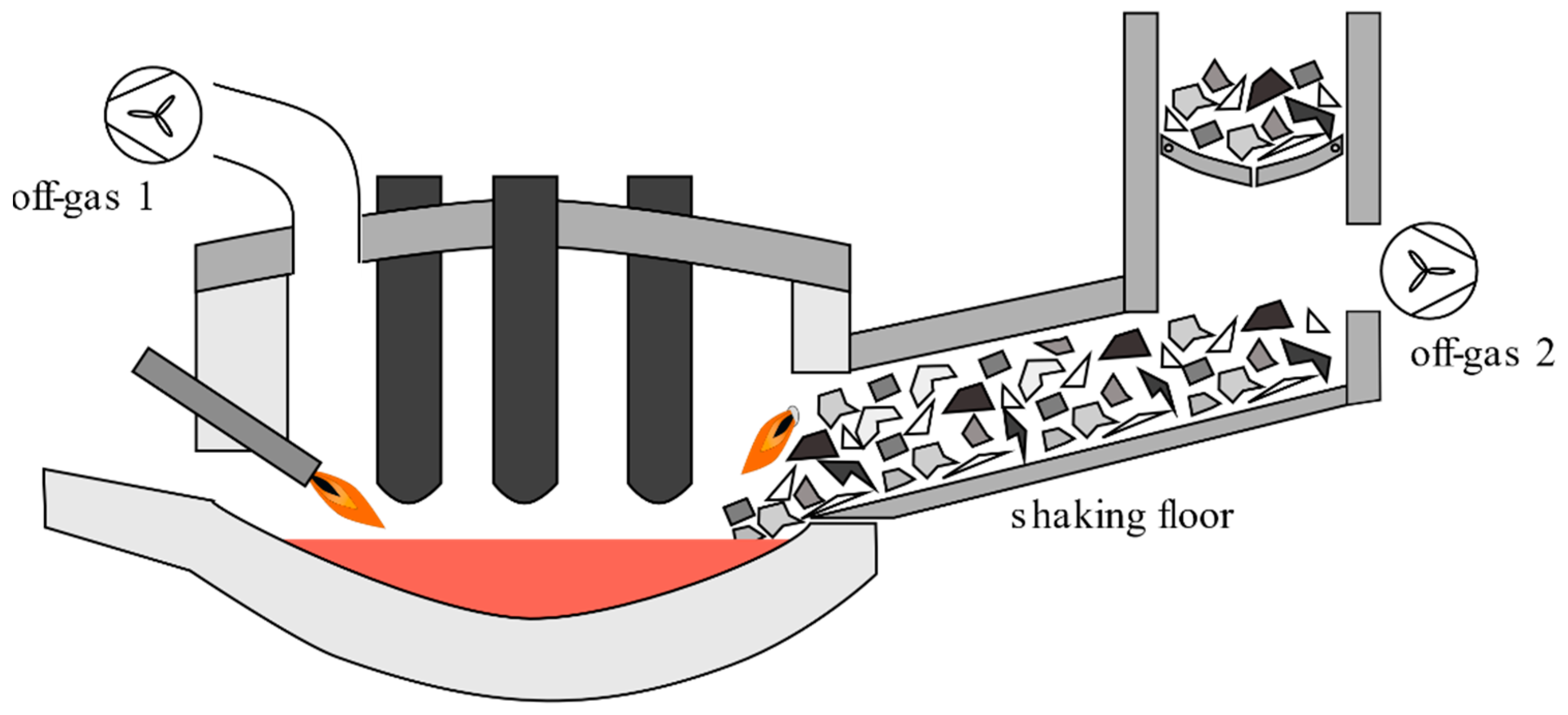
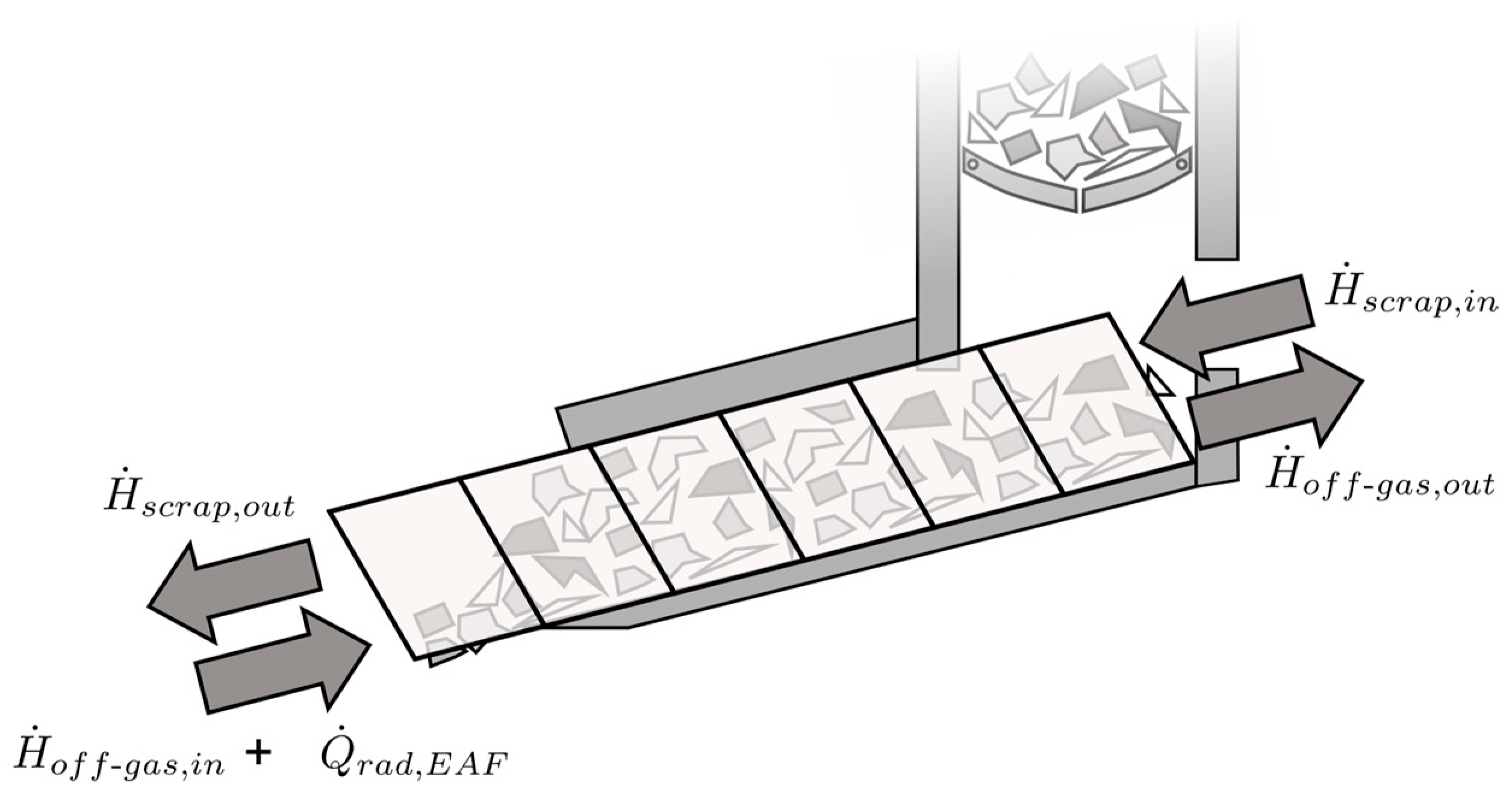
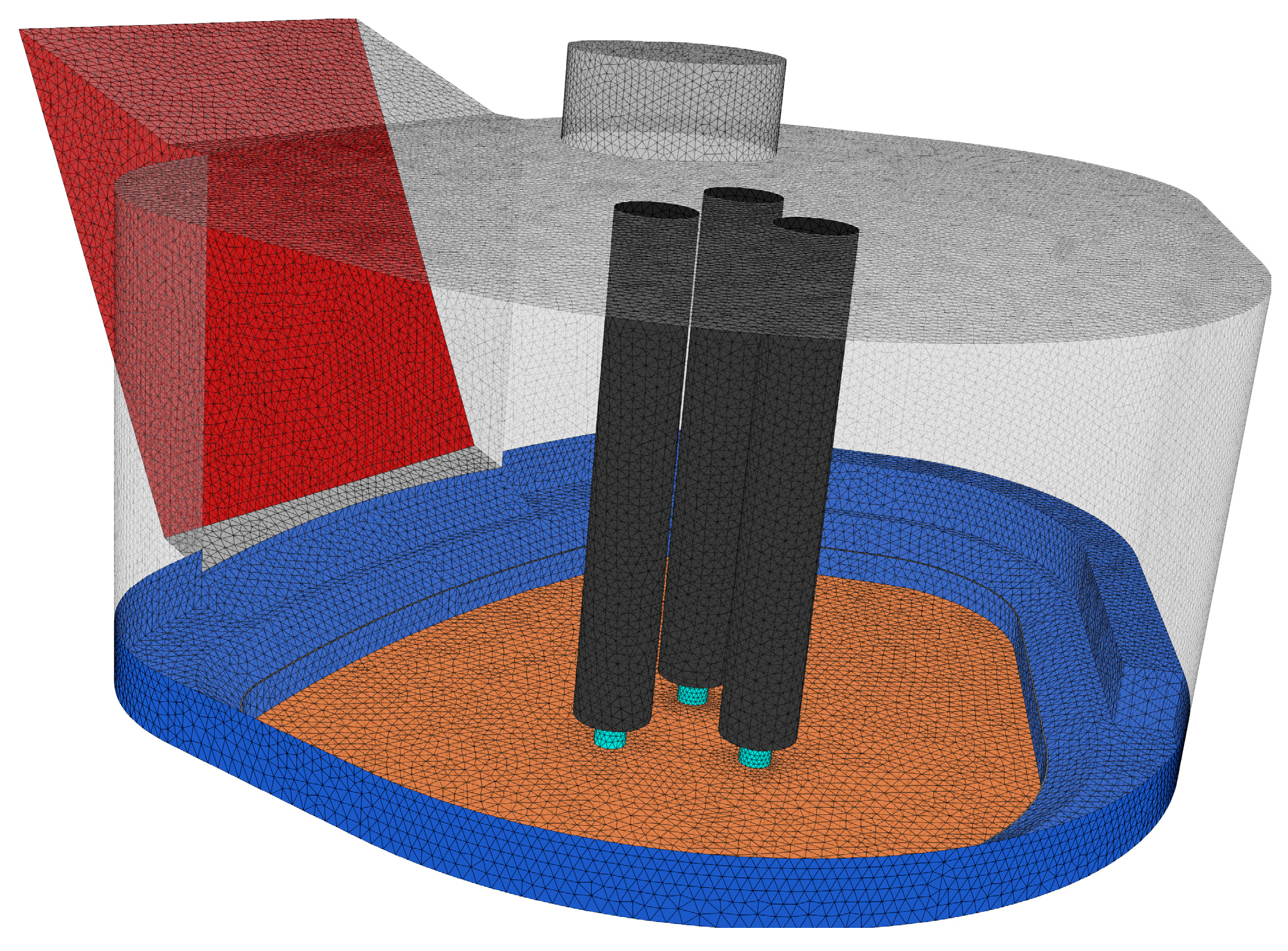
Description of the Modeled Process

The illustrative process is shown in Figure 1. The scrap is charged into an inclined shaft with some sort of transportation support and control mechanism, for example, a shaking floor, at the side of the EAF. The off-gas can be controlled to be distributed between the shaft and the usual EAF off-gas exhaust. As already described, this is necessary, since the two off-gas flows will be mixed again for post combustion of organic components and purification.

Although it is called continuous scrap charging, the EAF process is inherently a batch process with multiple process phases. A continuously charged EAF process should be run in two phases [3]. First, the flat-bath melting phase, and second, the refining phase. During the more or less continuous flat-bath melting phase, the scrap is continuously charged into the residual melt remaining from the previous tapping. During the refining phase, the charging of scrap is stopped and the slag layer above the hot melt is broken up by the now activated oxygen lances, thus, a higher amount of thermal radiation from the melt and electric arcs reaches the scrap in front of the shaft, and since charging is stopped, the scrap bulk is standing still in the charging shaft. Therefore, there is a higher risk that partial melting of scrap parts may occur. This could potentially block scrap charging by clumping or damaging the charging mechanism. To evaluate the possibility of such behavior, simplified modeling approaches for the two phases under the following assumptions are used:

• Flat-bath melting phase model (phase 1): Here, a continuous scrap flow to the melt is modeled. The off-gas temperature and flow rate is assumed to be constant.
• Refining phase (phase 2): No off-gas or scrap flow through the shaking floor tunnel, heat transfer inside the scrap bulk is mainly driven by surface to surface (s2s) radiation effects.

The flat-bath melting phase is assumed to last around 50 min, while the refining phase is assumed to last around 5 min.

2. Materials and Modeling Approach

2.1. Materials

2.1.1. Scrap

The assumption about size distribution and material properties of scrap material has great influence on the following investigations. Therefore, the scrap material is a main interest for this study. There are different implications of the scrap material to the process. The main influences of the scrap material to the process behavior are:

• Scrap composition (steel grades and alloying elements);
• Scrap contamination in terms of adherent organic materials;
• Distribution of the geometrical characteristics of the scrap speaking of the mean scrap part thickness and the surface to volume ratio.

All these unknowns can influence the scrap preheating temperature, the off-gas composition or the pressure loss curve over the length of the preheating shaft. The pressure loss over the length of the shaft is very important, because it must be compensated for to define a controlled volume flow through the shaft. As there is no general information about the consistency of the scrap available, which also may change from charge to charge, some simplifying assumptions will be used for now. Once, it is assumed that the scrap steel uniformly consists of steel 1.0035, with a high Fe amount of 99%, as given by the European steel register [20]. The density is given with a constant value of 7850 kg/m³; the other properties are shown in Figure 2.

Furthermore, it is assumed that the smallest pieces of scrap will have the most significant influence on the pressure loss over the scrap itself. Therefore, three different characteristic scrap sizes listed in

Table 1. Different scrap classes.

Name	Label	Density in kg/m³	Dimensions (Length × Width × Thickness) in m	Source
Turning chips	S1	500	0.25 × 0.03 × 0.001	Measurements from CNC scrap of our workshop
Rail crops scrap	S2	1121	1.21 × 0.45 × 0.0127	Datasheet [21]
Plate Scrap	S3	801	0.92 × 0.61 × 0.003175	Datasheet [21]

will be used for the further investigations.

2.1.2. Off-Gas

As for the scrap, there will be some very significant simplifications used for the off-gas. The composition will be assumed with a (constant) composition of 70 vol.-% N₂, 10 vol.-CO₂ and 20 vol.-% CO, as roughly approximated from the flat-bath melting phase of comparable sized EAF processes. The temperature-dependent material properties were calculated with Cantera [22] using the GRI-Mech 3.0 thermodynamic mechanism set [23]. The properties are shown in Figure 3.

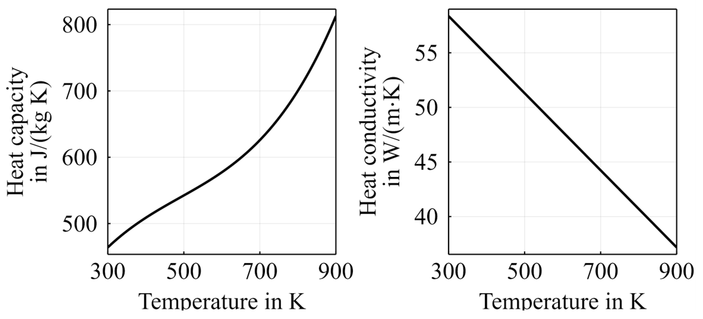
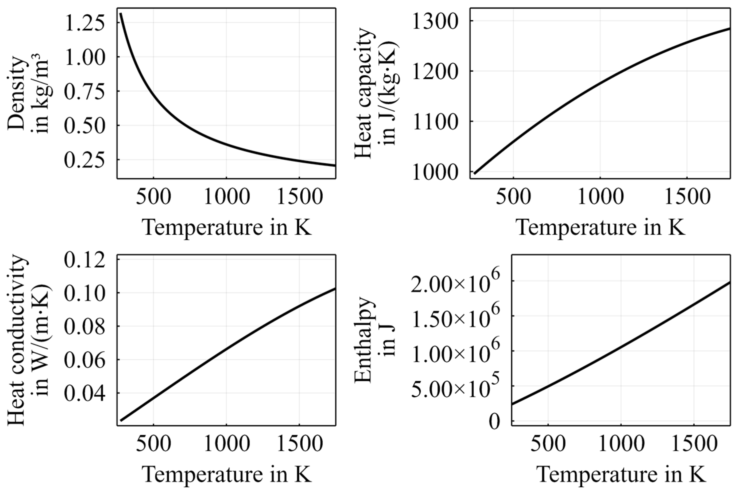
2.2. Modeling Parameters

A crucial point for the model’s predictive power is the appropriate choice of different model parameters, such as characteristic surface areas or characteristic lengths. These parameters are roughly estimated within this work, as can be seen in

Table 2. Operating data for modeled scrap bulk shaft.

Property	Value	Unit
Input temperature scrap	25	°C
Mass flow scrap	38.6	kg/s
Mass flow off-gas (through scrap bulk)	6.64	kg/s
Floor length	8	m
Floor cross section area	2.9 × 3.2	m²

, but could also be more exactly defined using more detailed investigations or automated modeling optimizing techniques, when combined with real operation data.

2.3. Modeling Approach

The model is essentially developed combining two or three one-dimensional energy transports models, namely, over the fluid phase, over the solid bulk phase and optionally over the individual scrap part’s thickness. The implementation itself is carried out using the Julia programming language (ver. 1.6) [18], it can be accessed in the Supplementary File S1. The model, furthermore, is derived using a fixed grid enthalpy-based, energy balance modeling approach, including the capability to include temperature dependent material properties of the off-gas and the scrap material.

Therefore, the shaking floor tunnel is virtually divided into separate cross section layers (bulk layers), perpendicular to flow or scrap movement, as can be seen in Figure 4. Each layer in this discretized bulk volume is then again divided into one off-gas cell and 1 to $n_j$ multiple scrap layer cells, which can be seen in Figure 5. These scrap layer cells, if more than one is used, will model the heat conduction in an exemplary scrap piece of the bulk at the position $i$. Considering the thickness of the scrap parts may be relevant if they are thermally thick, which usually is the case if the Biot number $Bi$, Equation (1), is greater than 0.1. Here, $\alpha$ is the heat transfer coefficient, $l_{char}$ is the characteristic thickness of the material and ${\lambda }_s$ its thermal conductivity. Here, this approach also allows for some optional approximation of the thermal distribution inside the scrap, under the assumption that the scrap parts can be sufficiently characterized using one characteristic thickness and a representative surface. Therefore, this approach may also be referred to as the 1D(–1D) model.

$$Bi=\frac{\alpha \cdot l_{char}}{{\lambda }_s}$$

(1)

Following the notation in Figure 5, in the following text the cells in the $i$th direction will be referred to as bulk layer cells and the cells in $j$th direction as scrap layer cells. Each direction is discretized using homogeneous cell sizes.

In this model mass flow, convective, conductive and radiative heat transfer are expressed as incremental changes in the cell’s enthalpy, as isobaric process conditions can be assumed for this case. For the solver implementation, a $\mathrm{d}T/\mathrm{d}t$ formation is used, which is spatially discretized, to transform the PDE system into an ODE system. The “DifferentialEquations.jl” solver package [24] will be used for the solution of the resulting ODE system. For simplicity, the expressions will be written as change in enthalpy $\mathsf{\Delta }H$, which should facilitate the reading of the equations.

For example, the change in enthalpy, during a defined timestep $\mathsf{\Delta }t$ of the off-gas (fluid $f$) in each cell $i$, $\mathsf{\Delta }{H}_{i,f}$ can be expressed due to the off-gas mass flow ${\dot{m}}_f$ using Equation (2). $c_p$ is the true heat capacity.

$$\mathsf{\Delta }{H}_{i,f}={\dot{m}}_f\cdot \mathsf{\Delta }t{\int }_{T_{f,i-1}}^{T_{f,i}}{c}_{p,f}\mathrm{dT}$$

(2)

In the same way, it is possible to account for the scrap movement; as for the numerical approximation, it is sensible to use upwind approaches according to the movement direction the evaluation direction is flipped for the scrap cells (see Equation (3)).

$$\mathsf{\Delta }{H}_{i,s}={\dot{m}}_s\cdot \mathsf{\Delta }t{\int }_{T_{s,i}}^{T_{s,i+1}}{c}_{p,s}\mathrm{dT}$$

(3)

Furthermore, the enthalpy change due to heat transfer between all the scrap cells can be expressed within the $i$- and $j$-direction. The different heat transfer mechanisms are heat conduction within the scrap parts, heat conduction within contact areas between the scrap parts, convection between scrap and air and thermal radiation heat transport from the furnace side to the scrap and between individual scrap parts.

2.3.1. Modeling Simplifications

The current implementation of the model comes in hand with some simplifying assumptions; these assumptions are presented for better comprehensibility of the model:

• Scrap consisting of small flat stripes of metal with a characteristic thickness (which should translate to the fact that they have only one direction where thermal conduction will matter the most) and a representative surface area;
• All scrap parts are composed of the same material;
• Scrap pieces are shaped approximately equal and distributed evenly over the scrap bulk;
• The scrap bulk has uniform scrap thicknesses and constant surface to volume ratio;
• There is a uniform scrap movement in direction of the shaking floor;
• Neglection of gas radiation (the usual distance between different parts) is estimated to be in between 1 and 15 cm, and the gray gas emissivity for the given gas composition (over a temperature range from 300 K to 1500 K at 1 atm) varies between 0.01 and 0.08, calculated according to Alberti et al. [25]; therefore, its influence will be neglected for now);
• The emissivity of all surfaces (scrap and furnace walls) will be assumed to be 0.8;
• Assuming temperatures listed in

  Table 3. Temperatures for the calculation of ${\dot{Q}}_{rad,EAF}$ during phase 2 (geometry is shown in Figure 6).

  Color	Red	Blue	Cyan	Orange	Gray
  Temperature in °C	Modeled	1500	4500	1650	900

  for modeling of scrap bulk incident radiation for the refining phase (2);
• Neglecting dissipation and compressible pressure effects in the off-gas flow;
• Constant gas composition over whole process time;
• Constant heat transfer coefficient between scrap and off-gas over the length of the shaft;
• Symmetry assumption over the individual scrap part’s thicknesses;
• Neglecting the contact of scrap with the surrounding walls;
• No modeling of thermal conduction between the individual scrap parts in the bulk (convective and/or radiative heating is assumed to dominate the heat distribution of the scrap bulk);
• Homogeneous temperature and mass flow of the off-gas in each bulk layer cell.

2.3.2. Heat Conduction over Characteristic Scrap Thickness

First, the heat transfer through heat conduction in an individual (representative scrap piece), as shown in the lower part of Figure 5, will be modeled. The heat conduction term over the characteristic thickness of the scrap piece can be described using Equation (4). Here, $\mathsf{\Delta }{y}_s$ is the thickness of each scrap cell (index $s$) in $j$-direction, $A_{y, s}$ is the characteristic cross section surface of a scrap piece, normal to the main heat conduction direction.

$$\mathsf{\Delta }{H}_{i,j,s}=\mathsf{\Delta }t\cdot \frac{{\lambda }_{y,s}\left(T_{i,j,s}\right)}{\mathsf{\Delta }{y}_s}\cdot A_{y,s}\cdot \left(T_{i,j+1,s}+2 T_{i,j,s}-T_{i,j-1,s}\right)$$

(4)

2.3.3. Heat Conduction in the Off-Gas

Accordingly, the off-gas conduction in $i$ direction can be modeled using Equation (5), which may become relevant for very low off-gas flow rates. $\mathsf{\Delta }{x}_f$ is the length of the fluid cells (index $f$) in $i$-direction; in the current approach, the fluid and solid cells are overlaying each other, and $\mathsf{\Delta }{x}_f$ is equal to $\mathsf{\Delta }{x}_s$.

$$\mathsf{\Delta }{H}_{i,j,f}=\mathsf{\Delta }t\cdot \frac{{\lambda }_{x,f}\left(T_{i,j,f}\right)}{\mathsf{\Delta }{x}_f}\cdot A_f\cdot \left(T_{i+1,f}+2 T_{i,f}-T_{i-1,f}\right)$$

(5)

However, it its more difficult to come up with a simple model for the conductive heat transfer between the individual pieces and its resulting heat conduction contribution in $i$ direction over the scrap bulk.

2.3.4. Convective Heat Exchange between Scrap and Off-Gas

The energy transfer between the off-gas (fluid) and scrap (solid) models is realized using Equation (6). To also model the heat transfer in the case of no off-gas flow, a minimum value of ${\alpha }_{fs}$ of 10 W/(m² K) should be used. Using Equation (6), the change in the solid cell enthalpy through convective heat transfer is calculated as the product of heat transfer coefficient ${\alpha }_{fs}$ the scrap surface $A_{fs}$ and the difference between scrap $T_s$ and fluid (off-gas) $T_f$ temperature.

$$\delta Q_{i,fs}=\mathsf{\Delta }t\cdot {\alpha }_{fs}\cdot A_{fs}\cdot \left(T_{i,f}-T_{i,1,s}\right)$$

(6)

Here, the interfacial scrap surface $A_{fs}$ can be related to a hypothetical inter-facial area density $SA:V_b$, which represents the ratio of scrap surface m² to scrap volume in m³ in the bulk, and $A_{fs}=SA:V_b\cdot V_{fs}$, $SA:V_b$ can be calculated using the dimensions (distribution) of the scrap pieces, the summed overlapping contact area of the scrap pieces in m² per m³ and the density of the scrap bulk itself.

2.3.5. Balancing

The modeling of the radiation phenomena onto $\delta Q_{rad,i,front}$ and inside $\delta Q_{rad,i,cross}$ the scrap bulk is described in a separate section below.

Based on the summed balance of the different heat $Q$ and enthalpy $H$ changes, generally termed $\mathsf{\Delta }H$, the new temperature of each cell can be calculated, using the inverse function $T\left(H\right)$ of the enthalpy curve $H\left(T\right)$ of the given material, resulting in Equation (7). Here, $H\left(t\right)$ is the specific enthalpy of a cell at time $t$ and $m_{i,\left(j\right)}$ is the mass of the cell.

$$T_{t+\mathsf{\Delta }t}=T\left(H\left(t\right)+\frac{\sum \mathsf{\Delta }H}{m_{i,\left(j\right)}}\right)$$

(7)

2.3.6. Radiation Modeling—Bulk Incident Radiation

During the flat-bath melting phase (phase 1), it will be assumed that the off-gas is very dusty and gas radiation dominates, so Equation (8) is used to calculate the radiative heat transfer from the EAF environment to the front of the scrap bulk. Here, $A_{s,front}$ is the surface of the inclined front (Figure 6), with 16.4 m² and ${ϵ}_s$ is the emissivity of the scrap. This equation is then completed by introducing Equation (14), which takes the possible radiation transmittance of the first layer(s) into account.

$${\dot{Q}}_{i,rad,EAF}=\sigma \cdot {ϵ}_s\cdot A_{s,front}\cdot \left(T_i^4-T_{\infty , EAF}^4\right)$$

(8)

During the refining phase of the exemplary process, thermal surface to surface radiation effects will become the most important mechanisms between the individual scrap parts inside and onto the scrap bulk. Gas radiation effects, on the other hand, will be negligible (in the bulk itself), since the radiation distances between the individual parts are small and the overall heat capacity of the off-gas is low compared to the scrap’s heat capacity.

In particular, during the second (refining) phase of the exemplary continuously charged EAF process, where the scrap charging and the off-gas suction through the shaking floor tunnel will be stopped, thermal radiation effects onto and inside the scrap bulk will become highly relevant for the thermal distribution inside the scrap bulk. Therefore, the furnace’s scrap bulk temperature in front of the shaking floor may rise a lot more due to the incident thermal radiation.

To describe these radiation effects to the front of the scrap bulk, the surface to surface (s2s) approach is used. According to Hottel or Howel [26,27], the heat flow between thermal radiating surfaces to a special surface $i$ can be computed by Equation (9), which represent, the difference between the in- and outgoing heat fluxes $\dot{q}″$ multiplied with the radiation exchange surface area $A_i$ of a surface $i$.

$${\dot{Q}}_i=\left({\dot{q}}_{out,i }^{″}-{\dot{q}}_{in,i }^{″}\right)\cdot A_i$$

(9)

The outgoing heat flux can be evaluated solving the following linear equation system (10), if the geometry specific view factors $F_{ik}$ of the $N$ surfaces are known.

$$\left[{\displaystyle \sum }_k^N\left(ϵ-1\right)\cdot F_{ik}+{\delta }_{ik}\right]\cdot \left[{\dot{q}}_{out,i}^{″}\right]=\left[{ϵ}_i \sigma T_i^4\right]$$

(10)

To then calculate the surface incident heat flux ${\dot{q}}_{in,i }^{″}$, Equation (11) can be used.

$${\dot{q}}_{in,i }^{″}={\displaystyle \sum }_{k=1}^N{\dot{q}}_{out,k }^{″}\cdot F_{ik}$$

(11)

Using this approach, the heat flow ${\dot{Q}}_{rad,EAF}$ (Figure 4) to an area representing the front surface of the scrap bulk is calculated to include the furnace incident radiation effects inside the model. Therefore, the view factor matrix was calculated using an in-house radiation model. The geometry for the view factor calculation is shown in Figure 6.

For the differently colored faces, the temperatures given in Table 3 were assumed. Here, especially the assumed arc temperature (cyan) can vary a lot between different models (<2000–30,000 K) [28,29,30]. With a view factor of <1%, the impact of this temperature to the scrap front is not very important. Here, the shown values must be seen as a rough approximation that have no particular significance or are supported by measurement data. Nevertheless, to model an existing preheating process, those temperature assumptions must be optimized against existing process data, as these are highly relevant for the heat input over the refining phase 2.

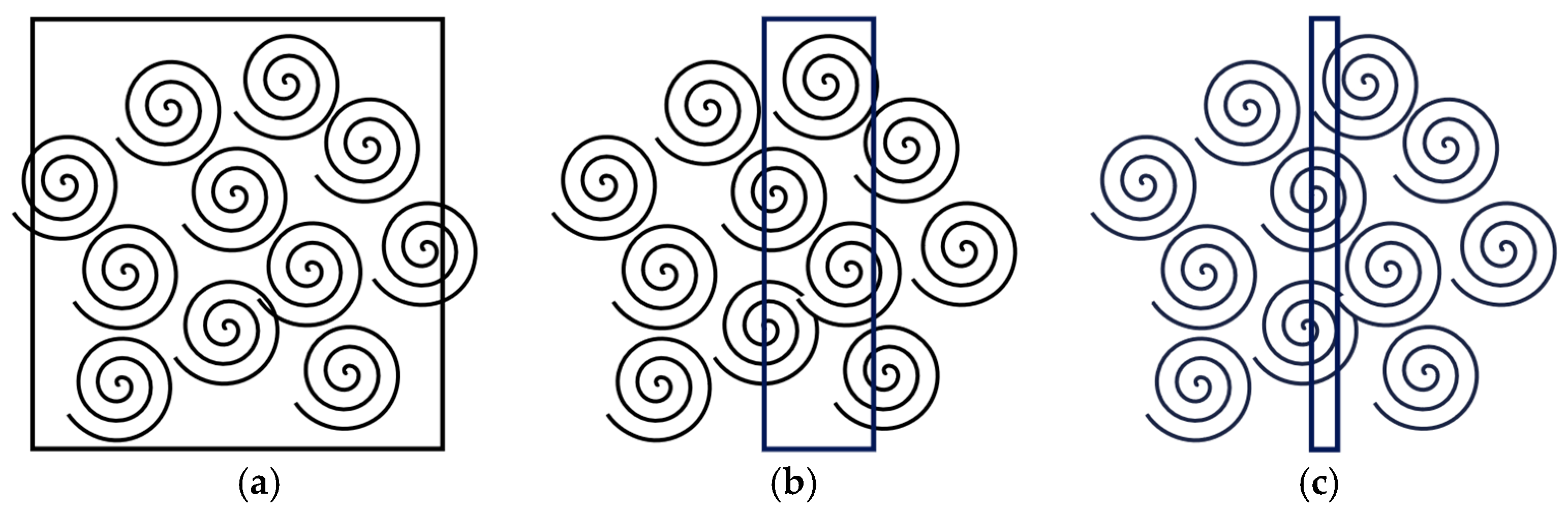
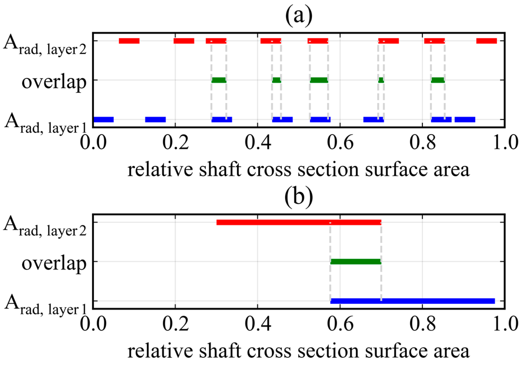
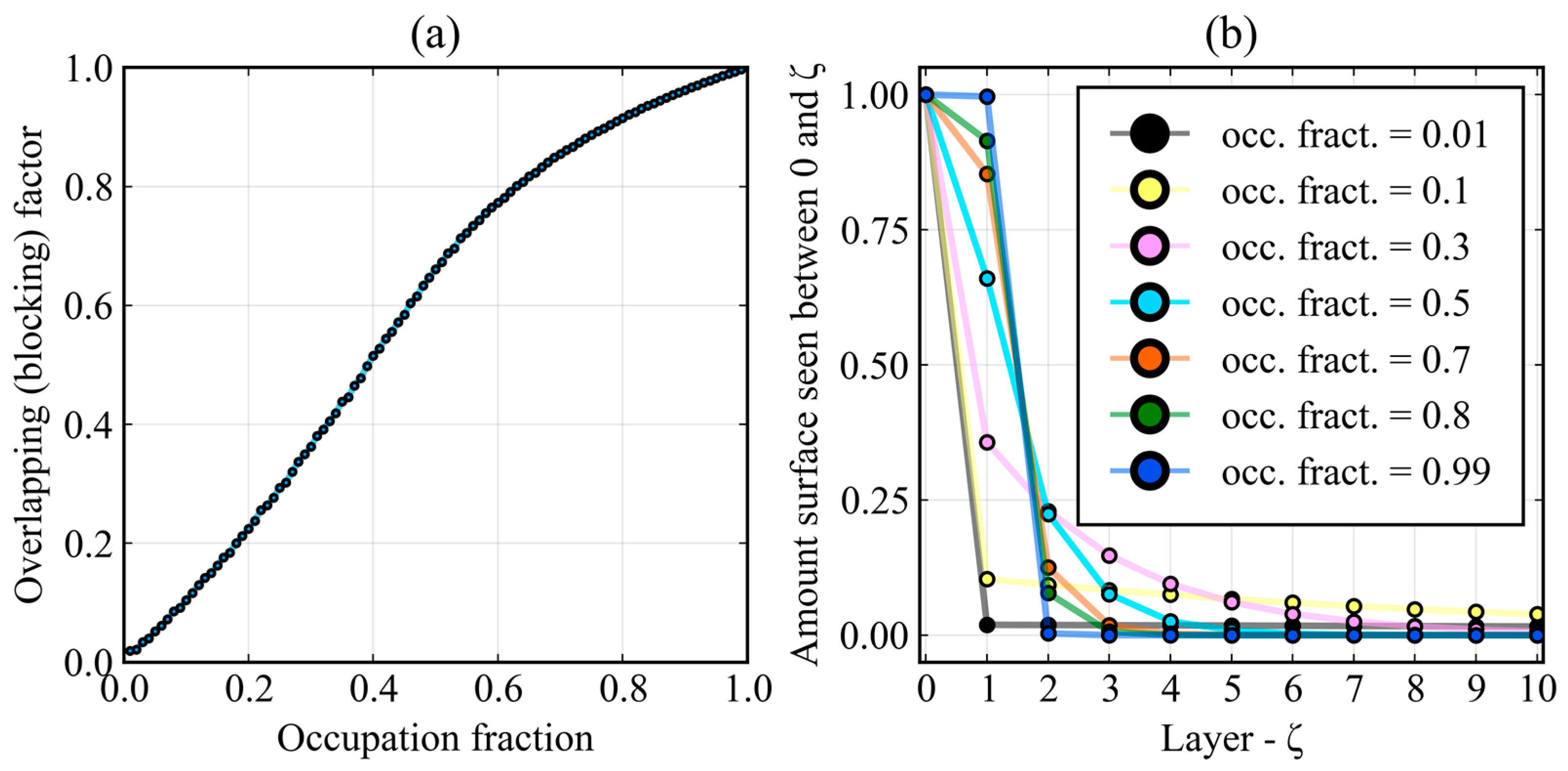
2.3.7. Radiation Modeling—Inside of the Scrap Bulk

As some of the thermal radiation between the scrap cells may penetrate though a single cell layer in $i$direction, due to its porosity, an approach to model this penetration behavior is necessary. Therefore, a scrap bulk thermal radiation simulation approach, to add additional radiation heat changes $\mathsf{\Delta }{Q}_{rad}$ to the evaluation of Equation (7), has been developed. This is somehow difficult, as changes in the modeling approach, according to the chosen cell size, must be made, because the radiation between the scrap pieces is not a continuous phenomenon. This is illustrated in Figure 7a, where you can see that if the cell size is chosen to large, radiation phenomena will probably be underestimated due to its highly nonlinear nature, and if it is chosen to be a lot smaller than the individual scrap pieces (Figure 7c), the individual heat transfer in each scrap piece may be underestimated, as well (especially if those have a high thermal conductivity and are not too elongated), as a single temperature (distribution) for each solid cell $i$ is being used. Therefore, choosing a cell size similar to the dimensions of an individual scrap piece seems reasonable (Figure 7b). This may not always be possible if the individual dimensions of the piece differ greatly from each other or the pieces itself are very large, so that a corresponding large cell size would lead to significant numerical errors.

For the calculation of radiation passing through the cells, some assumptions will be established. Furthermore, a simple model to calculate a cumulative blocking factor between the cell layer $i$ and its “seen” neighbor cells will be used. Therefore, it is assumed that there is an exposed surface in each cell, which contributes a certain amount of surface $A_{s,rad}$, which may be calculated using Equation (12) and represents the scrap surface, which can be “seen” by its adjacent cell at maximum. Within this equation, it must be considered that in theory, at maximum, some proportion less than half of the size of this surface area can be “seen” from each side of the cell, which leaves a specific unknown factor $c$ somewhere between zero and one, depending on the scrap geometry and distribution. This factor will cover for some side radiation losses, which cannot be represented in the 1D model, and further represent some kind of the only “self-seen amount” of the scrap parts in each cell. If the losses are ignored, which becomes increasingly true, the more cells are used (the smaller the cells become in respect to the shaft dimensions); this factor boils down to represent the not self-seen proportion of the surfaces. Furthermore, $c$ may also cover for the fact that through the structure of the radiation surfaces of the individual scrap pieces in the bulk, ${ϵ}_{eff}$ instead of the ideal $ϵ$ must be used, because of the cavity formation of the scrap pieces in the individual cells. Depending on the size and shape distribution of the individual scrap parts, $c$ will not be independent of the chosen cell size. Since there is no real knowledge of the quantity of this factor at the moment, a factor $c$ of 0.5 will be used.

$$A_{rad,layer i}=c\cdot 0.5\cdot SA:V_b\cdot V_{fs}$$

(12)

In this paper there, is no deep dive into the topic of how one could practically determine the factor $c$. For now, this factor should be looked at as a kind of optimization factor, which later could be adapted using real process data or adapted within sensitivity studies. If there are different scrap parts with different $c$ values inside the bulk, this model could in general be extended to a 2D or 3D model type, where influences of the composition could also be investigated.

Having the potentially radiation-blocking surface of each cell layer $i$, which is the same for each cell, a constant surface to volume area ratio and a constant cell size is used; there is a need for a model to estimate the penetration of thermal radiation through the individual cell layers. Therefore, a sub model, where the blocking surfaces of the individual scrap pieces in each cell over the cross-section area of the shaft are kind of unrolled into one dimension (see Figure 8a) has been developed. Furthermore, it is assumed that the scrap pieces are equally distributed over the cross-section area, but the distance between the individual pieces is allowed to vary randomly in between those equally distributed positions. If completely random positions of the individual pieces would be possible, dysfunctional scrap bulks would be part of consideration; for example, convectional heating would not work as intended. Due to the symmetry effects in such a system, this is similar to modeling two randomly positioned accumulated scrap piece areas against each other (Figure 8b). Then, the intersection areas (green lines in Figure 8) between the two layers for many (10,000 and more) randomly varied positions can be calculated.

Using this method, the overlapping factor $o_{fac}$ for each occupation fraction can be calculated, which is the fraction of the occupied shaft cross-section area by $A_{rad}$, shown in Figure 9a. Due to the fact that no completely random movement for the individual pieces has been set, the function deviates from a line with a slope of 1, where the average overlapping factor would be equal to the average occupation fraction.

Now, with this overlapping factor, the mean amount of surface, which can be seen between different cell layers $\zeta$, can be calculated using the Equation (13), in the following referred to as $b_{\zeta }$. Here, $b_{\zeta }$ is used as an array of values indexed according to $\zeta$. $\zeta$ is a relative coordinate system between a cell $i$ and its neighboring cell(s). This means that $\zeta =0$ refers to a cell itself and $\zeta =1$ refers to the exchange with the closest neighboring cell and so on.

$$\begin{array}{l}\zeta =0:1\\ \zeta =1:o_{fac}\\ \zeta >1:{\left(1-o_{fac}\right)}^{\zeta }\cdot o_{fac}\end{array}$$

(13)

The results are shown in Figure 9b. From this figure, it is seen that different occupation fractions may require a different amount of considered neighboring cells to accurately calculate the thermal radiation exchange between the individual cell layers. In this modeling approach, the exchange between an amount of $k$ neighboring layer cells is considered, where the amount of relative seen surfaces between $i$ and $i\pm k$ is greater than 0.1%. Of course, this is a gross simplification, which also worsens with increasing $\mathsf{\Delta }x$, because the calculated overlapping only directly correlates to radiation exchange for infinitely small distances, but it also is a fast and easy-to-calculate approach, which in the future also could be extended with additional optimization parameters to better fit reality.

Using the calculated $b_{\zeta }$ values, a modified version $b_{\zeta }^{*}$ were the entry for the layer index $\zeta =1$ of $b_{\zeta }$ is removed. Then, the restructured $b_{\zeta }^{*}$ must be indexed according to $\zeta =i-1$. The surface-to-surface radiation heat flow for the first $k$ cells of the bulk, going from the EAF side, can be calculated using the Equations (9)–(11). Using the aforementioned modification, the result according to $b_{\zeta }^{*}$ (see Equation (14)) can be evaluated. This procedure is physically not completely correct, as each cell layer $i$ of the first $k$ cells is simplified as being on the front layer of the bulk (Figure 6), including its corresponding temperature $T_i$, but it should be sufficiently accurate.

$$\begin{gathered} 0\le i<k:{\dot{Q}}_{i,rad,EAF}^{*}=b_i^{*}\cdot {\dot{Q}}_{i,rad,EAF}\left(T_i\right) \\ i\ge k:{\dot{Q}}_{i,rad,EAF}^{*}=0 \end{gathered}$$

(14)

To obtain the overall radiation heat transfer between a cell $i$ and its $k$ surrounding cells, an energy balance considering all cells within a certain range index range $k$ must be established, which again marks the range after which all outgoing radiation from a radiating cell should be absorbed. Therefore, Equation (15) has been derived. Here, the $c$ factor is considered within $A_{rad}$, which, according to the assumptions, is the same for each cell $i$. Furthermore, a modified equation for the heat transfer between two parallel equally sized surfaces, modified with the factor $b_{\zeta }$, which was introduced in the previous sections, is used with $\zeta =\left|i-\gamma \right|$.

$${\dot{Q}}_{i,rad,cross}=\sigma \cdot A_{rad}\cdot \left({\displaystyle \sum }_{\gamma =i-k}^{i-1}{b}_{\zeta }\cdot \frac{T_{\gamma }^4-T_i^4}{\frac{1}{{ϵ}_{s,i}}+\frac{1}{{ϵ}_{s,\gamma }}-1}+{\displaystyle \sum }_{\gamma =i+1}^{i+k}{b}_{\zeta }\cdot \frac{T_{\gamma }^4-T_i^4}{\frac{1}{{ϵ}_{s,i}}+\frac{1}{{ϵ}_{s,\gamma }}-1}\right)$$

(15)

Altogether, these equations should allow a decent modeling of the radiative transported heat inside the scrap bulk for higher temperature ranges. Unfortunately, one must estimate the mesh specific coefficient $c$ in a certain range.

3. Results

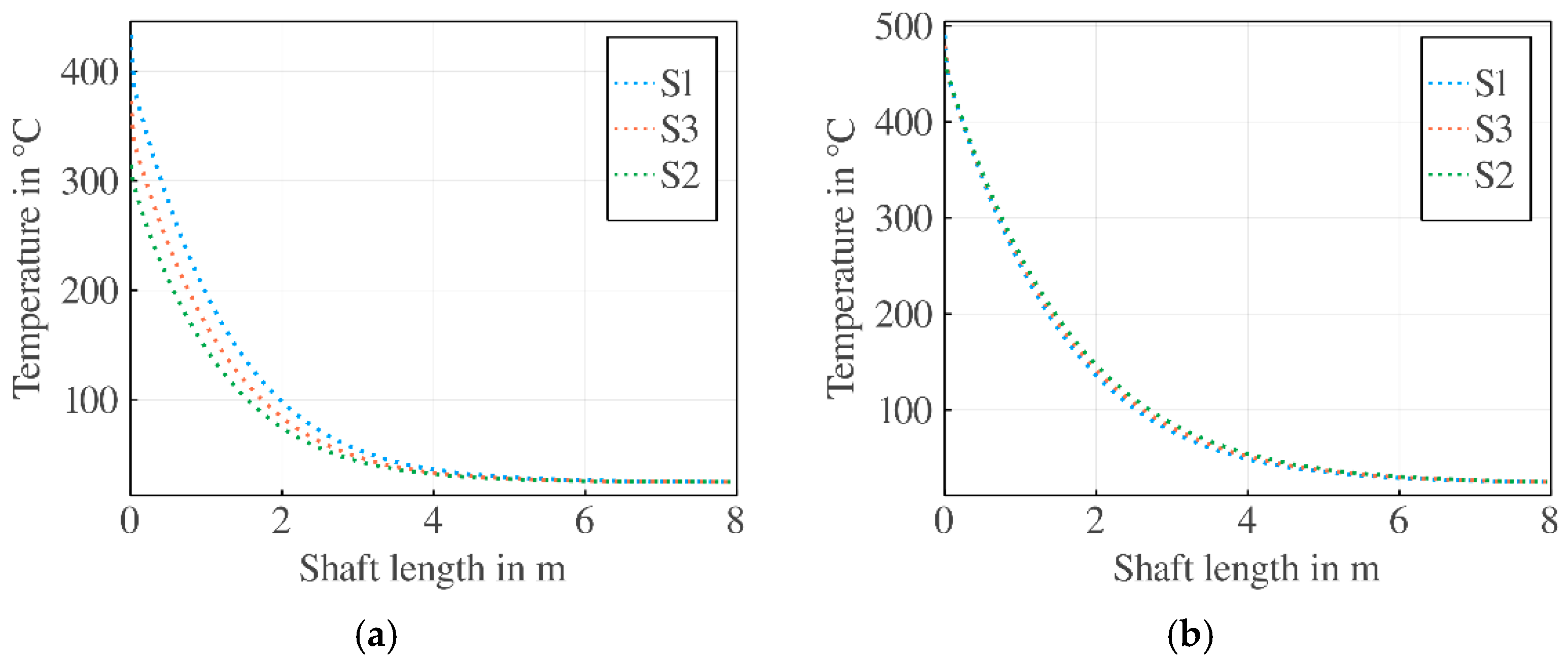
3.1. Model Sensitivity to Different Scrap Types

First, some results for three hypothetical scrap bulks consisting of different classes of scrap (see Table 1) are shown. In Figure 10, the predicted preheating temperature of the scrap (Figure 10a) and off-gas outlet temperature (Figure 10b) development over time can be seen. In Figure 10a, the resulting scrap temperature does not differ very much (deviation around 20 K), although the scrap characteristics defer in the range of usual scrap parts. Furthermore, as the outlet temperature of the off-gas is close to the charged scrap temperature (Figure 10b), nearly all energy is transferred from the off-gas to the scrap.

As it can be seen from Figure 10a, the scrap preheating temperature difference reduces over time of phase 1 under constant process conditions, which also applies to the spatial temperature distribution inside the bulk (see Figure 11a,b). From here on, the scrap type S3 is used for further investigations.

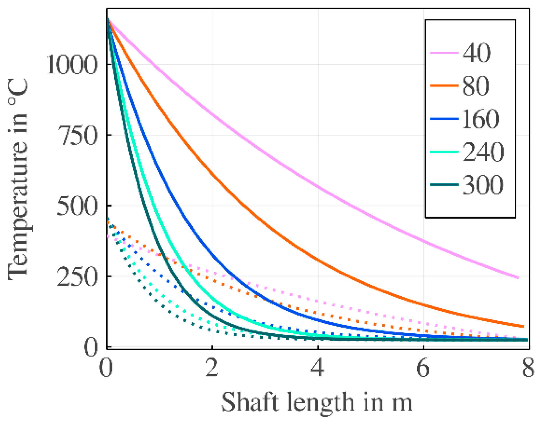
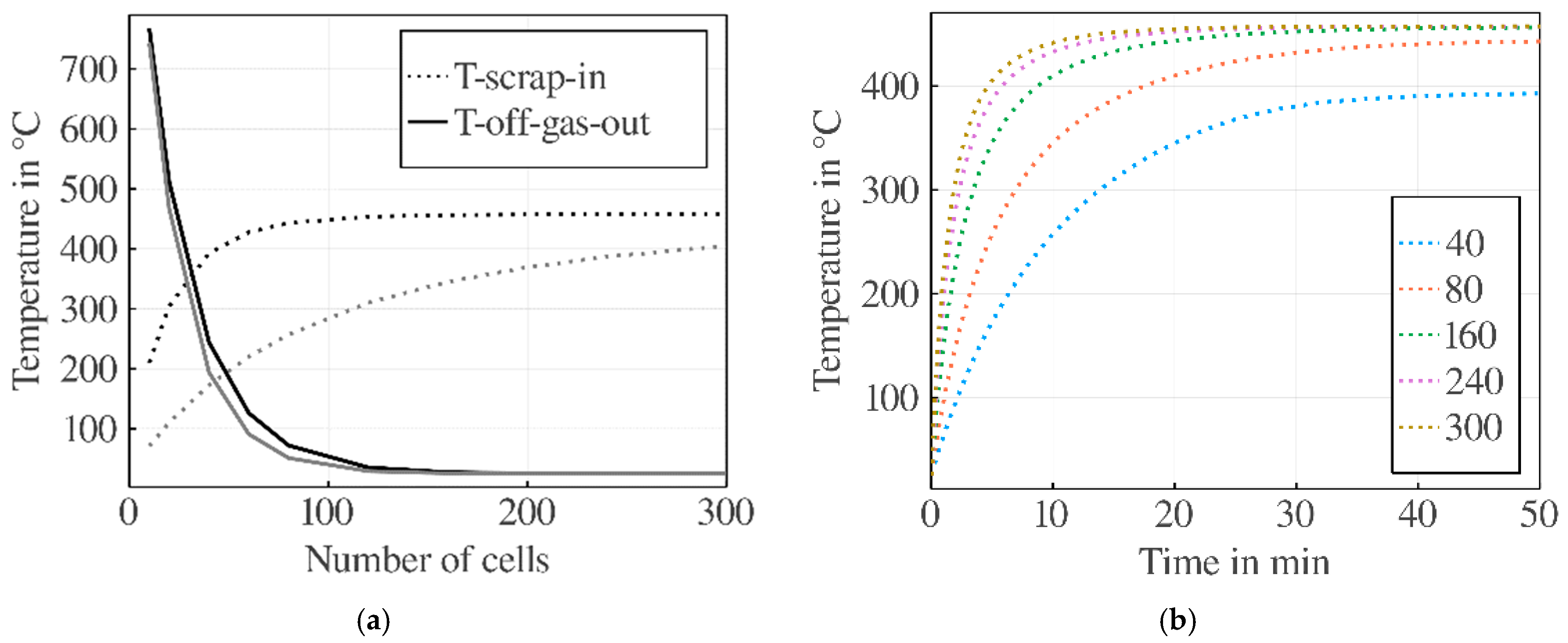
3.2. Mesh Size Implications on the Modeled Process

In Figure 12, the effect of the chosen mesh size on the temperature distribution over the shaft length is shown to be very pronounced. There are mainly two reasons for that. The first is the numerical convergence of the model regarding mesh size (convection, gas conduction) and the second is that the radiative heat transport is physically influenced by the mesh size, which basically is due to the geometry reduction to 1D. The numerical error of the convection modeling is amplified by the fact that there is no heat conduction model implemented over the length of the scrap for the scrap parts, therefore, the heat conduction in $x$ direction is theoretical infinite in each scrap cell and 0 between the scrap cells.

As the heat conduction in and between the scrap parts should not be the main transport mechanism, at least for the exemplary modeled process, the modeling error in this regard should be acceptable, if enough cells to significantly reduce the numerical error of the convective modeling are used. In Figure 13, the difference between the model using radiation modeling and no radiation modeling used in the model is shown at the end of the two different phases. As expected, the influence of thermal radiation, especially in the front of the bulk, are non-negligible in phase 2, while for phase 1, the influence especially in the main part of the bulk is very small.

Furthermore, looking at two main target properties, namely, the scrap preheating temperature and the off-gas temperature after the shaft, it can be seen from Figure 14a,b that these properties are converging for cell amount larger than ≈100 cells rather quickly when they approach a steady state condition.

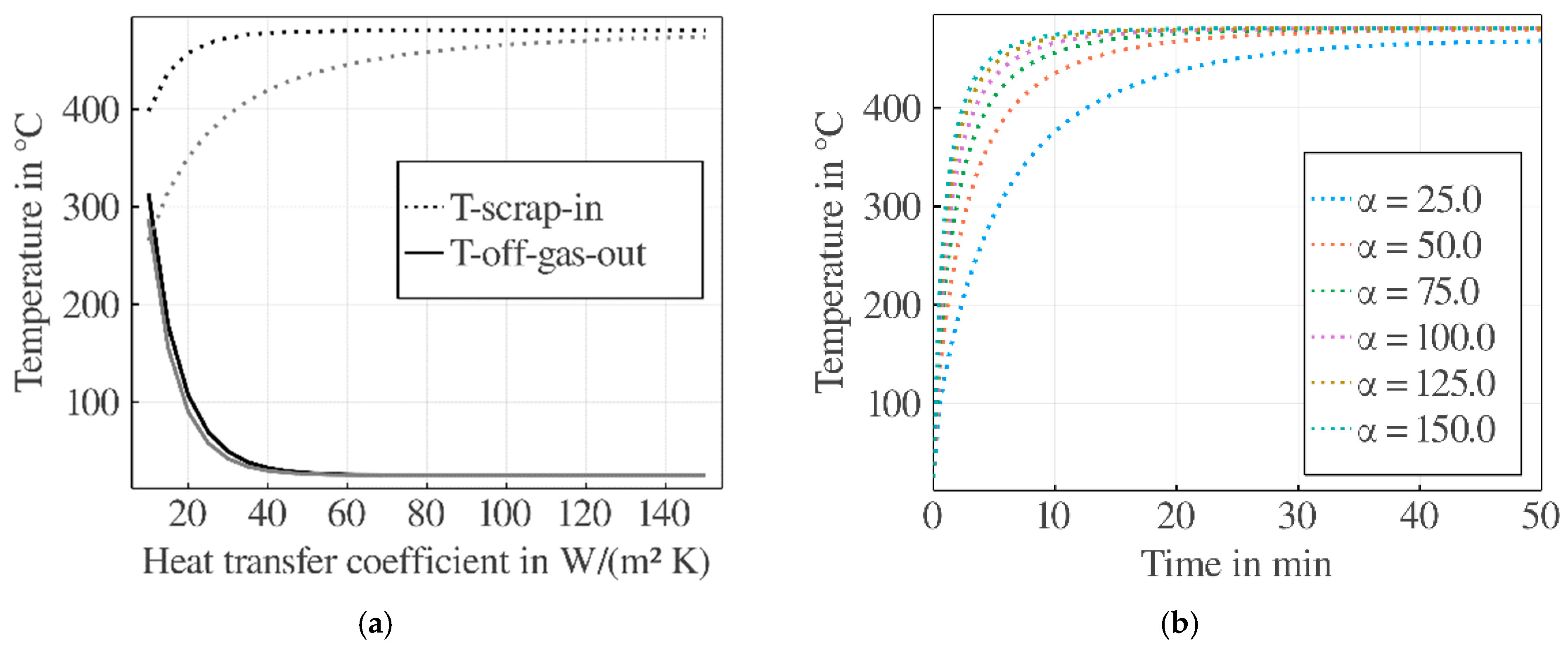
3.3. Influence of Convective Heat Transfer Assumptions

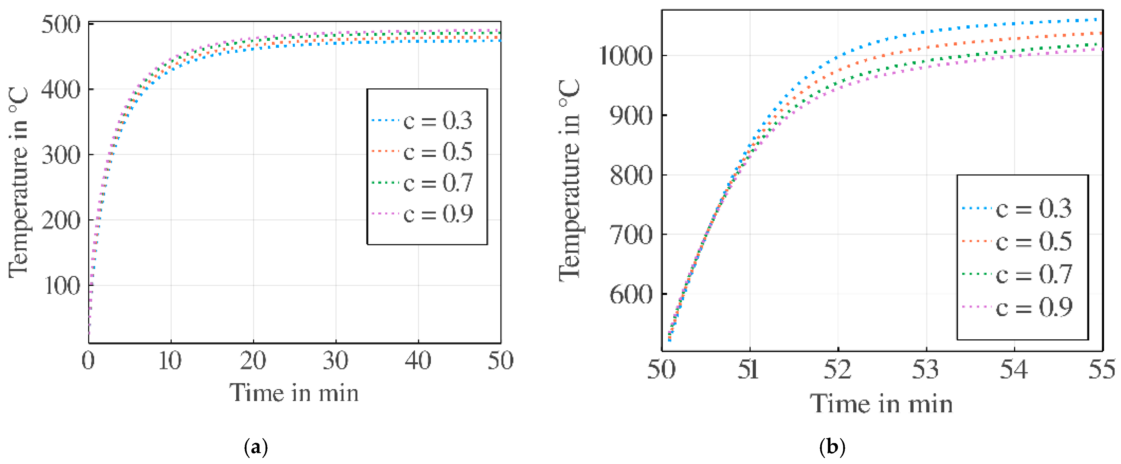
The influence of the used heat transfer coefficient is shown in Figure 15a,b. The simulation is very sensitive to the heat transfer coefficient in between 10 and 40 W/(m² K).

3.4. Influence of Factor $c$ on Modeled Radiative Heat Transfer

The importance of the factor $c$ does not seems to be of the most importance for the refining phase (phase 2) if the scrap temperatures inside the bulk are rising above 800 °C (Figure 16). During this phase (Figure 16b), deviations of around 50 °C can be observed between the predicted heating of the first scrap layer inside the scrap within varying $c$ between 0.3 and 0.9. As the flat-bath melting phase (Figure 16a) is clearly dominated by convective effects, differences are minor and around 10 °C.

Of course, there are other influences on the model, such as mass flow rates, material properties, etc., but these are rather well known. Therefore, they will not be described further.

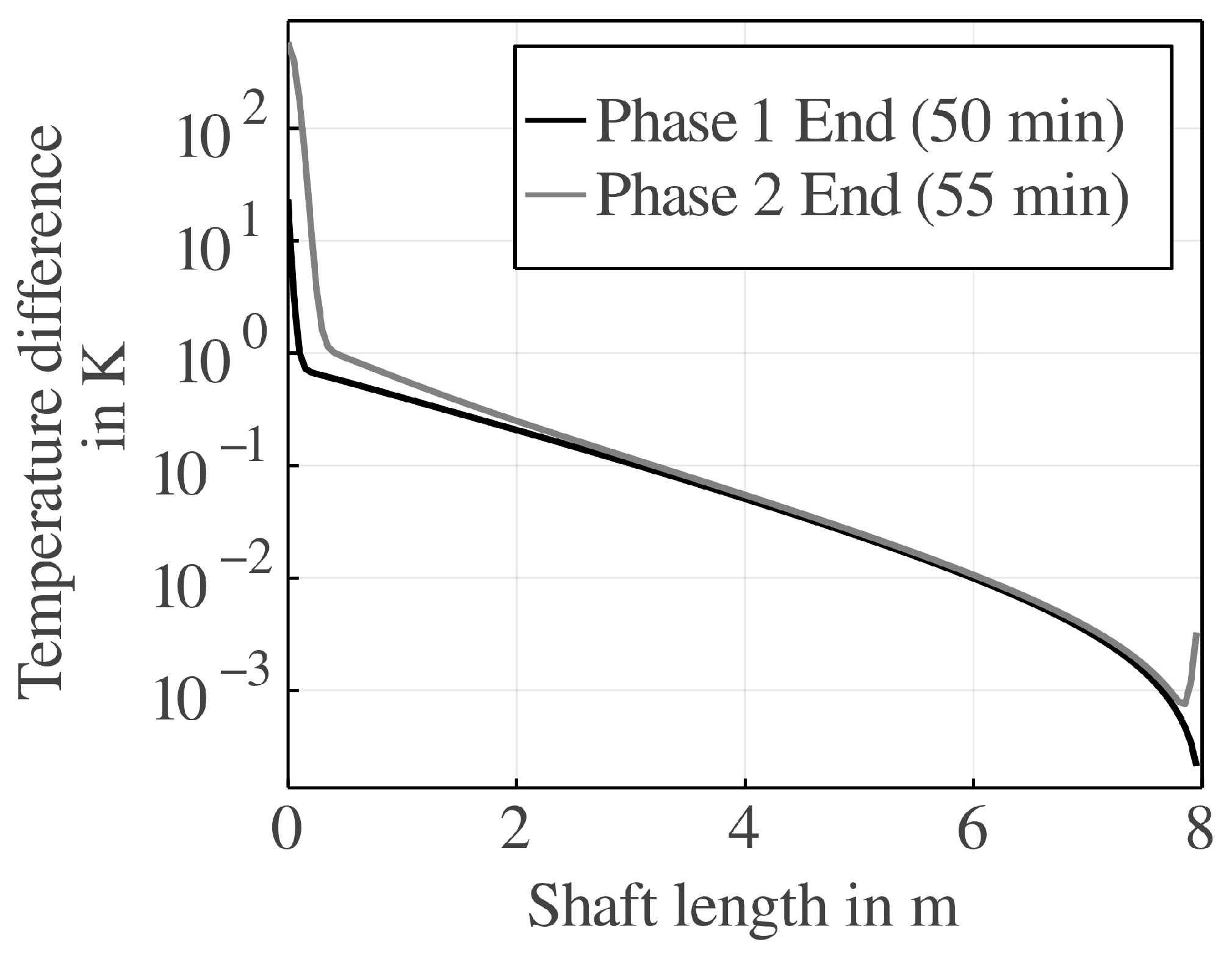
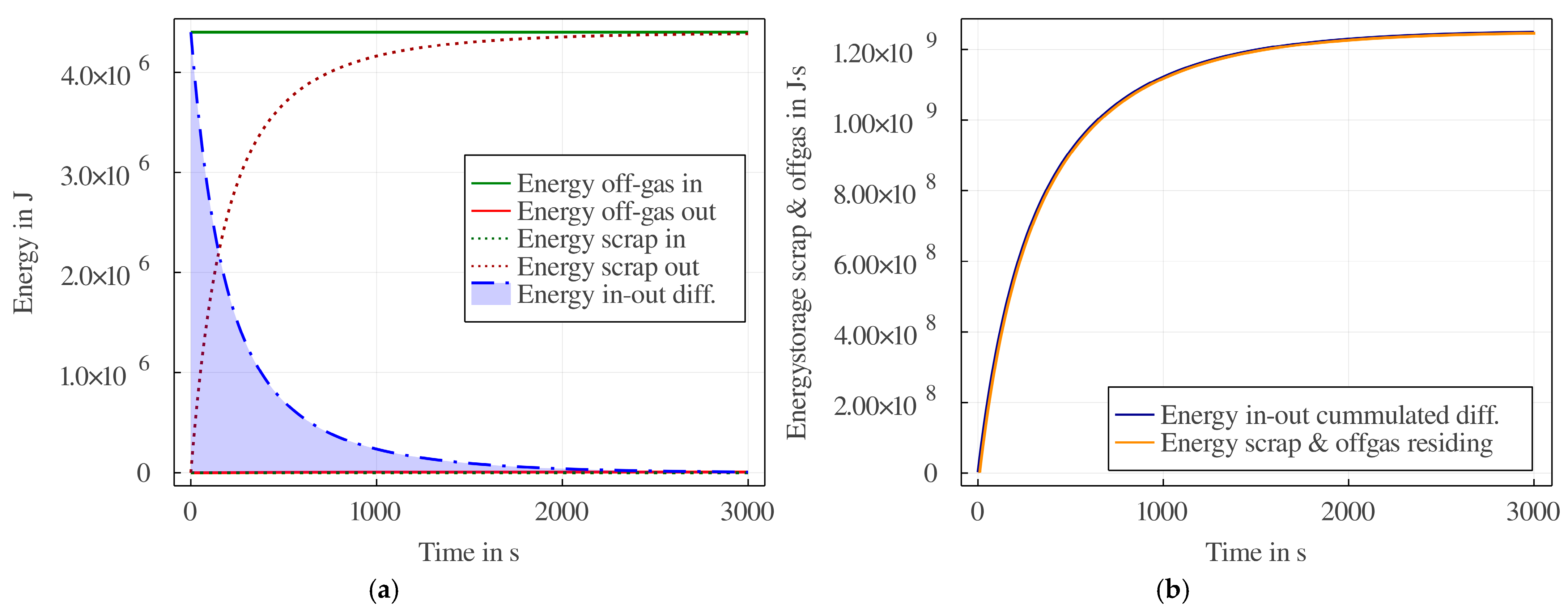
3.5. Verification of the Model’s Heat Balance

To give some exemplary verification of the correctness of the model’s implementation, energy in- and outputs to the shaft (scrap and off-gas), using the model without radiation transport model enabled, for the modeling of phase 1, are shown in Figure 17a.

In Figure 17b, the integral (blue area in Figure 17a) is shown as the blue curve. As the temperature distribution inside the bulk reaches a stationary state, the differences between the in- and output energies will approach zero; the energy difference accumulated up to this point in time must reside inside the scrap bulk. This is shown with the orange curve in Figure 17b, which depicts the stored energy inside the bulk (scrap and off-has) over the process time, which was calculated from the respective spatial temperature curves. There is a slight offset between the curves, which is due to the dynamics between changing the whole heating curve of the bulk and changing the preheating temperature of scrap in the first cell of the model. This indicates the mathematical correctness of the models regarding the overall energy balance.

4. Conclusions

The described modeling approach can deliver plausible results in short simulation times, usually much less than a minute for reasonable mesh sizes and simulated process times of ~60 min. Of course, the many simplifying assumptions lead to the fact that the shown results are not directly transferable to a real process. These simplifications were developed to clarify the impact of certain model aspects. It was shown that the scrap type for some variation of the different scrap classes will not have a very high impact on preheating temperatures (if the parts can be seen as thermally thin). Furthermore, we showed the importance of radiation modeling for rising temperatures in refining phase 2. It is interesting to note that some of the unknown model parameters, such as $c$, which have uncertainty and for a real process probably must be tuned against validation data, have much less influence than one could expect. Furthermore, it was shown that the current model is very sensitive (in the convection dominated phase) if low heat transfer coefficient values between 10 and 40 W/(m² K) are used. Nevertheless, these values are low for forced convection, but due to the relatively low velocities in the exemplary process between 0.5 m/s and 3 m/s (according to the assumed conditions and temperature ranges) it cannot be ruled out that these may occur in certain circumstances, as there are no general approximations of heat transfer coefficients in scrap bulks available in the literature now. Furthermore, due to the high temperature dependence of the gas’s density, the cooling will lead to a significant slowdown of the gas’s flow speed. Therefore, the derivation of heat transfer coefficients laws for different flow velocities through scrap bulks will be necessary to generate sufficiently accurate temperature estimates over the whole bulk.

From the results, it can be concluded that the shown modeling approach is very suitable, especially if radiation and convection phases can be separated. This can be justified by the fact that the convection model is strongly influenced by the number of cells used over the shaft length, while for the bulk radiation model, there is an additional physical implication of the chosen cell size. Separating the two is, therefore, a good way to avoid problems regarding the mesh. For mixed cases where both transmission mechanisms are important at the same time, an additional heat conduction model over the bulk length could help to reduce the numerical error for coarser meshes. Furthermore, the numerical error on a coarser mesh for the convective model could theoretically be mitigated by empirically or numerically determined compensation functions, so that an optimal grid size for the radiation modeling could still be chosen.

Certain cases such as inhomogeneous scrap movement of the bulk, mixed or variously layered scrap bulks may require the model to be extended to 2D or 3D, since those will be hard to account for in a 1D model. The capturing of other relevant aspects, such as varying off-gas properties (due to varying composition), the changing of flow rates (scrap and off-gas) over process time or the variation of heat transfer coefficient according to approximated gas velocities, is currently possible with the current model or rather does not require a lot of effort to implement. Nevertheless, such changes require validation data of existing processes.

5. Summary

To summarize, a fast and versatile scrap preheating model capable of estimating convective and radiation dominated heat transfer inside a scrap bulk, while also considering local heat conduction effects, has been developed. As shown, capturing the effects for the heating over the scrap part thickness is not very relevant for a broad range of different scrap types.

It was shown that in some areas, the model is not subject to strong deviations due to uncertainties in the model’s parameters; in many cases, it could therefore be used, for example, to estimate the approximate design of the required length of a scrap preheating shaft. Otherwise, under some circumstances, the model may be very reactive to some parameters. Therefore, it is recommended to start with investigating the model’s sensitivity to parameters as mesh size, used heat transfer coefficient and $c$. Furthermore, as there were no validation measurements performed for this model until now, practical decisions based on these results of our implementation should be carried out with the appropriate caution.

Additionally, there is still further work needed, especially regarding the areas of:

• Simplified modeling of conduction heat transfer between individual scrap parts, for applications where this becomes relevant;
• Validation and parameterization of the blocking modeling;
• Estimation strategies for the $c$ factor and the heat transfer coefficient ${\alpha }_{fs}$;
• Modeling of more complex scrap bulks with mixed materials;
• Finding suitable optimization factors to fit the model to various experimental cases.

Despite the several simplifications used in the model, the modeling approach itself is very extensible and, therefore, generally applicable to more complex cases, while still being as comprehensive as necessary to allow for real-time control and optimization purposes.

References

1. Coenen, L. Steel—The Surprising Recycling Champion. Available online: https://www.worldsteel.org/media-centre/blog/2018/blog-steel-surprising-recycling-champion.html (accessed on 20 February 2019).
2. Nardin, G.; Ciotti, G.; Dal Magro, F.; Meneghetti, A.; Simeoni, P. Waste Heat Recovery in the Steel Industry: Better Internal Use or External Integration?, XXIII Summer School “Francesco Turco”—Industrial Systems Engineering A New Model Proposal for Occupational Health and Safety Management in Small and Medium Enterprises; Summer School Francesco Turco: Palermo, Italy, 2018. [Google Scholar]
3. Toulouevski, Y.N.; Zinurov, I.Y. Electric Arc Furnace with Flat Bath—Achievements and Prospects; Springer: Berlin/Heidelberg, Germany, 2015; ISBN 978-3-319-15886-0. [Google Scholar]
4. Yang, Q.; Yang, L.; Shen, J.; Yang, Y.; Wang, M.; Liu, X.; Shen, X.; Li, C.; Xu, J.; Li, F.; et al. Polychlorinated Dibenzo-p-Dioxins and Dibenzofurans (PCDD/Fs) Emissions from Electric Arc Furnaces for Steelmaking. Emerg. Contam. 2020, 6, 330–336. [Google Scholar] [CrossRef]
5. Yang, L.; Jiang, T.; Li, G.; Guo, Y.; Chen, F. Present Situation and Prospect of EAF Gas Waste Heat Utilization Technology. High Temp. Mater. Process. 2018, 37, 357–363. [Google Scholar] [CrossRef]
6. Lehner, J.; Friedacher, A.; Gould, L.; Fingerhut, W. Low-Cost Solutions for the Removal of Dioxin from EAF Offgas. Rev. Met. Paris 2004, 101, 49–56. [Google Scholar] [CrossRef] [Green Version]
7. Dicion, A. Innovative Energy Conservation through Scrap Pre-Heating in an Electric Arc Furnace; ACEEE Summer Study on Energy Efficiency in Industry: 2013; p. 5. Available online: https://oaktrust.library.tamu.edu/handle/1969.1/149172?show=full (accessed on 1 July 2021).
8. SMS Group. Metallurgical Plant and Technology; Maenken Kommunikation GmbH: Köln, Germany, 2016; pp. 52–57. [Google Scholar]
9. CISDI Engineering Co. Ltd. (54). Steel Scrap Preheating-Type Electric arc Furnace and Method for Improving Heating Cold Area of Side Wall Charging Electric Arc Furnace. 2018. Available online: https://patents.google.com/patent/US10928136B2/en (accessed on 1 July 2021).
10. Manazzone, M.; Valoppi, A. ISMELT—Inteco Scrap MELting Technology Evolution. Available online: https://www.eases.rwth-aachen.de/dl/AOTK-2021/Manazzone_ISMELT%20%E2%80%93%20Inteco%20Scrap%20MELting%20Technology%20evolution.pdf (accessed on 18 June 2021).
11. Tang, G. Modeling of Steel Heating and Melting Processes in Industrial Steelmaking Furnaces. Ph.D. Thesis, Purdue University, West Lafayette, IN, USA, 2019. [Google Scholar]
12. Mandai, K. Modelling of Scrap Heating by Burners. Ph.D. Thesis, McMaster University, Hamilton, ON, Canada, 2010. [Google Scholar]
13. Arink, T.; Hassan, M.I. Metal Scrap Preheating Using Flue Gas Waste Heat. Energy Procedia 2017, 105, 4788–4795. [Google Scholar] [CrossRef]
14. Ioana, A.; Preda, A.; Be, L.; Moldovan, P.; Constantin, N. Improving Electric arc Furnace (eaf) Operation through Mathematical Modelling. UPB Sci. Bull. Ser. B 2016, 78, 185–194. [Google Scholar]
15. Schubert, C.; Eickhoff, M.; Pfeifer, H. Modelling of Continuous Scrap Preheating. In Proceedings of the 2019 STEELSIM Conference Proceedings, Toronto, ON, Canada, 13–15 August 2019; p. 8. [Google Scholar]
16. Zhang, L.; Oeters, F. Possibilities of Counter-Current Scrap Pre-Heating with Melting by Use of 100% Fossil Energy. Steel Res. 1999, 70, 296–308. [Google Scholar] [CrossRef]
17. Hay, T.; Visuri, V.-V.; Aula, M.; Echterhof, T. A Review of Mathematical Process Models for the Electric Arc Furnace Process. Steel Res. Int. 2020, 92, 2000395. [Google Scholar] [CrossRef]
18. Bezanson, J.; Edelman, A.; Karpinski, S.; Shah, V.B. Julia: A Fresh Approach to Numerical Computing. SIAM Rev. 2017, 59, 65–98. [Google Scholar] [CrossRef] [Green Version]
19. Bezanson, J.; Bolewski, J.; Chen, J. Fast Flexible Function Dispatch in Julia. arXiv 2018, arXiv:1808.03370v1. [Google Scholar]
20. StahlDat SX Professional: Register of European Steels. Available online: https://www.stahldaten.de/en/pub/home (accessed on 1 July 2021).
21. GERDAU Midlothian. Ferrous Raw Materials Manual—Part 3—Ferrous Raw Materialspecifications; GERDAU Midlothian Grade Specs: 2018. Available online: https://www2.gerdau.com/sites/gln_gerdau/files/downloadable_files/Midlothian%20Ferrous%20Raw%20Material%20Specifications.pdf (accessed on 1 July 2021).
22. Goodwin, D.G.; Speth, R.L.; Moffat, H.K.; Weber, B.W. Cantera: An Object-Oriented Software Toolkit for Chemical Kinetics, Thermodynamics, and Transport Processes. 2021. Available online: https://www.cantera.org (accessed on 30 May 2018).
23. Smith, G.P.; Golden, D.M.; Frenklach, M.; Moriarty, N.W.; Eiteneer, B.; Goldenberg, M.; Bowman, C.T.; Hanson, R.K.; Song, S.; Gardiner, W.C., Jr.; et al. GRI-Mech. Available online: http://www.me.berkeley.edu/gri_mech/ (accessed on 30 June 2020).
24. Rackauckas, C.; Nie, Q. DifferentialEquations.Jl—A Performant and Feature-Rich Ecosystem for Solving Differential Equations in Julia. J. Open Res. Softw. 2017, 5, 15. [Google Scholar] [CrossRef] [Green Version]
25. Alberti, M.; Weber, R.; Mancini, M. Gray Gas Emissivities for H2O-CO2-CO-N2 Mixtures. J. Quant. Spectrosc. Radiat. Transf. 2018, 219, 274–291. [Google Scholar] [CrossRef]
26. Hottel, H.C.; Sarofim, A.F. Radiative Transfer; McGraw-Hill: New York, NY, USA, 1967. [Google Scholar]
27. Howell, J.R.; Menguc, M.P.; Siegel, R. Thermal Radiation Heat Transfer; CRC Press: Boca Raton, FL, USA, 2015; ISBN 1-4987-5774-X. [Google Scholar]
28. Odenthal, H.-J.; Kemminger, A.; Krause, F.; Sankowski, L.; Uebber, N.; Vogl, N. Review on Modeling and Simulation of the Electric Arc Furnace (EAF). Steel Res. Int. 2018, 89, 1700098. [Google Scholar] [CrossRef]
29. Gruber, J.C.; Echterhof, T.; Pfeifer, H. Investigation on the Influence of the Arc Region on Heat and Mass Transport in an EAF Freeboard Using Numerical Modeling. Steel Res. Int. 2016, 87, 15–28. [Google Scholar] [CrossRef]
30. Coskun, G.; Yigit, C.; Buyukkaya, E. CFD Modelling of a Complete Electric Arc Furnace Energy Sources. Innovations 2016, 4, 22–24. [Google Scholar]
Figure 1. EAF off-gas preheating principle.
Metals 11 01280 g001
Figure 2. Thermophysical properties of steel 1.0035.
Metals 11 01280 g002
Figure 3. Thermophysical properties of the off-gas (70 vol.-% N2, 10 vol.-% CO2 and 20 vol.-% CO).
Metals 11 01280 g003
Figure 4. Illustration of first discretization step.
Metals 11 01280 g004
Figure 5. Modeling scheme of the 1D(–1D) model.
Metals 11 01280 g005
Figure 6. Discretized geometry used for view factor calculation.
Metals 11 01280 g006
Figure 7. Illustrative sketch of differently used cell sizes. (a) cell size >> scrap parts, (b) cell size scrap parts, (c) cell size << scrap parts.
Metals 11 01280 g007
Figure 8. Exemplary representations for the randomized overlap calculation (a) using eight individual scrap pieces, (b) using one.
Metals 11 01280 g008
Figure 9. Calculated occupation fractions (a) and amount of “seen” surface between a cell i and its neighboring cell ζ (b).
Metals 11 01280 g009
Figure 10. Simulated preheating temperature of scrap (a) and off-gas outlet temperature (b) over process time of phase 1 for the different characteristic scrap parts S1, S2 and S3 (see Table 1).
Metals 11 01280 g010
Figure 11. Simulated temperature distribution over the scrap bulk after (a) 5 and (b) 50 min.
Metals 11 01280 g011
Figure 12. Simulated scrap bulk (S3) temperature and off-gas temperature over the length of the shaft for different cell sizes after 50 min; dotted = scrap temperature, solid = off-gas temperature.
Metals 11 01280 g012
Figure 13. Comparison of resulting temperature differences radiation modeling in the bulk vs. no radiation modeling in the bulk at the ends of phase 1 and 2.
Metals 11 01280 g013
Figure 14. Scrap (S3) preheating and off-gas outlet temperature after 5 (gray lines) and 50 min (black lines) for different cell numbers (a); scrap (S3) preheating temperature development for cell numbers (b).
Metals 11 01280 g014
Figure 15. Scrap (S3) preheating and off-gas outlet temperature after 5 (gray lines) and 50 min (black lines) for different heat transfer coefficients a f s   ( = α ) (a); scrap (S3) preheating temperature development for different heat transfer coefficients a f s   ( = α )   (b).
Metals 11 01280 g015
Figure 16. Scrap (S3) preheating temperature development for different c values over the time of (a) phase 1 and (b) phase 2.
Metals 11 01280 g016
Figure 17. Energy in-, outputs and difference over time (a); cumulated energy difference and energy stored inside the bulk (scrap and off-gas) (b).
Metals 11 01280 g017