Biaxial Experiments and Numerical Analysis on Stress-State-Dependent Damage and Failure Behavior of the Anisotropic Aluminum Alloy EN AW-2017A

Abstract

Many experiments indicated the remarkable dependence of the strength and failure behavior of anisotropic ductile metals on the loading direction and on the stress state. These influences have to be taken into account in accurate material models and in the numerical simulation of complex loading processes predicting the safety and lifetime of aerospace structures. Therefore, the present paper discusses the effect of loading direction and stress state on the damage and failure behavior of the anisotropic aluminum alloy EN AW-2017A. Experiments and corresponding numerical analysis with the newly developed, biaxially loaded X0 specimen have been performed and the influence of different load ratios is examined. The formation of strain fields in critical parts of the X0 specimen is monitored by digital image correlation. Different failure modes are visualized by scanning electron microscopy of fracture surfaces. Stress states are predicted by finite element calculations and they are used to explain damage and fracture processes at the micro-level. The experimental–numerical analysis shows that the loading direction and the stress state remarkably affect the evolution of the width and orientation of localized strain fields as well as the formation of damage processes and fracture modes. As a consequence, characterization of anisotropic metals is highly recommended to be based on an enhanced experimental program with biaxial tests including different load ratios and loading directions.

1. Introduction

Several high-quality metals and alloys have been developed during the last few decades following requests from lightweight industry. For example, in the industrial aerospace sector, the main demands are increased safety and lifetime, improved cost efficiency and reduced energy consumption [1,2]. In particular, aluminum alloys have here a growing presence thanks to their quality and considerable lightness. Based on the optimization of material properties, it was possible to reduce the localization of irreversible deformations as well as damage and failure in critical parts of the structural elements of aircrafts. Damage at the micro-level can lead to ductile fracture on the macro-scale, which can be seen as the end of life of aerospace structures [3]. Prediction of the performance of manufactured parts is very important for aeronautical industries, where uncertainties may cause remarkable problems. As a consequence, detailed analysis of irreversible deformations as well as the damage and fracture behavior of these optimized metals and alloys is one of the main issues in engineering [4], allowing the proposition of accurate and practically applicable constitutive models [5,6]. These theoretical approaches must be based on experiments taking into account different loading directions and a wide range of stress states in order to be able to identify material parameters and to validate the constitutive theories for various engineering applications [7,8]. The special focus of the experimental–numerical analysis discussed in this paper is on the effect of different multi-axial stress states and of loading direction on damage and failure behavior in anisotropic metals.

Various experiments with different geometries of specimens have been presented in the literature to analyze the occurrence of inelastic deformations as well as damage and fracture processes at both the micro- and the macro-level. For example, unnotched and differently notched specimens have been uniaxially loaded to investigate the influence of stress state on inelastic strains and damage [9,10,11] or to examine fracture behavior in ductile metals [12,13,14,15]. On the other hand, special geometries of specimens undergoing shear deformation during uniaxial loading have been presented [16,17,18]. However, these experiments with uniaxially loaded specimens can only cover a small band of stress triaxialities, and this motivated an extended testing program with biaxially loaded cruciform specimens [19,20,21,22]. To achieved the required stress states, optimization of their geometries has been proposed [23,24,25]. In addition, further new geometries of cruciform specimens undergoing biaxial loading conditions have been developed to study the effect of different stress states on inelastic deformation as well as damage and fracture mechanisms in ductile metals [7,26,27].

Aluminum alloys undergo different forming processes, such as extrusion, rolling or deep drawing, to produce sheets for structural components in aircraft industries. In these forming techniques, large plastic strains cause anisotropies in the material due to internal changes in the crystallographic texture. Thus, in order to predict the mechanical behavior of ductile metal sheets in an accurate manner, induced anisotropies have to be taken into account in appropriate constitutive models. For example, Hill [28] proposed a quadratic function which can be seen as the anisotropic generalization of the von Mises criterion. However, in some applications, this yield function was not able to accurately predict both yield stresses and r values. Therefore, enhanced criteria based on non-quadratic functions have been used to model the anisotropic plastic behavior of metals [29,30,31]. Material parameters for these yield conditions are identified from different uniaxial and equi-biaxial tension tests. Alternatively, a quadratic yield criterion incorporating four hardening curves taken from uniaxial tension tests along rolling, diagonal and transverse directions as well as from equi-biaxial tests has been discussed [32]. In addition, new strategies for the calibration of anisotropic plasticity models based on the virtual fields method have been proposed [33,34].

During loading in various sheet metal forming operations, different stress states may cause different damage mechanisms on the micro-scale, and their accumulation can lead to various unexpected failure processes. Therefore, it is important to detect and to understand in detail these micro-mechanical mechanisms and their transition to the macro-level. Thus, a new set of experiments with the biaxially loaded X0 specimen, taking into account various load ratios and different loading directions in anisotropic ductile metals, is discussed in the present paper. Their influence on localized deformations as well as on damage and failure behavior is studied in detail using a combined experimental and numerical analysis. The investigated material is the aluminum alloy EN AW-2017A. It is a heat-treatable wrought alloy and is characterized by high tensile strength, excellent fatigue strength, very good corrosion resistance and machinabilty. It is used in various applications with high-strength structural components such as in machine construction, in military equipment, in aerospace industries as well as in transport and traffic applications. Material properties are characterized by uniaxial tension tests with dog-bone-shaped specimens taken from metal sheets in different directions. Results of biaxial tests with the X0 specimen are presented, where digital image correlation visualizes the formation of strain fields. In addition, scanning electron microscopy of the fractured surfaces reveals different damage and fracture mechanisms at the micro-level. Furthermore, the results of corresponding numerical simulations show stress states in critical parts of the specimens depending on loading directions and load ratios.

2. Material and Methods

2.1. Constitutive Model

The theoretical framework of the elastic–plastic deformation behavior of anisotropic ductile metals is mainly based on experimental investigations at the macro-level. In the proposed phenomenological model, the strain rate tensor

$${\dot{ϵ}}_{ij}={\dot{ϵ}}_{ij}^{el}+{\dot{ϵ}}_{ij}^{pl}$$

(1)

is additively decomposed into an elastic ${\dot{ϵ}}_{ij}^{el}$ and a plastic part ${\dot{ϵ}}_{ij}^{pl}$. The elastic behavior is assumed to be isotropic and is characterized by Hooke’s law, where the stress tensor can be expressed in the form

$${\sigma }_{ij}=2G{ϵ}_{ij}^{el}+\left(K-\frac{2}{3}G\right){ϵ}_{kk}^{el}{\delta }_{ij}$$

(2)

with the shear and the bulk modulus, G and K, of the investigated ductile metal, and ${\delta }_{ij}$ denotes the Kronecker delta (components of the unit tensor). In rolled sheets, the principal axes of anisotropy lie in the x direction of rolling (RD, $0^{\circ }$), in the y direction transversely in the plane of the sheet (TD, ${90}^{\circ }$) and in the z direction normal to this plane. It is assumed that the axes of anisotropy coincide with the principal axes of the stresses. In the present paper, anisotropic plastic behavior is governed by Hill’s [28] yield criterion

$$\begin{array}{c}\hfill f^{pl}\left({\sigma }_{ij}\right)=\sqrt{\frac{1}{2}\left[F{({\sigma }_y-{\sigma }_z)}^2+G{({\sigma }_z-{\sigma }_x)}^2+H{({\sigma }_x-{\sigma }_y)}^2+2L{\sigma }_{yz}^2+2M{\sigma }_{xz}^2+2N{\sigma }_{xy}^2\right]}-\overline{\sigma }=0\end{array}$$

(3)

where $F,G,H,L,M$ and N are material parameters which have to be identified by different uniaxial tests and $\overline{\sigma }$ represents the equivalent yield stress of a chosen reference test.

Furthermore, the evolution of plastic strains is predicted by an associated flow rule where the principal axes of the plastic strain rates coincide with those of the stresses. Thus, the rate of the plastic strain tensor is given by

$${\dot{ϵ}}_{ij}^{pl}=\dot{\overline{\lambda }}\frac{\partial f^{pl}}{\partial {\sigma }_{ij}}$$

(4)

where $\overline{\lambda }$ represents a non-negative factor characterizing the amount of plastic strain increments. Equation (4) takes into account plastic incompressibility (${\dot{ϵ}}_{ii}^{pl}=0$), which is usually observed in experiments with ductile metals [35].

In thin metal sheets, the identification of anisotropic material parameters is often restricted to experiments with specimens cut in its plane. Assuming plane stress conditions $({\sigma }_z={\sigma }_{xz}={\sigma }_{yz}=0)$, the yield criterion (3) reduces to

$$f_s^{pl}=\sqrt{\frac{1}{2}\left[(G+H){\sigma }_x^2-2H{\sigma }_x{\sigma }_y+(F+H){\sigma }_y^2+2N{\sigma }_{xy}^2\right]}-\overline{\sigma }=0$$

(5)

whereas the corresponding plastic strain rates (4) can be written in the form

$$\begin{array}{ccc}\hfill {\dot{ϵ}}_x^{pl}& =& \dot{\lambda }[(G+H){\sigma }_x-H{\sigma }_y]\hfill \\ \hfill {\dot{ϵ}}_y^{pl}& =& \dot{\lambda }[(F+H){\sigma }_y-H{\sigma }_x]\hfill \\ \hfill {\dot{ϵ}}_{xy}^{pl}& =& \dot{\lambda }N{\sigma }_{xy}.\hfill \end{array}$$

(6)

Based on the assumption of incompressible plastic deformation behavior, the plastic strain rate in the through-thickness direction is then given by

$${\dot{ϵ}}_z^{pl}=-({\dot{ϵ}}_x^{pl}+{\dot{ϵ}}_y^{pl})=-\dot{\lambda }(G{\sigma }_x+F{\sigma }_y).$$

(7)

For uniaxial tension tests with specimens cut at an angle $\alpha$ to the rolling direction of the thin sheet, the yield stresses in the principal directions of anisotropy are

$${\sigma }_x={\sigma }_{\alpha }{cos}^2\alpha ,{\sigma }_y={\sigma }_{\alpha }{sin}^2\alpha ,{\sigma }_{xy}={\sigma }_{\alpha }sin\alpha cos\alpha$$

(8)

where ${\sigma }_{\alpha }$ is the tensile yield stress in the $\alpha$ direction. With Equations (6) and (7), this leads to

$$\begin{array}{ccc}\hfill {\dot{ϵ}}_x^{pl}& =& \dot{\lambda }{\sigma }_{\alpha }[(G+H){cos}^2\alpha -H{sin}^2\alpha ]\hfill \\ \hfill {\dot{ϵ}}_y^{pl}& =& \dot{\lambda }{\sigma }_{\alpha }[(F+H){sin}^2\alpha -Hco{s}^2\alpha ]\hfill \\ \hfill {\dot{ϵ}}_z^{pl}& =& -\dot{\lambda }{\sigma }_{\alpha }(G{cos}^2\alpha -Fsi{n}^2\alpha )\hfill \\ \hfill {\dot{ϵ}}_{xy}^{pl}& =& \dot{\lambda }{\sigma }_{\alpha }Nsin\alpha cos\alpha .\hfill \end{array}$$

(9)

Computation of the ratios of measured plastic strain increments in tensile specimens cut in the x and y direction of the thin sheet as well as in its diagonal direction (DD, ${45}^{\circ }$) provide an alternative indirect method to determine the tensile and the shear yield stresses. Transformation of the plastic strain rates to the specimen’s orientation $\alpha$ and the corresponding transverse direction ($\alpha +{90}^{\circ }$) leads to

$$\begin{array}{ccc}\hfill {\dot{ϵ}}_{\alpha }^{pl}& =& {\dot{ϵ}}_x^{pl}{cos}^2\alpha +{\dot{ϵ}}_y^{pl}{sin}^2\alpha +2{\dot{ϵ}}_{xy}^{pl}sin\alpha cos\alpha \hfill \\ \hfill {\dot{ϵ}}_{\alpha +{90}^{\circ }}^{pl}& =& {\dot{ϵ}}_x^{pl}{sin}^2\alpha +{\dot{ϵ}}_y^{pl}{cos}^2\alpha -2{\dot{ϵ}}_{xy}^{pl}sin\alpha cos\alpha \hfill \end{array}$$

(10)

and with Equation (9), the requested plastic strain rate can be written in the form

$${\dot{ϵ}}_{\alpha +{90}^{\circ }}^{pl}=\dot{\lambda }{\sigma }_{\alpha }[-H+(G+F-2N+4H){sin}^2\alpha {cos}^2\alpha ].$$

(11)

The identification of the material parameters is based on the definition of the r values representing the ratios of the plastic strain increments in different directions ($\alpha +{90}^{\circ }$) and the through-thickness direction z, which can be written with Equation (7) in the form

$$r_{\alpha }=\frac{{\dot{ϵ}}_{\alpha +{90}^{\circ }}^{pl}}{{\dot{ϵ}}_z^{pl}}=\frac{-{\dot{ϵ}}_{\alpha +{90}^{\circ }}^{pl}}{{\dot{ϵ}}_x^{pl}+{\dot{ϵ}}_y^{pl}}.$$

(12)

Taking into account Equations (9) and (11), the r value is given by

$$r_{\alpha }=\frac{H+(2N-F-G-4H){sin}^2\alpha {cos}^2\alpha }{F{sin}^2\alpha +G{cos}^2\alpha }$$

(13)

allowing identification of the respective anisotropy parameters of the yield condition (Equation (5)).

2.2. Material and Parameters

The investigated material is the aluminum alloy EN AW-2017A (EN AW-AlCu4MgSi) supplied in the form of 4 mm thick sheets. The chemical decomposition is shown in

Table 1. Chemical composition of EN AW-2017A aluminum alloy (% weight).

Material	Cu	Fe	Mn	Mg	Si	Zn	Cr	Others	Al
EN AW-2017A	4.0	0.7	0.7	0.7	0.5	0.25	0.10	0.15	to balance

.

Specimens with different geometries are milled with high precision from these sheets. In some cases, notches are milled in the thickness direction. Based on photos of the micro-structures, these processes did not affect the material properties, remaining homogeneous over the investigated sections.

Identification of material parameters is based on tensile tests with specimens cut in different directions ($0^{\circ },{15}^{\circ },{30}^{\circ },{45}^{\circ },{60}^{\circ },{75}^{\circ },{90}^{\circ }$) from the aluminum alloy sheets. The tensile tests are performed in a uniaxial table test machine type inspekt Table 50-1 (produced by Hegewald & Peschke, Nossen, Germany) shown in Figure 1. Measurement of three-dimensional strain fields on the respective surfaces of the specimens is based on a special camera and lighting system, schematically shown in Figure 1a, using four cameras equipped with 75 mm lenses. Tensile tests were carried out three times for each direction, showing a very good correlation with only marginal differences. The geometry of the dog-bone-shaped specimen is shown in Figure 2. It is characterized by a long middle part, where nearly homogeneous stress and strain fields are expected to occur. This geometry has successfully been used in the lab of the authors during the last few years to identify elastic–plastic material parameters in ductile metals. During these tests, the geometry of the specimens remained homogeneous and necking occurred only during the last load steps. Thus, a uniaxial stress state was present, which was used to determine the respective true stresses.

Based on the measured strain fields, different r values can be determined using Equation (12), which are shown in Figure 3a. In addition, respective yield stresses ${\sigma }_{\alpha }$ are taken from true stress–true plastic strain curves of the different tensile tests with the specimens cut in the various directions $\alpha$ with respect to the rolling direction and are shown in Figure 3b. The reference yield stress $\overline{\sigma }$ is taken to be ${\sigma }_{0^{\circ }}$ for the specimen cut in the rolling direction (RD).

Furthermore, the numerical simulation of different biaxial tests is based on constitutive parameters identified by fitting the experimental equivalent stress–equivalent plastic strain curves of uniaxial tension tests in RD, DD and TD (Figure 4a). Isotropic elastic behavior is characterized by Young’s modulus $E=$ 74,000 MPa and Poisson’s ratio $\nu =0.3$. In addition, plastic hardening of the investigated aluminum alloy EN AW 2017 is adequately described by the Voce law [36] for the respective current yield stresses

$$c=c_o+R_o{ϵ}^{pl}+R_{\infty }\left(1-e^{-b{ϵ}^{pl}}\right)$$

(14)

with the initial yield stress $c_o$, the initial and final hardening moduli $R_o$ and $R_{\infty }$, the hardening exponent b as well as the equivalent plastic strain ${ϵ}^{pl}$.

For RD, DD and TD, the respective material parameters are shown in

Table 2. Plastic material parameters.

	${\mathit{c}}_{\mathit{o}}$ [MPa]	${\mathit{R}}_{\mathit{o}}$ [MPa]	${\mathit{R}}_{\mathbf{\infty }}$ [MPa]	b
RD	313	464	147	20
DD	308	474	127	28
TD	297	445	128	25

, leading to good agreement of the numerically predicted stress–plastic strain curves (Sim) with the experimental data (Exp) shown in Figure 4b. Deviations can only be seen at the end of the loading process (${ϵ}^{pl}=0.15$) after the onset of necking, leading to local three-dimensional stress states, as well as caused by damage processes that cannot be simulated by the elastic–plastic model.

The Lankford coefficients in RD, DD and TD (

Table 3. Lankford coefficients.

${\mathit{r}}_{\mathbf{0}}$	${\mathit{r}}_{\mathbf{45}}$	${\mathit{r}}_{\mathbf{90}}$
0.597	0.783	0.695

) are used to identify the anisotropy coefficients in the yield criterion (5). Using the results of the tensile test with the specimen cut in RD, the yield condition (5) with ${\sigma }_x=\overline{\sigma }$ and Equation (13) for $\alpha =0^{\circ }$ lead to

$$G=\frac{2}{1+r_{0^{\circ }}}$$

(15)

and

$$H=2-G.$$

(16)

In addition, with the results of the tensile test with the specimen cut in TD, the yield condition (5) leads to

$$F=\frac{2{\overline{\sigma }}^2}{{\sigma }_y^2}-H.$$

(17)

Alternatively, based on this experiment, the anisotropy parameter F can be computed using Equation (13) for $\alpha ={90}^{\circ }$:

$$F=\frac{H}{r_{{90}^{\circ }}}.$$

(18)

Furthermore, using the results of the tensile test with the specimen cut in DD, Equation (13) leads to

$$N=\left(r_{{45}^{\circ }}+\frac{1}{2}\right)(F+G).$$

(19)

Based on Equations (15), (16) and (18), this leads to the parameters G = 1.2523, H = 0.7477 and $F_{18}$ = 1.0758, which are able to accurately predict the experimental r values (Figure 3a, Fit 1, black curve), but leads to remarkable differences in the numerically predicted yield stresses with the experimental data (Figure 3b, Fit 1, black curve). Thus, the parameter F is alternatively determined with Equation (17), leading to $F_{17}$ = 1.4738. However, this leads to deviations in the numerically predicted r values (Figure 3a, Fit 2, blue curve) compared with the experimental ones, whereas the different yield stresses are well simulated. Therefore, the mean value of the respective parameters $F=\frac{1}{2}(F_{17}+F_{18})$ based on Equations (17) and (18) is computed, leading to acceptable numerical results for both the r values and the yield stresses (Figure 3, Fit 3, red curves). In addition, the parameter N is determined with Equation (19), and all anisotropy parameters are listed in

Table 4. Anisotropy parameters.

F	G	H	L	M	N
1.2747	1.2523	0.7477	3.0	3.0	3.2421

, which are used in the numerical simulations discussed in the next section.

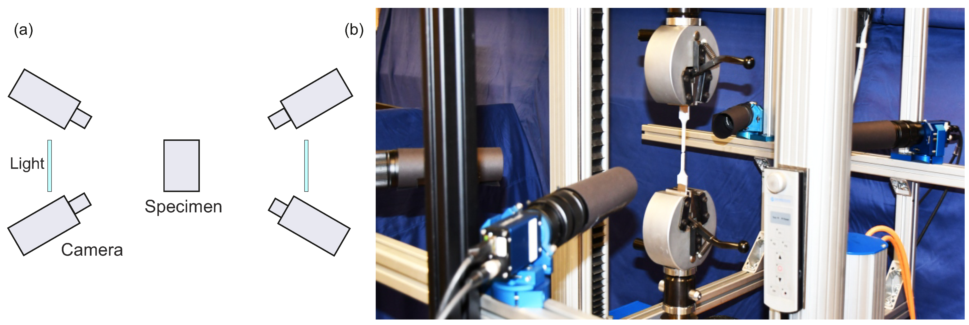
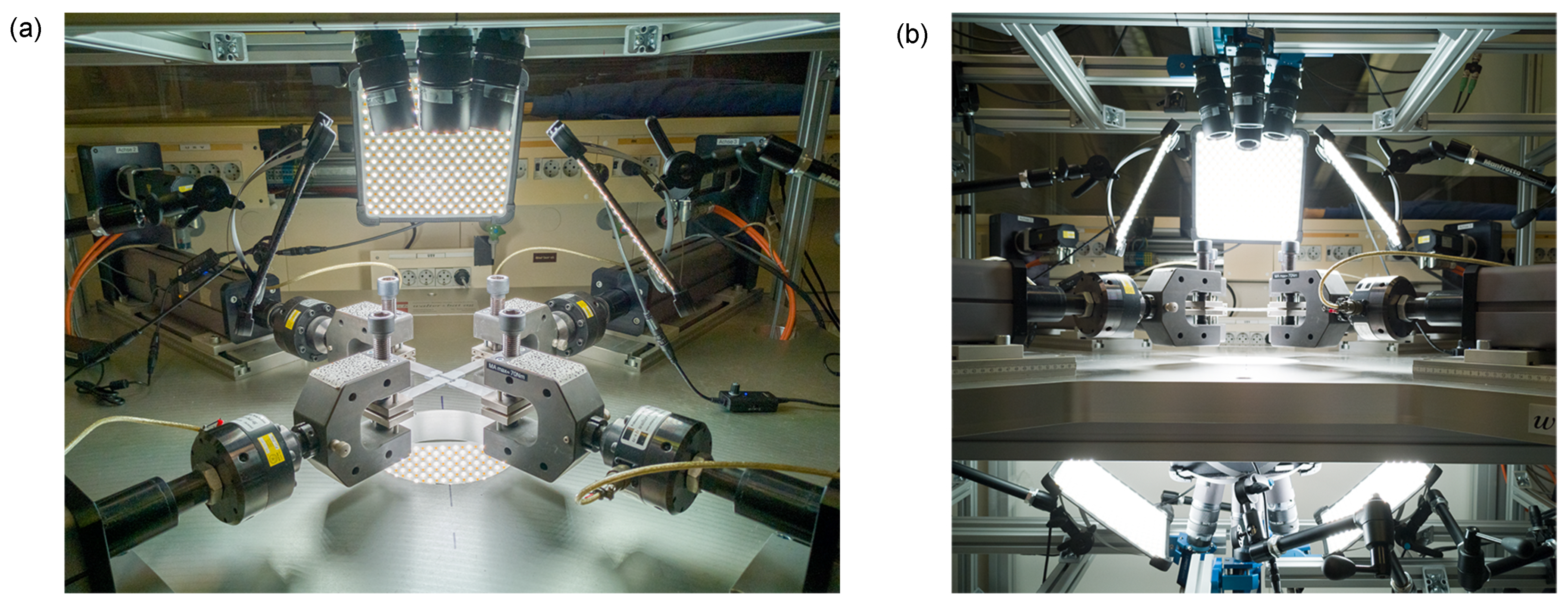
2.3. Experimental and Numerical Aspects

The biaxial experiments are performed in the test machine type LFM-BIAX 20 kN (produced by Walter & Bai, Löhningen, Switzerland). It contains four electro-mechanically driven actuators (Figure 5a), allowing individual tensile or compressive loading in two orthogonal axes. The experimental technique is described in detail in the References [7,37] and only the main aspects are briefly summarized in the present paper. In particular, the main machine displacement $u_{1.1}$ of cylinder $1.1$ in axis 1 (Figure 6f) is continuously increased by $0.004\mathrm{mm}/\mathrm{s}$. The same displacement is applied on the opposite side of the same axis on the cylinder $1.2$ as $u_{1.2}$. In the perpendicular axis 2, the cylinder $2.1$ is force-driven to guarantee constant load ratios during the experiment. This leads in this cylinder to the machine displacement $u_{2.1}$, and the same displacement is applied as $u_{2.2}$ on the cylinder $2.2$ on the opposite side of the axis 2. This technique has been shown to be remarkably stable and allows the performance of biaxial tests with cruciform specimens covering a wide range of requested stress states.

Before the experiments start, the specimens are clamped in the four heads of the actuators. Three-dimensional displacement fields in selected parts of the specimens are recorded during the tests by digital image correlation (DIC). Here, eight Allied Vision Manta G-609B/C cameras equipped with 75 mm lenses are used (Figure 5b). The corresponding lighting system (Figure 5) is installed in such a way that shadows and reflections are avoided within the notched parts of the specimens. During the experiments, the data sets of the digital image correlation system are stored with a frequency of 1.0 Hz. With this technique, the formation of strain fields on the boundaries of the specimens can be examined in detail, and strain localization phenomena as well as the onset of the evolution of macro-cracking can be revealed. The biaxial tests are carried out three times for each direction (RD, DD and TD) and each load ratio, showing a very good correlation with only marginal differences. Furthermore, the fracture surfaces of the failed specimens are analyzed by scanning electron microscopy (SEM) to visualize damage and fracture mechanisms at the micro-level.

For experimental examination of inelastic deformations and the stress-state-dependent failure behavior of ductile metals, new geometries of cruciform specimens have been proposed [7]. In the present paper, the X0 specimen (Figure 6a) is used to analyze the effect of anisotropic material characteristics on the multi-axial mechanical behavior of the investigated aluminum alloy sheets. The outer dimensions of the X0 specimen are 240 mm in both directions (b). In its center, notches in the thickness direction are milled (c), leading here to the localization of strain fields during loading. The length of the notched parts is 6 mm with a reduction in thickness up to 2 mm. The notch radii are 3 mm in plane (d) and 2 mm in the thickness (e) direction. The X0 specimen is simultaneously loaded in two perpendicular directions by $F_1$ and $F_2$ (f) with different proportional load paths. Displacements of the red points shown in Figure 6f, $u_{1.1}$ and $u_{1.2}$ in direction 1 and $u_{2.1}$ and $u_{2.2}$ in direction 2 are recorded by DIC during the experiments. They are used to determine the relative displacements $∆u_{\mathsf{ref}.1}=u_{1.1}-u_{1.2}$ and $∆u_{\mathsf{ref}.2}=u_{2.1}-u_{2.2}$ shown in the load–displacement curves.

On the numerical side, the finite element program ANSYS, enhanced by a user-defined material subroutine, is used to perform the numerical simulations of the experiments with the X0 specimens. The subroutine takes into account the plastic predictor–elastic corrector method to efficiently integrate the rate equations. A quarter of the X0 specimen is divided into 18,645 eight-node elements of type SOLID185 (Figure 7). Symmetry boundary conditions are used in the symmetry surfaces and the displacements are applied to the nodes at the end faces, whereas out-of-plane movements are prevented by zero displacements of the nodes in the symmetry plane in the out-of-plane direction. Refinement of the finite element mesh is taken into account in the notched parts of the X0 specimen to accurately predict the stress gradients and strain localization.

3. Results and Discussion

In the experimental program, different load ratios are considered. In particular, in the first case, the X0 specimen is uniaxially loaded by $F_1/F_2=1/0$, where direction 1 (Figure 6f) corresponds to the rolling direction (RD), the diagonal direction (DD) and the transverse direction (TD), respectively. In the second case, the X0 specimen is biaxially loaded by $F_1/F_2$ = 1/+1, leading to high tensile stresses in the notched region. Moreover, for this load ratio, loading direction 1 corresponds to RD, DD or TD. In the third case, the X0 specimen is biaxially loaded by $F_1/F_2$ = 1/−1, leading to shear behavior in the notches. Again, direction 1 corresponds to RD, DD or TD.

Experimentally obtained and numerically predicted load–displacement curves are shown in Figure 8. In particular, in the experiments with the load ratio $F_1/F_2=1/0$ (Figure 8a), an increase in load is observed up to $F_1=$ 9.2 kN for loading in RD, and the X0 specimen failed at the displacement $∆u_{\mathsf{ref}}=$ 1.08 mm. For loading in DD, the maximum load reaches $F_1=$ 8.7 kN whereas the final displacement at the onset of fracture is $∆u_{\mathsf{ref}}=$ 1.36 mm For loading in TD, the load increases up to $F_1=$ 9.0 kN and fails at the displacement $∆u_{\mathsf{ref}}=$ 1.21 mm. Thus, from the experiments with the X0 specimen loaded by $F_1/F_2=1/0$, it can be clearly seen that the loading direction with respect to the principal directions of anisotropy affects the maximum loads as well as the displacements at the onset of fracture. The loads differ by around $5\%$, where loading in RD leads to the highest load, whereas the smallest one is reached for loading in DD. The displacements at the onset of fracture differ by around $25\%$, where the largest displacement is measured for loading in DD and the smallest one for loading in RD. Therefore, these experimental results show that for loading in RD, the behavior is more brittle, whereas loading in DD leads to more ductile behavior.

This experimental behavior is reproduced by the numerical simulations based on the elastic–plastic constitutive model and on the parameters taken from the uniaxial tension tests discussed above. For loading in RD, the experimental and numerical load–displacement curves are nearly identical, whereas small differences can be seen for loading in DD and TD, but the main trends are well predicted. Thus, the Hill criterion (5) with the modified parameter identification method is able to adequately simulate the elastic–plastic deformation behavior of the investigated aluminum alloy.

In the experiments with the load ratio $F_1/F_2$ = 1/+1 (Figure 8b), similar load–displacement curves are obtained. For $F_1$ loading in RD, the maximum loads are $F_1=F_2=$ 9.2 kN and the X0 specimen failed at $∆u_{\mathsf{ref}.1}=$ 0.42 mm and $∆u_{\mathsf{ref}.2}=$ 0.45 mm, showing slightly non-symmetric behavior caused by inhomogeneities in the specimen’s geometry and inaccuracies in the experimental procedure. For $F_1$ loading in DD, the loads increase up to $F_1=F_2=$ 8.8 kN and the displacements at fracture are $∆u_{\mathsf{ref}.1}=∆u_{\mathsf{ref}.2}=$ 0.39 mm for both cases. For $F_1$ loading in TD, the loads reach $F_1=F_2=$ 8.9 kN and the specimen failed at $∆u_{\mathsf{ref}.1}=$ 0.40 mm and $∆u_{\mathsf{ref}.2}=$ 0.41 mm. Again, the $F_1$-loading direction with respect to the principal directions of anisotropy has an influence on load maxima and displacements at the onset of fracture, but in the case of the load ratio $F_1/F_2$ = 1/+1, the differences are only $5\%$ and $10\%$, respectively. Taking the ratio $F/∆u_{\mathsf{ref}}$ as an indicator for ductility or brittleness, no remarkable differences in ductility can be seen for the load ratio $F_1/F_2$ = 1/+1 in RD, DD and TD. However, compared to $F_1/F_2=1/0$, much smaller displacements are reached and, therefore, the behavior with respect to all loading directions is more brittle. In addition, numerically predicted load–displacement curves are also shown in Figure 8b, simulating very well the experimental behavior. Only a slight over-prediction of the final loads of less than $4\%$ can be seen but the main trends are nicely reproduced.

In the experiments with the load ratio $F_1/F_2$ = 1/−1 (Figure 8c), load–displacement curves for the positive and the negative load paths are obtained. In all cases, the orientations of $F_1$ loading (RD, DD and TD) of the load maxima are nearly identical, with $F_1=$ 5.1 kN and $F_2=$−5.3 kN, respectively. However, the displacements at the onset of fracture are different. For $F_1$ loading in RD, the displacements are $∆u_{\mathsf{ref}.1}=$ 1.16 mm and $∆u_{\mathsf{ref}.2}=$−1.40 mm, and for $F_1$ loading in DD, the final displacements are $∆u_{\mathsf{ref}.1}=$ 1.25 mm and $∆u_{\mathsf{ref}.2}=$−1.54 mm, whereas for $F_1$ loading in TD, $∆u_{\mathsf{ref}.1}=$ 1.07 mm and $∆u_{\mathsf{ref}.2}=$−1.32 mm have been measured. Thus, from these experiments with the X0 specimen loaded by $F_1/F_2$ = 1/−1, it can be clearly seen that the $F_1$ loading direction with respect to the principal directions of anisotropy affects the displacements at the onset of fracture, which differ by around $17\%$. They again show that the behavior for $F_1$ loading in DD is more ductile compared to the other loading directions. In addition, numerical simulations of these experiments have been performed. The numerical load–displacement curves are nearly identical for RD and TD whereas smaller loads are numerically predicted for DD. This trend agrees with the experimental observations and the numerical analysis, which only slightly over-predicts the experimentally measured loads with differences up to $10\%$. It should be noted that the numerical simulations are based on the proposed elastic–plastic model, whereas in the experiments, damage also takes place, leading to smaller loads.

During loading of the X0 specimen, strain fields in the notched regions are monitored by the digital image correlation (DIC) technique. At the end of the experiments, a sudden macro-crack is shown by DIC and strain fields are analyzed in the preceding photo shortly before fracture occurs. The first principal strain fields shortly before the onset of fracture are shown in Figure 9 for different load ratios and for different orientations with respect to the principal directions of anisotropy. In the left corner of each figure, the rolling direction is shown by the black lines. In particular, for the load ratio $F_1/F_2=1/0$ (Figure 9a) with loading in RD, small principal strain bands occur with a slightly diagonal orientation from top-left to bottom-right for the horizontal notches. During the loading process, the behavior in all four notches is nearly identical, and a few seconds before failure, a faster increase in strains is observed in the horizontal notches with maxima ${ϵ}_1=$ 0.35. Similar behavior is observed in the experiments with loading in DD, but higher strain maxima occur up to ${ϵ}_1=$ 0.40. For loading in TD, again, small principal strain bands are formed with later higher strain maxima up to ${ϵ}_1=$ 0.33 in the horizontal notches. In summary, for $F_1/F_2=1/0$, small principal strain bands occur with a slightly diagonal orientation and larger values for loading in DD, corresponding to the more ductile behavior also observed in the load–displacement curves (Figure 8a).

Figure 9b shows the experimental results for the load ratio $F_1/F_2$ = 1/+1. For $F_1$ loading in RD, more widespread bands of principal strains can be seen with maxima in an elliptical shape. The maxima are ${ϵ}_1=$ 0.22 in the horizontal notches. Very similar distribution of principal strains is measured for $F_1$ loading in DD, with slightly smaller values up to ${ϵ}_1=$ 0.20. Moreover, for $F_1$ loading in TD, again, these widespread bands can be seen, with strain maxima of ${ϵ}_1=$ 0.21. In summary, for the load ratio $F_1/F_2$ = 1/+1, for all loading directions, more widespread bands of high principal strains occur with horizontal/vertical orientation and the maxima form an ellipse. The distributions and the amounts of the final strains before fracture occurs only show small differences, which correspond to the very similar load–displacement curves in Figure 8b.

For the load ratio $F_1/F_2$ = 1/−1 (Figure 9c), the principal strains are localized in small strain bands with diagonal orientation from bottom-left to top-right for the horizontal notches. For $F_1$ loading in RD, the maxima are ${ϵ}_1=$ 0.41, whereas ${ϵ}_1=$ 0.43 is reached for DD. In the case of $F_1$ loading in TD, ${ϵ}_1=$ 0.40 occurs shortly before failure happens. These different values correspond to the different displacements at failure shown in the load–displacement curves (Figure 8c). In summary, the distribution, localization and orientation of principal strain bands are mainly caused by the load ratio, whereas the loading direction affects the maximum values.

Photos of the fractured specimens are shown in Figure 10. The fracture lines correspond to the localized bands of the maximum of the first principal strain (Figure 9), and remarkable inelastic deformations can also be seen in the non-failed notches, corresponding to high values of the principal strains. In particular, for the load ratio $F_1/F_2$ = 1/0 (Figure 10a), the fracture lines show a slightly diagonal orientation from top-left to bottom-right with a shear-dominated fracture mode. In the case of the load ratio $F_1/F_2$ = 1/+1 (Figure 10b), horizontal fracture lines can be seen with typical tensile-dominated fracture modes and cup-cone behavior. For the load ratio $F_1/F_2$ = 1/−1 (Figure 10c), the fracture lines are slightly diagonally oriented from bottom-left to top-right. The fracture modes are typical shear-dominated ones with smooth fracture surfaces. These experimental results clearly show that fracture lines on the macroscopic level are affected by the load ratios, whereas the influence of the loading direction (RD, DD or TD) is marginal.

Based on numerical simulations of the respective experiments, the stress states in the notched parts of the tested X0 specimens can be predicted. The stress parameters are evaluated after the last load step of the numerical analysis (see Figure 8). It should be noted that due to the experimental loading procedure with constant load ratios, the stress parameters remain nearly constant during the loading history in the plastic range. For example, the stress triaxialities $\eta$ (ratio of the mean stress and the equivalent stress) on the surface (S) and in the cross-section (C) of the notches are shown in Figure 11. For the load ratio $F_1/F_2=1/0$ (Figure 11a), the distribution of the stress triaxiality in the cross-section (C) is nearly homogeneous, with small gradients on the bottom and on the top. In the center of the notch, the stress triaxiality $\eta =$ 0.20 is numerically predicted, whereas on the bottom of the cross-section, $\eta =$ 0.35 is reached, and on its top, $\eta =$ 0.10 is reached. The influence of the loading direction on the stress triaxialities for this loading case is marginal. For the load ratio $F_1/F_2$ = 1/+1 (Figure 11b), higher gradients of the stress triaxiality can be seen in the cross-section (C) of the notched part of the X0 specimen. In the center of the notch, the stress triaxiality $\eta =$ 1.00 is reached, whereas on the boundaries of the cross-section (C) and on the surface (S), it is only $\eta =$ 0.40. The distribution is symmetric and, again, the effect of the $F_1$ loading direction is marginal. For the load ratio $F_1/F_2$ = 1/−1, the stress triaxialities are shown in Figure 11c. In this case, the distribution of the stress triaxialiy in the cross-section (C) of the notch is nearly homogeneous, with only small gradients on the bottom and on the top. In the center of the notch, $\eta =$ 0.00 is numerically predicted, whereas in small regions on the bottom, $\eta =$ 0.33 and on the top $\eta =$ 0.11 are reached. On the surface (S) of the notch, the stress triaxiality is also nearly homogeneous, with $\eta =$ 0.00. Again, the influence of the $F_1$ loading direction is marginal. These numerical results have clearly shown that the amount and distribution of the stress triaxialities in the notches of the X0 specimen remarkably depend on the load ratio, whereas they are only marginally influenced by the loading direction (RD, DD and TD).

After the tests, the fracture surfaces have been analyzed by scanning electron microscopy (SEM) and the respective pictures of the center of the fracture surface are shown in Figure 12. In particular, for the load ratio $F_1/F_2=1/0$ (Figure 12a) after loading in RD, many voids and some shear mechanisms can be seen, leading to sheared dimples. For loading in DD, only some small voids occur but more micro-shear-cracks and sheared voids are visible. For loading in TD, voids and micro-shear-cracks can be seen, with small sheared dimples. However, the stress triaxiality for all loading directions was nearly identical, with $\eta =$ 0.20 in the center of the notch (Figure 11a), and for isotropic materials, the mixed failure mode with the simultaneous growth of voids and the formation of micro-shear cracks is expected to occur for this moderate stress triaxiality [12,37]. In the case of the investigated anisotropic material, the failure mode also depends on the loading direction, with more superimposed void growth for loading in RD and more pronounced shear mechanisms for loading in DD.

On the other hand, for the load ratio $F_1/F_2$ = 1/+1 (Figure 12b), $F_1$ loading in RD leads to remarkable void growth, with large pores and clear dimples. For $F_1$ loading in DD, the voids are smaller but also lead to dimples, which are smaller compared to those after loading in RD. For $F_1$ loading in TD, again, large pores and clear dimples similar to those observed after loading in RD can be seen. With the high stress triaxiality, $\eta =$ 1.00 is numerically predicted for this load ratio in the center of the notch (Figure 11b); for isotropic materials, remarkable void growth is expected to occur [25]. This also happens for the examined anisotropic material but the $F_1$ loading direction has an influence on the size of the voids. They are larger for loading in RD and TD, whereas smaller pores can be seen after loading in DD.

For the load ratio $F_1/F_2$ = 1/−1, the SEM pictures are shown in Figure 12c. For $F_1$ loading in RD, some small voids are formed, which are sheared and superimposed by micro-shear cracks. For $F_1$ loading in DD, nearly no voids occur and failure is caused by the accumulation of micro-shear cracks, leading to a very smooth and flat failure surface. For $F_1$ loading in TD, again, some voids can be seen, which are sheared and superimposed by micro-shear cracks. Compared to loading in RD, here, more and slightly larger voids are visible. Based on the results for isotropic materials [25,27], namely the the numerically predicted stress triaxiality $\eta =$ 0.00 in the center of the notch (Figure 11c), micro-shear-crack behavior without the formation of voids is expected to occur. However, in the case of the investigated anisotropic material, the failure mode also depends on the $F_1$-loading direction. The expected mode only occurs for loading in DD, whereas for loading in RD and TD, the additional formation of small voids has been revealed by SEM. In summary, although no dependence on the loading direction of the stress triaxiality (Figure 11) and of the macroscopic fracture lines (Figure 10) has been detected by the experimental and numerical analysis, the SEM pictures have shown the effect of the loading direction on the damage and fracture mechanisms on the micro-scale. For all load ratios, there is greater formation and growth of voids during loading in RD and TD, whereas smaller or no voids occur during loading in DD. Thus, the SEM analysis clearly shows that for high stress triaxialities, the influence of the loading direction on damage and failure mechanisms at the micro-level is small; in all cases, predominant formation and growth of voids is observed, and only the size of the voids is larger for loading in RD and TD and smaller for loading in DD. However, for moderate and zero stress triaxialities, a remarkable effect of the loading direction on these microscopic processes has been detected. For loading in RD and TD, mixed failure mechanisms with simultaneous growth of voids and formation of micro-shear cracks occurred, and their proportion depends on the stress triaxiality (decrease in stress triaxiality leads to more micro-shear cracks). For loading in DD, at the same level of stress triaxiality, the formation of micro-shear cracks is more predominant and the growth of voids is lower. This loading-direction-dependent behavior can also be seen in the load–displacement curves (Figure 8). For high stress triaxialities (load ratio $F_1/F_2$ = 1/+1, Figure 8b), the differences in loads and displacements at the onset of fracture are small and the behavior was brittle, corresponding to the predominant void growth. However, for moderate ($F_1/F_2=1/0$, Figure 8a) and zero ($F_1/F_2$ = 1/−1, Figure 8c) stress triaxialities, loading in DD leads to larger displacements, indicating more ductile behavior corresponding to shear-dominated behavior at the micro-level.

4. Conclusions

In this paper, the influence of the loading direction and the stress state on the damage and fracture behavior of the anisotropic aluminum alloy EN AW-2017A has been investigated in detail. Various experiments and numerical simulations with the biaxially loaded X0 specimen have been performed with a focus on different load ratios and loading directions. The main conclusions are:

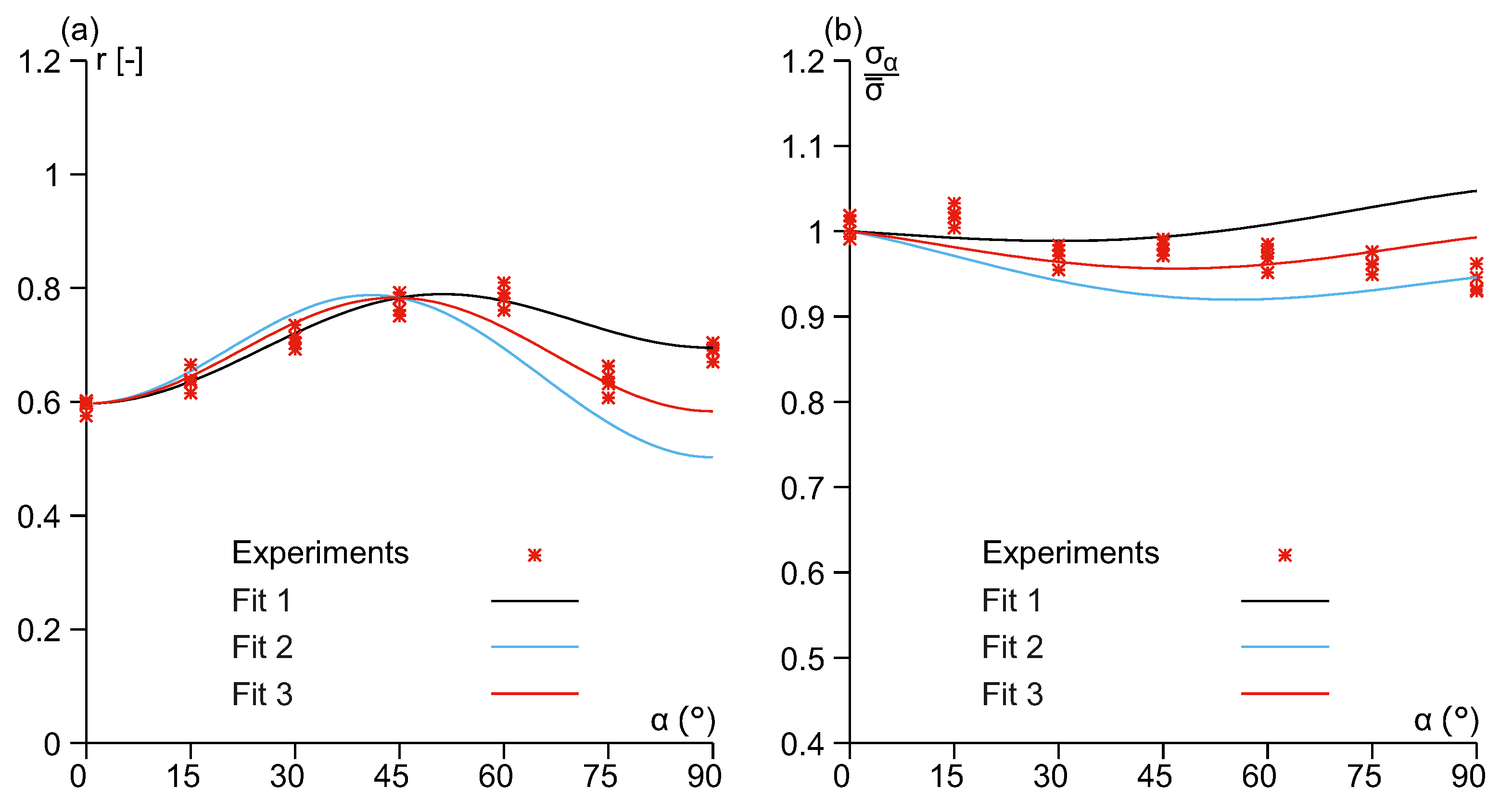
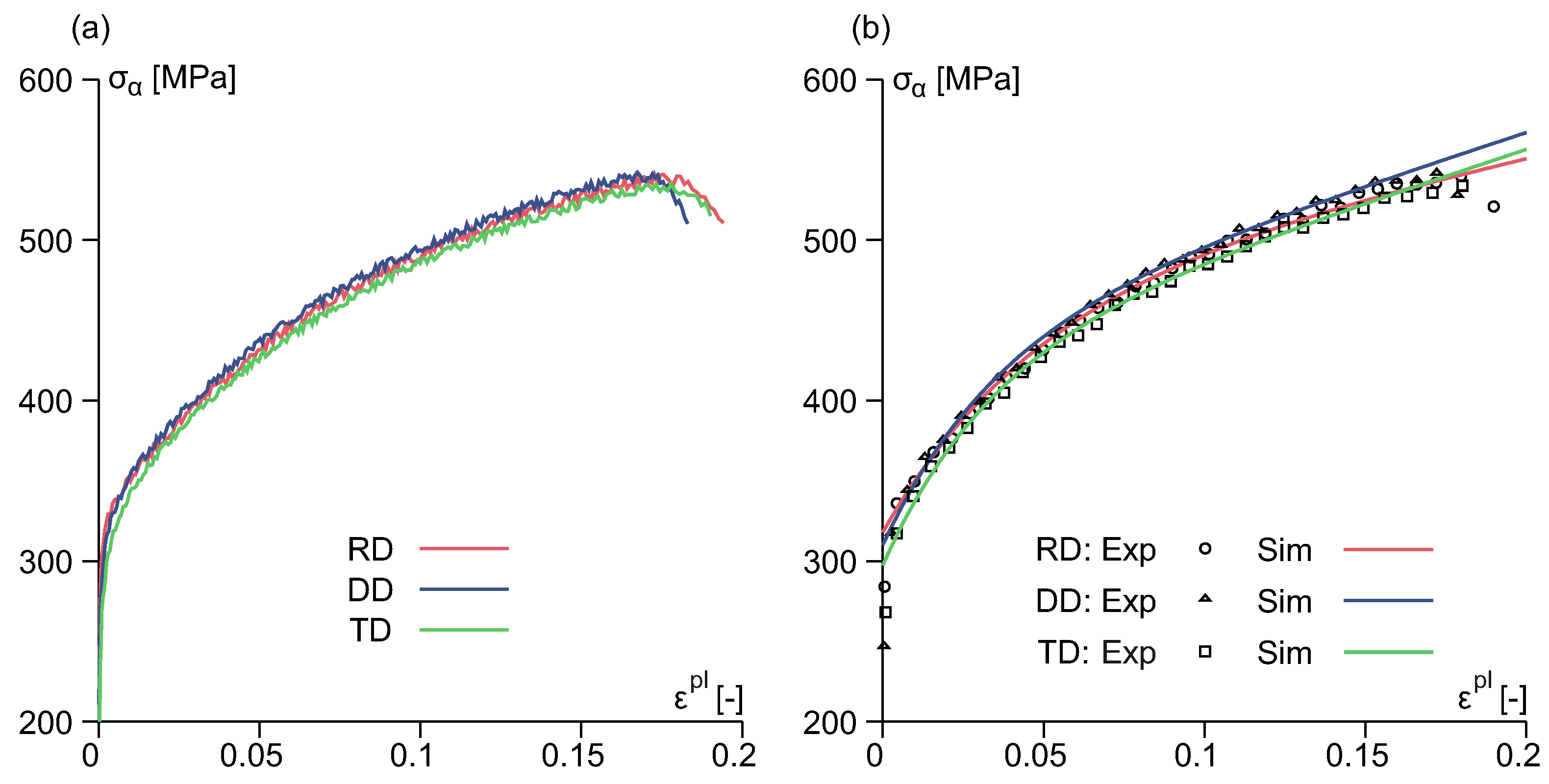
• The anisotropy parameters in Hill’s yield criterion are determined by a combined method using the yield criterion and the r values. This leads to accurate prediction of both the yield stresses and the r values measured in tension tests with different loading directions.
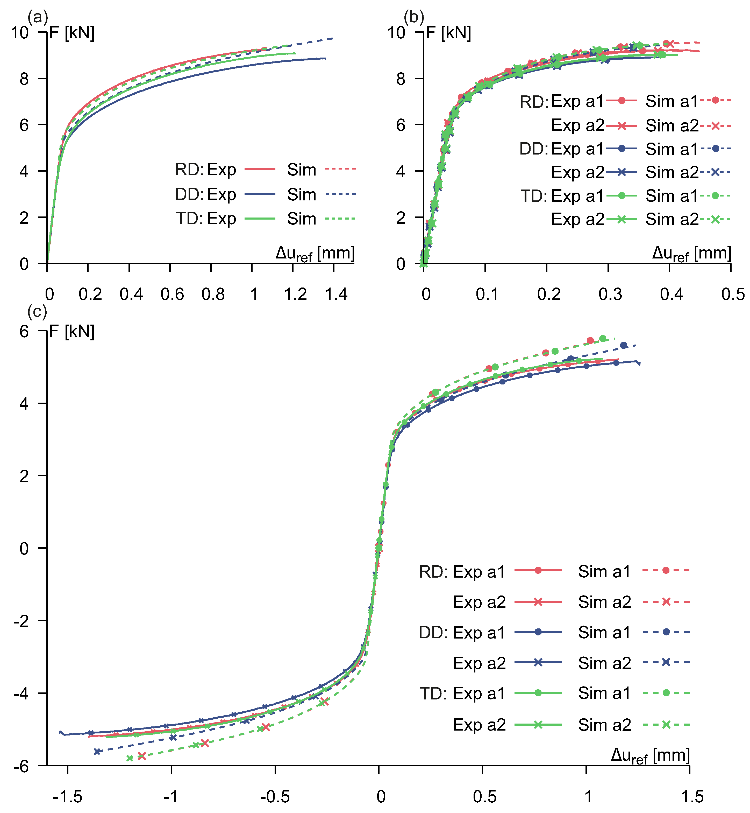
• The loading direction affects the load–displacement behavior in biaxial experiments. For load ratios leading to moderate or zero stress triaxialities, larger displacements occur for loading in DD and smaller ones for loading in RD. Thus, for these stress states, the deformation behavior for loading in DD is more ductile.
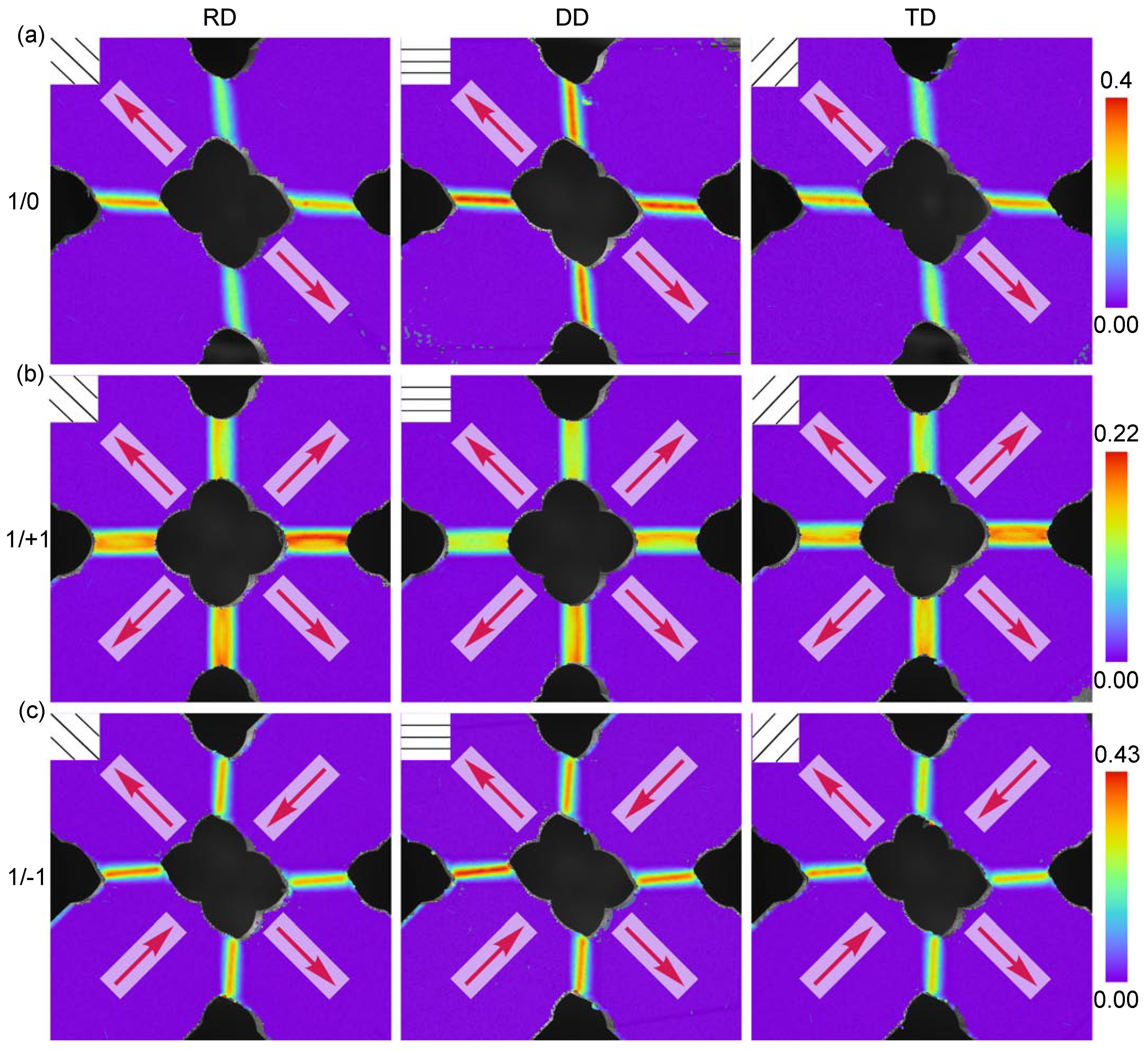
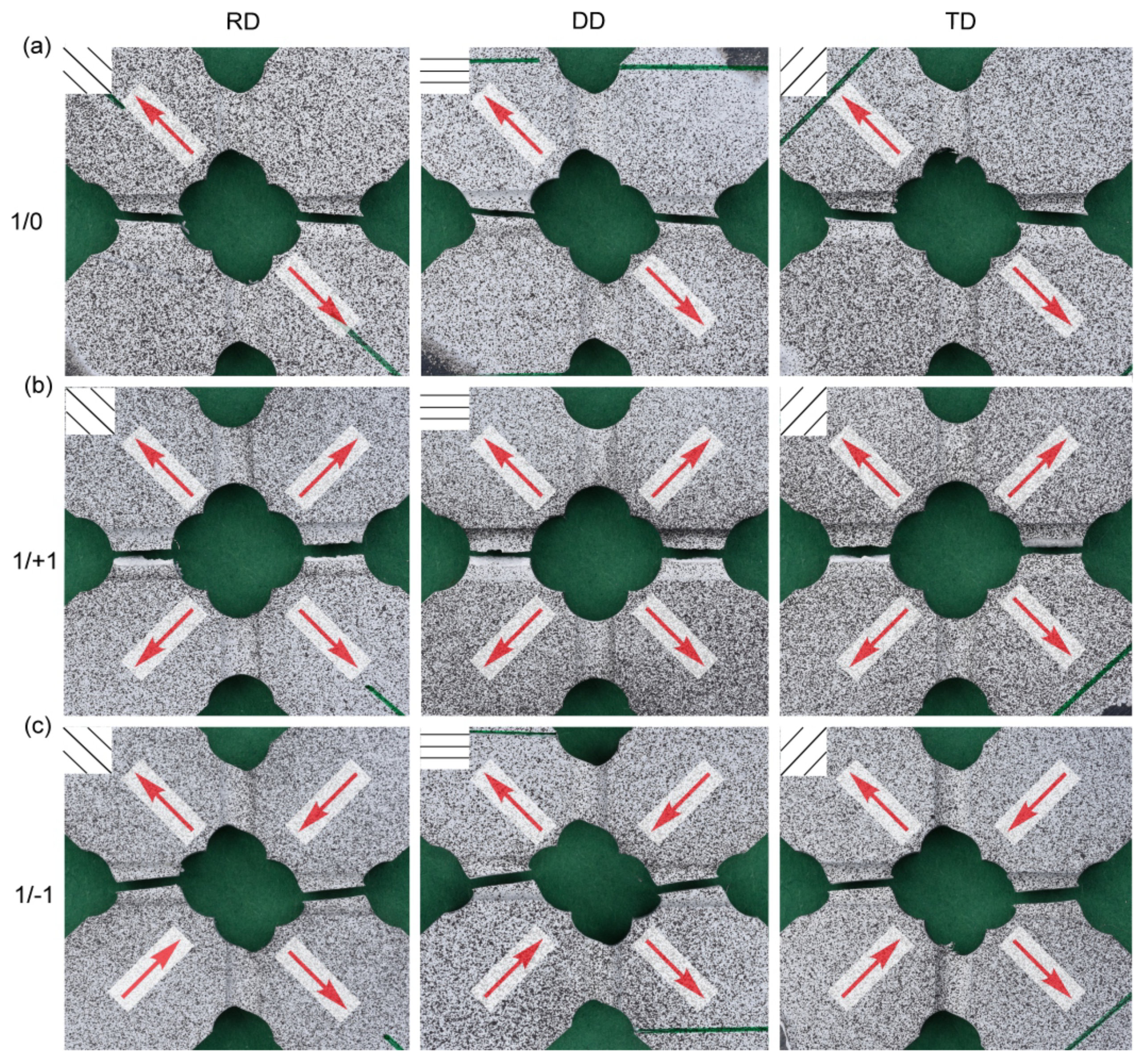
• The load ratio has an influence on the localization and orientation of principal strain bands. For moderate and zero stress triaxialities, larger strains occur for loading in DD, also indicating the more ductile behavior.
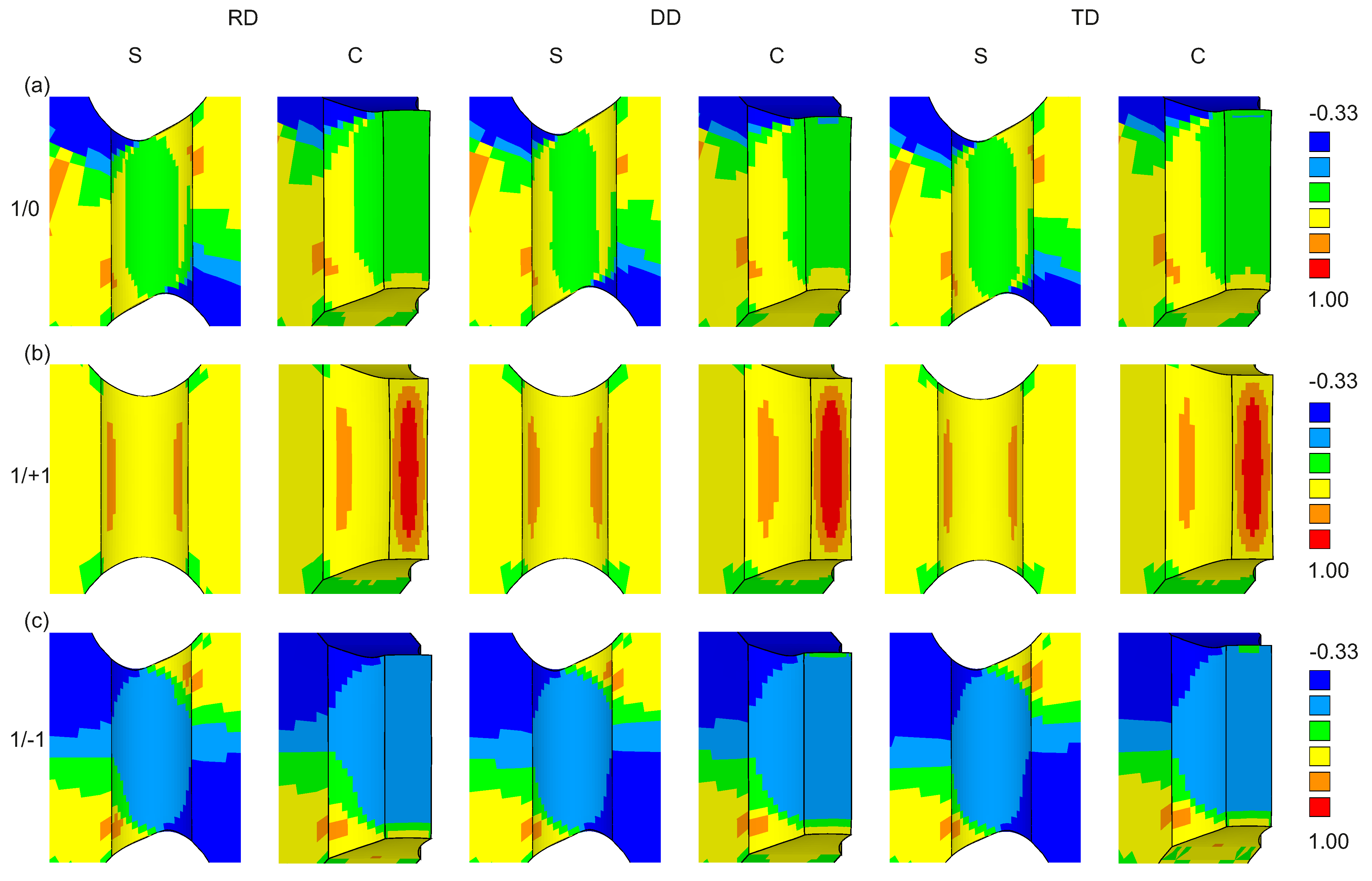
• The load ratio affects the macroscopic stresses, whereas the influence of the loading direction is marginal. A wide range of stress states can be covered by the X0 specimen under different biaxial loading conditions.
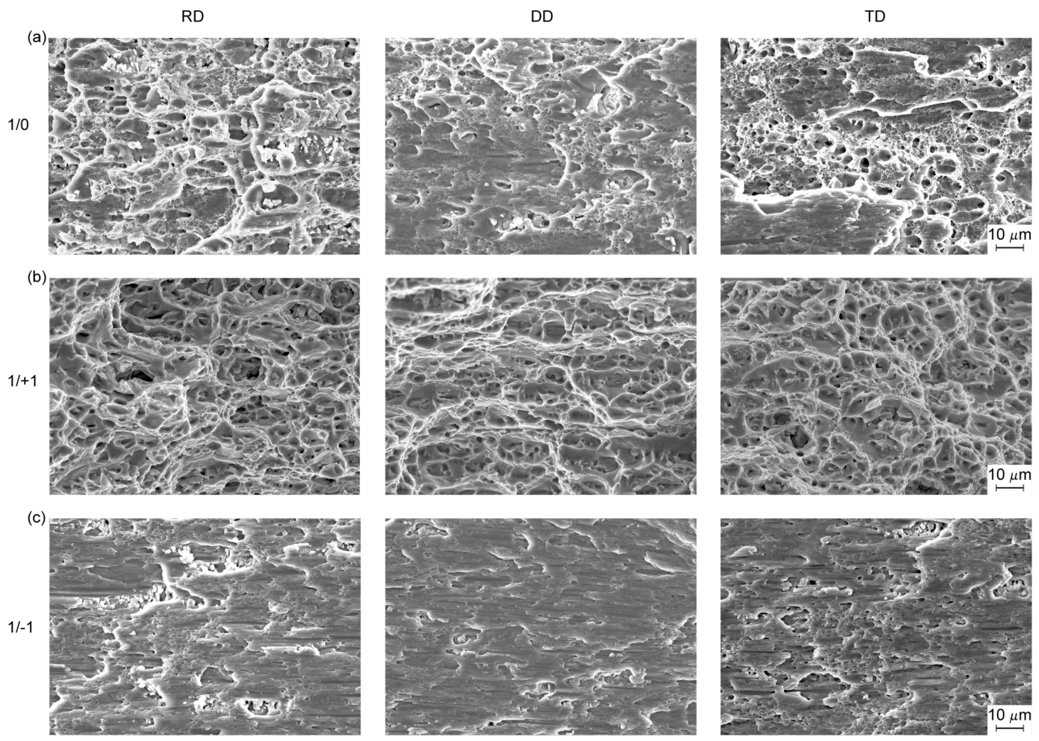
• Damage and fracture processes on the micro-scale are influenced by the load ratio and the loading direction. Loading in DD leads to more micro-shear cracks, whereas during loading in RD and TD, more voids occur.
• The experimental results reveal important information on the damage and fracture mechanisms occurring during the loading of anisotropic materials. They can be used to develop and to validate sophisticated constitutive models to simulate the deformation and failure behavior of aeronautical structures.

References

1. Stanić, D.; Zovko Brodarac, Z.; Li, L. Influence of Copper Addition in AlSi7MgCu Alloy on Microstructure Development and Tensile Strength Improvement. Metals 2020, 10, 1623. [Google Scholar] [CrossRef]
2. Yang, G.; Kim, J.K. An Overview of High Yield Strength Twinning-Induced Plasticity Steels. Metals 2021, 11, 124. [Google Scholar] [CrossRef]
3. Mazlan, S.; Yidris, N.; Koloor, S.S.R.; Petrů, M. Experimental and Numerical Analysis of Fatigue Life of Aluminum Al 2024-T351 at Elevated Temperature. Metals 2020, 10, 1581. [Google Scholar] [CrossRef]
4. Park, H.G.; Kang, B.S.; Kim, J. Numerical Modeling and Experimental Verification for High-Speed Forming of Al5052 with Single Current Pulse. Metals 2019, 9, 1311. [Google Scholar] [CrossRef] [Green Version]
5. Brünig, M. A thermodynamically consistent continuum damage model taking into account the ideas of CL Chow. Int. J. Damage Mech. 2016, 25, 1130–1141. [Google Scholar] [CrossRef]
6. Živković, J.; Dunić, V.; Milovanović, V.; Pavlović, A.; Živković, M. A Modified Phase-Field Damage Model for Metal Plasticity at Finite Strains: Numerical Development and Experimental Validation. Metals 2021, 11, 47. [Google Scholar] [CrossRef]
7. Gerke, S.; Adulyasak, P.; Brünig, M. New biaxially loaded specimens for the analysis of damage and fracture in sheet metals. Int. J. Solids Struct. 2017, 110–111, 209–218. [Google Scholar] [CrossRef]
8. Zhang, W.; Zhu, Z.; Zhou, C.; He, X. Biaxial Tensile Behavior of Commercially Pure Titanium under Various In-Plane Load Ratios and Strain Rates. Metals 2021, 11, 155. [Google Scholar] [CrossRef]
9. Bai, Y.; Wierzbicki, T. A new model of metal plasticity and fracture with pressure and Lode dependence. Int. J. Plast. 2008, 24, 1071–1096. [Google Scholar] [CrossRef]
10. Brünig, M.; Chyra, O.; Albrecht, D.; Driemeier, L.; Alves, M. A ductile damage criterion at various stress triaxialities. Int. J. Plast. 2008, 24, 1731–1755. [Google Scholar] [CrossRef]
11. Driemeier, L.; Brünig, M.; Micheli, G.; Alves, M. Experiments on stress-triaxiality dependence of material behavior of aluminum alloys. Mech. Mater. 2010, 42, 207–217. [Google Scholar] [CrossRef]
12. Bao, Y.; Wierzbicki, T. On fracture locus in the equivalent strain and stress triaxiality space. Int. J. Mech. Sci. 2004, 46, 81–98. [Google Scholar] [CrossRef]
13. Gao, X.; Zhang, G.; Roe, C. A Study on the Effect of the Stress State on Ductile Fracture. Int. J. Damage Mech. 2010, 19, 75–94. [Google Scholar] [CrossRef]
14. Li, H.; Fu, M.W.; Lu, J.; Yang, H. Ductile fracture: Experiments and computations. Int. J. Plast. 2011, 27, 147–180. [Google Scholar] [CrossRef]
15. Dunand, M.; Mohr, D. On the predictive capabilities of the shear modified Gurson and the modified Mohr–Coulomb fracture models over a wide range of stress triaxialities and Lode angles. J. Mech. Phys. Solids 2011, 59, 1374–1394. [Google Scholar] [CrossRef]
16. Roth, C.C.; Mohr, D. Ductile fracture experiments with locally proportional loading histories. Int. J. Plast. 2016, 79, 328–354. [Google Scholar] [CrossRef]
17. Lou, Y.; Chen, L.; Clausmeyer, T.; Tekkaya, A.E.; Yoon, J.W. Modeling of ductile fracture from shear to balanced biaxial tension for sheet metals. Int. J. Solids Struct. 2017, 112, 169–184. [Google Scholar] [CrossRef]
18. Liu, Y.; Kang, L.; Ge, H. Experimental and numerical study on ductile fracture of structural steels under different stress states. J. Constr. Steel Res. 2019, 158, 381–404. [Google Scholar] [CrossRef]
19. Lin, S.B.; Ding, J.L. Experimental study of the plastic yielding of rolled sheet metals with the cruciform plate specimen. Int. J. Plast. 1995, 11, 583–604. [Google Scholar] [CrossRef]
20. Green, D.E.; Neale, K.W.; MacEwen, S.R.; Makinde, A.; Perrin, R. Experimental investigation of the biaxial behaviour of an aluminum sheet. Int. J. Plast. 2004, 20, 1677–1706. [Google Scholar] [CrossRef]
21. Kuwabara, T. Advances in experiments on metal sheets and tubes in support of constitutive modeling and forming simulations. Int. J. Plast. 2007, 23, 385–419. [Google Scholar] [CrossRef]
22. Kulawinski, D.; Nagel, K.; Henkel, S.; Hübner, P.; Fischer, H.; Kuna, M.; Biermann, H. Characterization of stress–strain behavior of a cast TRIP steel under different biaxial planar load ratios. Eng. Fract. Mech. 2011, 78, 1684–1695. [Google Scholar] [CrossRef]
23. Demmerle, S.; Boehler, J.P. Optimal design of biaxial tensile cruciform specimens. J. Mech. Phys. Solids 1993, 41, 143–181. [Google Scholar] [CrossRef]
24. Song, X.; Leotoing, L.; Guines, D.; Ragneau, E. Characterization of forming limits at fracture with an optimized cruciform specimen: Application to DP600 steel sheets. Int. J. Mech. Sci. 2017, 126, 35–43. [Google Scholar] [CrossRef]
25. Liedmann, J.; Gerke, S.; Barthold, F.J.; Brünig, M. Shape optimization of the X0-specimen: Theory, numerical simulation and experimental verification. Comput. Mech. 2020, 66, 1275–1291. [Google Scholar] [CrossRef]
26. Brünig, M.; Brenner, D.; Gerke, S. Stress state dependence of ductile damage and fracture behavior: Experiments and numerical simulations. Eng. Fract. Mech. 2015, 141, 152–169. [Google Scholar] [CrossRef]
27. Brünig, M.; Zistl, M.; Gerke, S. Biaxial experiments on characterization of stress-state-dependent damage in ductile metals. Prod. Eng. 2020, 14, 87–93. [Google Scholar] [CrossRef]
28. Hill, R. A Theory of the Yielding and Plastic Flow of Anisotropic Metals. Proc. R. Soc. Lond. 1948, 193, 281–297. [Google Scholar]
29. Barlat, F.; Aretz, H.; Yoon, J.W.; Karabin, M.E.; Brem, J.C.; Dick, R.E. Linear Transformation-Based Anisotropic Yield Functions. Int. J. Plast. 2005, 21, 1009–1039. [Google Scholar] [CrossRef]
30. Ha, J.; Baral, M.; Korkolis, Y. Plastic anisotropy and ductile fracture of bake-hardened AA6013 aluminum sheet. Int. J. Solids Struct. 2018, 155, 123–139. [Google Scholar] [CrossRef]
31. Hu, Q.; Yoon, J.W.; Manopulo, N.; Hora, P. A coupled yield criterion for anisotropic hardening with analytical description under associated flow rule: Modeling and validation. Int. J. Plast. 2021, 136, 102882. [Google Scholar] [CrossRef]
32. Stoughton, T.B.; Yoon, J.W. Anisotropic hardening and non-associated flow in proportional loading of sheet metals. Int. J. Plast. 2009, 25, 1777–1817. [Google Scholar] [CrossRef]
33. Martins, J.M.; Andrade-Campos, A.; Thuillier, S. Calibration of anisotropic plasticity models using a biaxial test and the virtual fields method. Int. J. Solids Struct. 2019, 172, 21–37. [Google Scholar] [CrossRef]
34. Lattanzi, A.; Barlat, F.; Pierron, F.; Marek, A.; Rossi, M. Inverse identification strategies for the characterization of transformation-based anisotropic plasticity models with the non-linear VFM. Int. J. Mech. Sci. 2020, 173, 105422. [Google Scholar] [CrossRef]
35. Spitzig, W.A.; Richmond, O. The effect of pressure on the flow stress of metals. Acta Metall. 1984, 32, 457–463. [Google Scholar] [CrossRef]
36. Voce, E. A practical strain-hardening function. Metallurgia 1955, 51, 219–226. [Google Scholar]
37. Brünig, M.; Zistl, M.; Gerke, S. Numerical analysis of experiments on damage and fracture behavior of differently preloaded aluminum alloy specimens. Metals 2021, 11, 381. [Google Scholar] [CrossRef]
Figure 1. View of (a) schematic draw and (b) experimental setup for the tensile tests.
Metals 11 01214 g001
Figure 2. Geometry of the tensile specimen (all dimensions in mm).
Metals 11 01214 g002
Figure 3. Experimental and numerically predicted (a) r values and (b) yield stresses.
Metals 11 01214 g003
Figure 4. (a) Experimental and (b) numerically predicted true stress–true plastic strain curves.
Metals 11 01214 g004
Figure 5. (a) Biaxial test machine, (b) lighting system and camera equipment.
Metals 11 01214 g005
Figure 6. Geometry, loadings and displacements of the X0 specimen (all dimensions in mm).
Metals 11 01214 g006
Figure 7. Finite element mesh.
Metals 11 01214 g007
Figure 8. Load-displacement curves for the load ratios (a) F 1 / F 2 = 1 / 0 , (b) F 1 / F 2 = 1/+1 and (c) F 1 / F 2 = 1/−1.
Metals 11 01214 g008
Figure 9. First principal strain fields before fracture occurs for the load ratios (a) F 1 / F 2 = 1/0, (b) F 1 / F 2 = 1/+1 and (c) F 1 / F 2 = 1 / 1 .
Metals 11 01214 g009
Figure 10. Fractured specimens for the load ratios (a) F 1 / F 2 = 1 / 0 , (b) F 1 / F 2 = 1/+1 and (c) F 1 / F 2 = 1/−1.
Metals 11 01214 g010
Figure 11. Stress triaxialities η for the load ratios (a) F 1 / F 2 = 1 / 0 , (b) F 1 / F 2 = 1/+1 and (c) F 1 / F 2 = 1/−1.
Metals 11 01214 g011
Figure 12. Scanning electron microscopy of fracture surfaces for the load ratios (a) F 1 / F 2 = 1 / 0 , (b) F 1 / F 2 = 1/+1 and (c) F 1 / F 2 = 1/−1.
Metals 11 01214 g012