RANS versus Scale Resolved Approach for Modeling Turbulent Flow in Continuous Casting of Steel

Abstract

Numerical modeling is the approach used most often for studying and optimizing the molten steel flow in a continuous casting mold. The selection of the physical model might very much influence such studies. Hence, it is paramount to choose a proper model. In this work, the numerical results of four turbulence models are compared to the experimental results of the water model of continuous casting of steel billets using a single SEN port in a downward vertical orientation. Experimental results were obtained with a 2D PIV (Particle Image Velocimetry) system with measurements taken at various cut planes. Only hydrodynamic effects without solidification are considered. The turbulence is modeled using the RANS (Realizable k-ε, SST k-ω), hybrid RANS/Scale Resolved (SAS), and Scale Resolved approach (LES). The models are numerically solved by the finite volume method, with volume of fluid treatment at the free interface. The geometry, boundary conditions, and material properties were entirely consistent with those of the water model experimental study. Thus, the study allowed a detailed comparison and validation of the turbulence models used. The numerical predictions are compared to experimental data using contours of velocity and velocity plots. The agreement is assessed by comparing the lateral dispersion of the liquid jet in a streamwise direction for the core flow and the secondary flow behavior where recirculation zones form. The comparison of the simulations shows that while all four models capture general flow features (e.g., mean velocities in the temporal and spatial domain), only the LES model predicts finer turbulent structures and captures temporal flow fluctuations to the extent observed in the experiment, while SAS bridges the gap between RANS and LES.

1. Introduction

Steel is one of the essential materials in the modern economy. To remain competitive, producers strive to optimize the steel processing route towards better use of the resources and higher quality. An important tool in this effort is the process’s digitalization, where numerical modeling and optimization play an essential role [1]. One of the most critical steps in this route is the continuous casting (CC) of steel [2].

The behavior of liquid flow in the mold affects the purity of the steel and the presence of inclusions [3]. These are the key parameters in determining the quality of steel products. Therefore, to successfully predict the performance of the CC process, it is of crucial importance to know the flow fields in the submerged entry nozzle (SEN) and the mold [4,5].

Measurements of the flow field in the CC process are extremely difficult or even impossible due to high temperatures and the non-transparency of steel. Numerical models can therefore be used to study phenomena and flow behavior in the mold. The numerical simulations of CC of steel are very complex, computationally expensive, and time-consuming, so water models were often used in recent years. Due to the similar kinematic viscosity of water and steel, a numerical water model that imitates steel flow during CC can be used [6].

In many of the recent studies [5,7,8], the performance of Reynold’s Averaged Navier-Stokes (RANS) models was examined when predicting the flow in experimental water models of continuous casters. However, with the computational power being more accessible, one can afford to resolve more than just a single turbulence scale, as in the case of RANS. Scale Adaptive Simulation (SAS), with its capability to resolve at least some of the turbulence scales, bridges the gap between the RANS approach and Large Eddy Simulation (LES) approach in terms of how much of the turbulence spectrum is being resolved as opposed to being modeled [9,10,11].

Previously [12], the performance of three different turbulence models, Realizable k-ε, SST k-ω, and Scale Adaptive Simulation (SAS), was compared. It was found that models can predict general flow behavior and average velocities; however, only the SAS proved to capture at least some turbulence scales. For an in-depth understanding of the casting process, more insight into the instantaneous flow characteristics is needed. To further investigate the temporal solution of the flow field, a Scale Resolved approach is needed that resolves a part of the turbulence spectrum (larger scales) and models the rest. For this task, LES Wall-Adapting Local Eddy-Viscosity (WALE) model is used. The scope of this study aims to find the performance and feasibility of different turbulence models such as RANS, SAS, and LES for predicting the flow field in CC of steel billets. The models are rated based on agreement with PIV data from water model experiments.

2. Materials and Methods

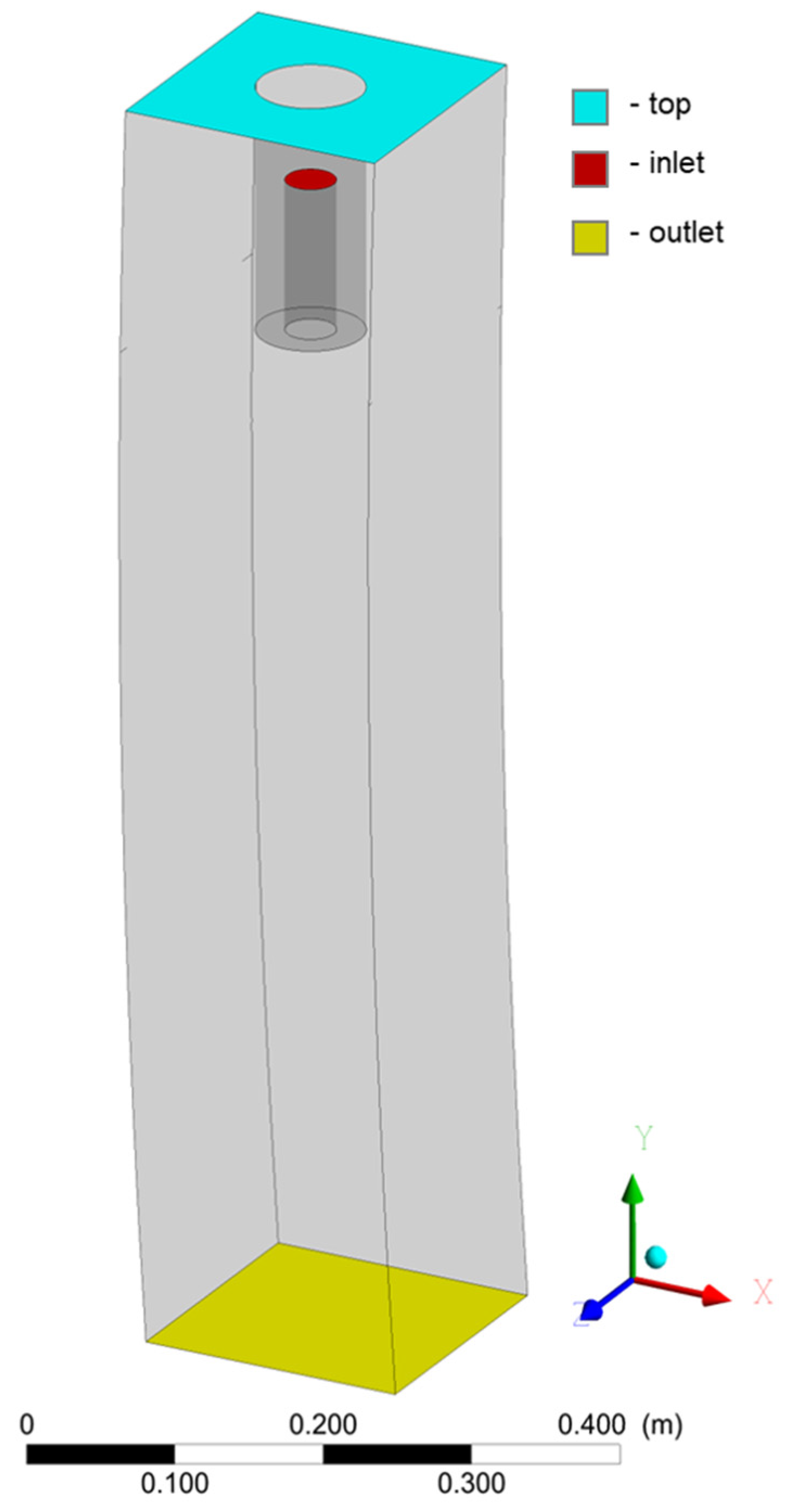
2.1. Numerical Setup and Procedure

In the numerical study that follows, the performance of the RANS, SAS, and LES approaches to modeling turbulence in a continuous steel caster are investigated.

2.1.1. Governing Equations

The flow in this study is assumed to be turbulent, incompressible, two-phase (gas and liquid with a free surface in-between), isothermal and unsteady. Therefore, mass conservation reduces to the conservation of volume fraction (given by Equation (1)), and momentum conservation reduces to Equation (2).

$$\begin{array}{c}\frac{\partial {\alpha }_L}{\partial t}+\mathbf{\nabla }·\left({\alpha }_L\mathbf{V}\right)=0\\ {\alpha }_L+{\alpha }_G=1\end{array}$$

(1)

$$\frac{\partial }{\partial t}\left(\rho V\right)+\mathbf{\nabla }·\left(\rho VV\right)=-\mathbf{\nabla }p+\mathbf{\nabla }·\mathbf{\tau }+\rho \mathit{g}$$

(2)

where V represents velocity, $\alpha$ is volume fraction, $\rho$ is density, $\tau$ is shear stress, $\rho \mathit{g}$ is the force of gravity and subscripts L and G denote liquid and gas phase, respectively. Shear stress is defined as:

$$\mathbf{\tau }=\mu \left[\left(\nabla V+\nabla V^T\right)-\frac{2}{3}\left(\nabla ·V\right)I\right],$$

(3)

where $\mu$ is dynamic viscosity, $I$ is the unit tensor and the term $\frac{2}{3}\left(\nabla ·V\right)I$ takes into account the effect of the volume dilatation.

The interface tracking of the free surface between gas and liquid was performed by the Volume of Fluid (VOF) model using an algebraic approach. The surface tension effects were neglected. Density and viscosity were computed for each cell based on the volume fraction by using Equation (4).

$$\begin{array}{c}\rho ={\alpha }_G{\rho }_G+\left(1-{\alpha }_G\right){\rho }_L\\ \mu ={\alpha }_G{\mu }_G+\left(1-{\alpha }_G\right){\mu }_L\end{array}$$

(4)

2.1.2. Turbulence Modelling

Four different approaches to turbulence modeling were considered in this study: Approach 1 (A1): Realizable k-ε model [13] with Enhanced wall treatment (Rk-ε EWT) (RANS), Approach 2 (A2): Shear Stress Transport (SST) k-ω model (RANS) [14], Approach 3 (A3): SAS model (hybrid RANS/Scale Resolved) [15] and Approach 4 (A4): Wall-Adapting Local Eddy-Viscosity (WALE) LES model (Scale Resolved) [16].

The RANS class of models uses time averaging of Navier-Stokes equations, modeling all of the turbulence scales. The variables are defined as the sum of the time-averaged value $\overline{\varphi }$ and a fluctuating value ${\varphi }^{\prime }$ (Equation (5)), while LES modeling provides an alternative approach using spatial filtering (given by Equation (1)) of the time-dependent Navier-Stokes equations, where large eddies are being resolved (not modeled). The error introduced by LES turbulence modeling can be reduced compared to RANS since most of the turbulence is being resolved and less is being modeled.

$${\varphi }_{RANS}\left(x\right)={\overline{\varphi }}_{RANS}\left(x\right)+{\varphi }_{RANS}^{\prime }\left(x\right)$$

(5)

$${\varphi }_{LES}\left(x\right)={\tilde{\varphi }}_{LES}\left(x\right)+{\varphi }_{LES}^{\prime }\left(x\right)$$

(6)

The mean value in RANS is defined by:

$${\overline{\varphi }}_{RANS}\left(x_i\right)=\underset{T\to \infty }{\lim }\frac{1}{T}{{\displaystyle \int }}_0^T\varphi \left(x_i, t\right) dt,$$

(7)

where T is the averaging interval.

The filtered values in LES are defined by:

$${\tilde{\varphi }}_{LES}\left(x\right)={{\displaystyle \int }}_D^{}\varphi \left(x^{\prime }\right)G\left(x,x^{\prime }\right)d{x}^{\prime },$$

(8)

where D is the filtering domain, and G is the filter function [17].

In A4, the filtering operation (given by Equation (9)) was determined by a finite-volume discretization solver, where V is the volume of a computational cell. The role of filtering is to separate the computational domain into two parts, the large eddies that are being resolved and the smaller eddies that are being modeled.

$${\tilde{\varphi }}_{LES}\left(x\right)=\frac{1}{V}{{\displaystyle \int }}_{\nu }^{}\varphi \left(x^{\prime }\right) d{x}^{\prime }, x^{\prime }\in \nu .$$

(9)

The implied filter function $G\left(x,x^{\prime }\right)$ is defined as:

$$G\left(x,x^{\prime }\right)=\{\begin{array}{cc}\hfill 1/V,& x^{\prime }\in \nu \hfill \\ \hfill 0,& x^{\prime } \mathrm{otherwise}\hfill \end{array}.$$

(10)

The momentum equations that are being solved can be written similarly for both LES and RANS models:

$$\frac{\partial }{\partial t}\left(\rho {\overline{u}}_i\right)+\frac{\partial }{\partial x_j}\left(\rho {\overline{u}}_i{\overline{u}}_j\right)=-\frac{\partial \overline{p}}{\partial x_j}+\frac{\partial }{\partial x_j}\left[\mu \left(\frac{\partial {\overline{u}}_i}{\partial x_j}+\frac{\partial {\overline{u}}_j}{\partial x_i}\right)\right]+\frac{\partial {\overline{\tau }}_{ij}}{\partial x_j},$$

(11)

$$\frac{\partial }{\partial t}\left(\rho {\tilde{u}}_i\right)+\frac{\partial }{\partial x_j}\left(\rho {\tilde{u}}_i{\tilde{u}}_j\right)=-\frac{\partial \tilde{p}}{\partial x_j}+\frac{\partial }{\partial x_j}\left[\mu \left(\frac{\partial {\tilde{u}}_i}{\partial x_j}+\frac{\partial {\tilde{u}}_j}{\partial x_i}\right)\right]+\frac{\partial {\tau }_{ij}^s}{\partial x_j}.$$

(12)

The large eddies are resolved by direct numerical solution of the Navier-Stokes equations (Equation (13)).

$$\frac{\partial }{\partial t}\left(\rho u_i\right)+\frac{\partial }{\partial x_j}\left(\rho u_i{u}_j\right)=-\frac{\partial p}{\partial x_j}+\frac{\partial }{\partial x_j}\left[\mu \left(\frac{\partial u_i}{\partial x_j}+\frac{\partial u_j}{\partial x_i}\right)\right]$$

(13)

RANS and LES equations have the same general form as the instantaneous Navier-Stokes equations. The velocities and other solution variables subsequently represent time-averaged values in RANS and filtered values in the LES model. The term ${\tau }_{ij}$ needs to be modeled and can be defined as Reynolds stresses (Equation (14)) for RANS or sub-grid-scale Reynolds stresses (Equation (15)) for the LES approach.

$${\overline{\tau }}_{ij}=-\rho \overline{{u^{\prime }}_i{u^{\prime }}_j}={\mu }_t\left(\frac{\partial {\overline{u}}_i}{\partial x_j}+\frac{\partial {\overline{u}}_j}{\partial x_i}\right)+\frac{2}{3}\rho {\delta }_{ij}k$$

(14)

$${\tau }_{ij}^s=-\rho \left(\overline{u_i{u}_j}-\overline{u_i}\overline{u_j}\right)={\mu }_t\left(\frac{\partial {\overline{u}}_i}{\partial x_j}+\frac{\partial {\overline{u}}_j}{\partial x_i}\right)+\frac{1}{3}{\tau }_{kk}^s{\delta }_{ij}$$

(15)

Eddy viscosity ${\mu }_t$ for RANS models can be expressed for A1 model as

$${\mu }_t=\rho C_{\mu }\frac{k^2}{ϵ},$$

(16)

And for A2 and A3 models as

$${\mu }_t=\rho \frac{k}{\omega }\frac{1}{\max \left[\frac{1}{{\alpha }^{*}},\frac{S{F}_2}{a_1\omega }\right]}.$$

(17)

The RANS turbulence models considered in the present scope belong to the two-equation class, where an additional set of transport equations are solved. These additional equations include the turbulence kinetic energy (k) and its dissipation rate (ε)/specific dissipation rate (ω). The general transport Equation (18) for k is similar for all three models. In the case of A1, A2, and A3, the production term for k due to mean velocity gradient (G_k) is the same, while the production terms due to buoyancy (G_b) is 0 for A2 and A3.

$$\frac{\partial }{\partial \mathrm{t}}\left(\rho k\right)+\frac{\partial }{\partial {\mathrm{x}}_{\mathrm{j}}}\left(\rho k{u}_j\right)=\frac{\partial }{\partial {\mathrm{x}}_{\mathrm{j}}}\left(\left(\mu +\frac{{\mu }_t}{{\sigma }_k}\right)\frac{\partial \mathrm{k}}{\partial {\mathrm{x}}_{\mathrm{j}}}\right)+G_k+G_b-Y_k$$

(18)

Transport of ε is given by Equation (19) for A1, while in the case of A2 and A3, ω transport is represented by Equations (20) and (21). The difference between these equations is that G_b,ε term (dissipation production due to buoyancy) is only present in ε Equation (19), and D_ω (cross-diffusion modification) term is only present in both ω based models. The latter allows the blending of standard k-ω and the standard k-ε approach.

$$\frac{\partial }{\partial \mathrm{t}}\left(\rho ϵ\right)+\frac{\partial }{\partial {\mathrm{x}}_{\mathrm{j}}}\left(\rho ϵu_j\right)=\frac{\partial }{\partial {\mathrm{x}}_{\mathrm{j}}}\left(\left(\mu +\frac{{\mu }_t}{{\sigma }_{ϵ}}\right)\frac{\partial ϵ}{\partial {\mathrm{x}}_{\mathrm{j}}}\right)+G_{ϵ}+G_{b,ϵ}-Y_{ϵ}$$

(19)

$$\frac{\partial }{\partial \mathrm{t}}\left(\rho \omega \right)+\frac{\partial }{\partial {\mathrm{x}}_{\mathrm{j}}}\left(\rho \omega u_j\right)=\frac{\partial }{\partial {\mathrm{x}}_{\mathrm{j}}}\left(\left(\mu +\frac{{\mu }_t}{{\sigma }_{\omega }}\right)\frac{\partial \mathsf{\omega }}{\partial {\mathrm{x}}_{\mathrm{j}}}\right)+G_{\omega }-Y_{\omega }+D_{\omega }$$

(20)

$$\frac{\partial }{\partial \mathrm{t}}\left(\rho \omega \right)+\frac{\partial }{\partial {\mathrm{x}}_{\mathrm{j}}}\left(\rho \omega u_j\right)=\frac{\partial }{\partial {\mathrm{x}}_{\mathrm{j}}}\left(\left(\mu +\frac{{\mu }_t}{{\sigma }_{\omega }}\right)\frac{\partial \mathsf{\omega }}{\partial {\mathrm{x}}_{\mathrm{j}}}\right)+G_{\omega }-Y_{\omega }+D_{\omega }+Q_{SAS}$$

(21)

The Equations (20) and (21) for A2 and A3 are principally the same, except for the term Q_SAS. The Q_SAS term incorporates the von Karman length scale into the A3, allowing it to alter the turbulence length scales to the already resolved scales. In principle, this means that the model can resolve the additional turbulence structures down to the grid spacing, making it a hybrid between the RANS and the LES.

In LES simulation, the Wall-Adapting Local Eddy-Viscosity (WALE) model was used to model eddy viscosity (Equation (22)), where $L_s$ is the mixing length for sub-grid scales, ${\overline{S}}_{ij}$ is the rate-of-strain tensor for the resolved scale and $S_{ij}^d$ is defined as $\frac{\partial {\overline{u}}_i}{\partial x_j}$ [16].

$${\mu }_t = \rho L_s^2\frac{{\left(S_{ij}^d{S}_{ij}^d\right)}^{3/2}}{{\left({\overline{S}}_{ij}{\overline{S}}_{ij}\right)}^{5/2}+{\left(S_{ij}^d{S}_{ij}^d\right)}^{5/4}}$$

(22)

Detailed information about the involved terms, implementation, and usage can be found in [13,14,15,16,18].

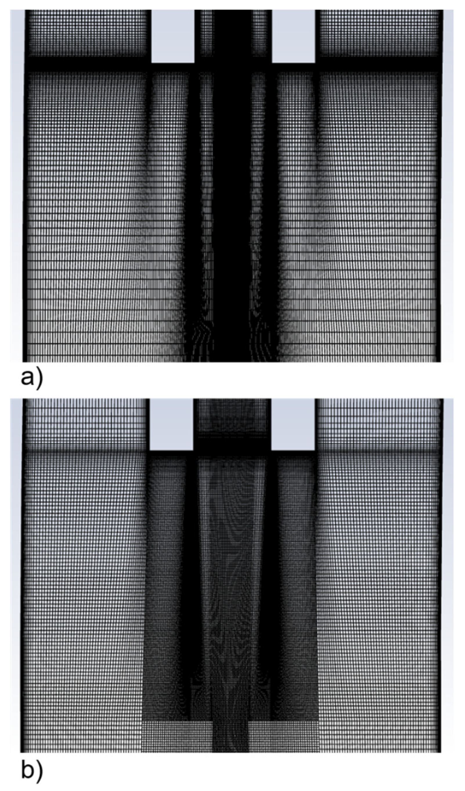
2.1.3. Discretization

To validate the numerical outcomes, the geometry was designed based on the experimental test section of the water model, which is a 1:1 copy of the industrial caster used by our industrial partner. Minor changes in the geometry were made to reduce the total number of computational cells in the upper part of the mold, while the geometry of the region of primary interest was not changed.

A 3D computational domain (Figure 1) is considered to be the same as used in the experimental model. The spatial discretization is carried out by ensuring maximum refinement in the region of expected large gradients of flow fields.

For RANS and SAS models, a matching mesh with 3,247,842 computational cells is used (Figure 2b). For LES simulation, the discretization procedure was changed to non-matching. With such an approach, additional refinements were made that allowed resolving of 80% of the turbulence spectrum while still maintaining a reasonable cell count of 5,529,888 computational cells (Figure 2a). A butterfly grid structure, which generally provides the best grid quality for cylindrical geometries in terms of orthogonality and mesh density, was constructed for both meshes. Mesh refinements for the LES model were considered based on the computed SST k-ω model.

2.1.4. Boundary Conditions and Solution Procedure

Four different areas were defined for applying boundary conditions: inlet, outlet, top, and wall. The velocity field in the SEN was calculated by a separate simulation of fluid flow. This serves to define the flow conditions at the outlet of SEN. Outlet and top were defined as pressure outlet, where the gauge pressure at the outlet was set to the value which kept the free surface at the proper position, and the gauge pressure on the top was set to 0 Pa. Stationary wall with the no-slip condition was used as a boundary condition on the wall.

Water and air were used for the liquid and gaseous phase, respectively. Their properties are summarized in

Table 1. Material properties for similarity analysis.

Material	Density (kg·m−3)	Dynamic Viscosity (kg·m−1·s−1)
Water (liquid)	0.9982 × 10+3	1.003 × 10−3
Air (gas)	1.2250 × 10+3	1.820 × 10−5
Steel (liquid)	6.8839 × 10+3	5.318 × 10−3

.

The temporal discretization was done using the second-order implicit formulation for RANS models and bounded second-order implicit formulation for the LES model. Compressive scheme, Least Squares Cell Based, and PRESTO! were used for volume fraction, spatial discretization of gradients, and pressure discretization, respectively. In the case of momentum equation and turbulence quantities, the second-order upwind scheme was used for RANS models, while the bounded central differencing scheme was used for LES models. SIMPLEC algorithm was used for pressure–velocity coupling.

The numerical models described in Section 2.1 are solved using ANSYS Fluent 2020.R1 (Ansys, Inc., Canonsburg, PA, USA), which relies on the finite volume framework. The time step is between 10⁻³ and 5 × 10⁻³ s. The time step is determined by the global Courant number, which was gradually reduced and set to the value of 0.5 for the last 100 s of the simulations. The absolute convergence criteria are used with values of globally scaled residuals set to 10⁻⁴. This is satisfied at every time step.

The simulations for the RANS approach on 24 cores (AMD Opteron8439SE 2.8GHz) took ~8 days. The computational time for the LES model was significantly longer compared to RANS. The final result from the simulation using the SST k-ω model was used to initialize the LES case, which was then run on 96 cores (Intel Xeon E5-2680V3 2.5GHz) for approximately 50 days.

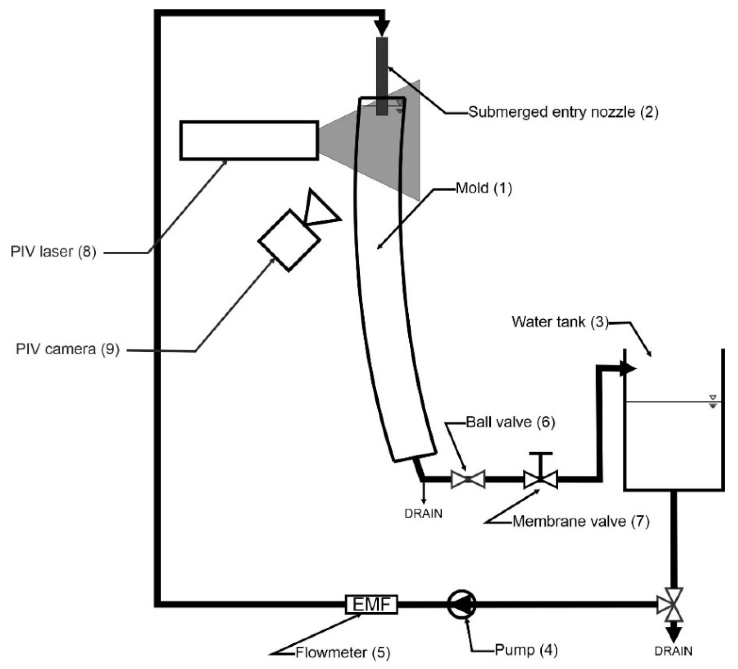
2.2. Experimental Setup and Methods

Experimental data play an essential role in understanding how flow behaves. It is usually the center-stone for the validation of any newly developed numerical model.

Our experimental test section is based on an industrial caster for steel billets used by the Štore Steel company in Slovenia. The mold itself is designed from a transparent 8 mm thick polycarbonate. The inner cross-section is square with a size of 190 mm × 190 mm. In the casting direction (vertical), the mold is curved, as shown in Figure 3. The SEN tip, also made from polycarbonate, has a diameter of 35 mm and 65 mm on the inside and outside, respectively. The length of the SEN tip is 300 mm. A straight stainless-steel pipe with an inner diameter of 35 mm and length of 1.2 m is connected to the SEN tip in the upstream direction. They form a 1.5 m long straight pipe section with a constant inner diameter to allow undisrupted flow development.

A complete experimental loop is schematically presented in Figure 3. Water is held in the tank (3) that is connected to the pump (Grundfos/CRNE16) (4). The pump, which is frequency controlled, is used to regulate the flowrate to the desired value held by the flowmeter (Enderss + Hauser/Promag F) (5). Water flows along plastic conduits and enters the SEN (2) at the top of the system. Through a straight vertical SEN, the flow gets developed before entering the mold. Two valves are positioned in line downstream of the mold. The first is a ball valve (6) used for filling the test loop and during starting and stopping. The second is a membrane valve (7), which offers a fine adjustment of free surface position at the top of the mold.

2.2.1. Experimental Conditions and Process Similarity

Experiments are performed at isothermal ambient conditions. As a consequence, all thermal effects are disregarded.

A flow similarity study between real-life conditions with molten steel and laboratory measurements using water was carefully performed to assure the relevance of the results. A typical industrial casting speed of 1.4 m/min was used as the input parameter at which tests were performed. Firstly, the flow rate of material through industrial caster was estimated, using casting speed as mentioned above and the casters cross-section. The shrinkage during solidification was not considered. Secondly, the steel flow Reynolds number was calculated based on the flow rate of material through the mold, dimensions of mold, and steel properties at casting conditions. Lastly, the water flow rate was calculated using the Reynolds number of steel and material properties of water at ambient conditions. The resulting mean velocity at the end of the SEN is 1.02 m/s. The materials and their properties are summarized in Table 1.

2.2.2. PIV Measurements

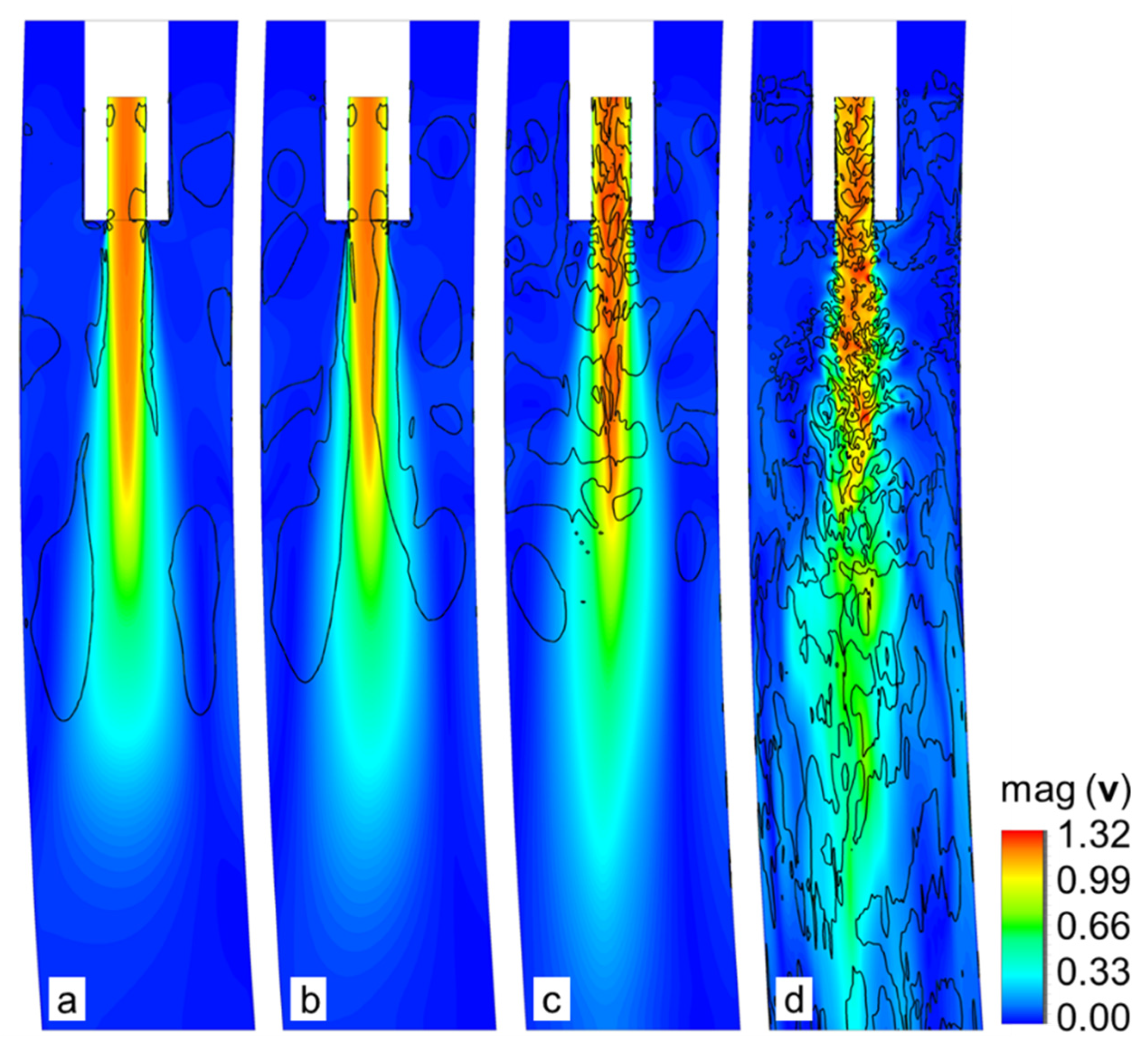
2D Particle Image Velocimetry (PIV) system from Dantec Dynamics was chosen for velocity measurements. For seeding, encapsulated rhodamine was used. The size of the particles was 10 μm. Particles were recorded with a 4Mpix double exposure camera (9) with high sensitivity sensor. The operating frequency of the system was set to 15 Hz, which, combined with 10 s long measurements, yields 150 velocity fields per measurement. The particles were illuminated with a pulsed laser (8) capable of delivering 65 mJ at 532 nm wavelength. The time difference between two successive pulses was 1.7 ms. System control and data post-processing were done in DynamicStudio software (Dantec Dynamics, Skovlunde, Denmark).

3. Results

The first task is to estimate the agreement between the results of numerical simulation and experimental measurements. This is done via comparison of velocity contours in two separate planes; x-y (Figure 4) plane and y-z (Figure 5) plane. In both cases, the plane cuts through the middle of the SEN. In the numerical simulation, the results are taken from the 214th second and represent instantaneous values, while experimental results show one randomly picked velocity field from the time series.

All four models capture the basic shape of the main jet exiting the SEN in a similar manner, as can be seen from Figure 4 and Figure 5. In the case of RANS models (A1 and A2), the velocity field is steady, and the jet exiting the SEN is symmetrical to the SEN axis. In the case of A3, the general shape of velocity contours resembles the results of A1 and A2. Still, one can see more minor variations in velocity magnitude, especially in the core flow and in the near-wall region. This is due to the fact that A3 can adjust the von Karman length scale and consequently capture at least a small portion of turbulent scales. Additionally, a steady-state solution could not be achieved using A3. In the results of A4, one can see a significant step up from previous results in terms of structures that are predicted. The A4 model shows proper “turbulence-like” behavior that is very much in line with experimental observations.

Note that experimental contour plots contain certain regions where local velocity seems to be unphysical/unexpected (near the interface or the bottom part of the image). In these regions, the results are affected by laser light scattering or week illumination at the boundaries of the observation window.

The degree of agreement between numerical simulations and experimental data is further explored by comparing y velocity component plots. The data is taken at z = 0 and plotted over the x coordinate ranging from one side of the mold to the other. The velocity profiles presented in Figure 6 correspond to two different streamwise positions; y = −50 mm (Figure 6a) and y = −150 mm (Figure 6b) from the SEN bottom with the same temporal settings used in Figure 4 and Figure 5. The general agreement is acceptable. The A1 and A2 models show very similar trends, while A3 and A4 show certain deviations, especially in the high-velocity region (the center of the mold) and in the low-velocity regions (near the wall) where the secondary flow develops. The differences are in line with the capabilities of the models; the results for A1 and A2 are averaged in temporal domain with a single length scale, and the A3 shows more »unsteadiness« in the jet core region owing to its capability to adjust its length scale locally. The closest agreement to experimental data, based on Figure 6, can be seen in the case of A4. The level of velocity variations is similar to that of the experiment in core flow, as well as in secondary flow. Note that complete overlap of plots is practically impossible as both experimental data and A4 simulation are transient. Even if one could accurately map initial experimental conditions to numerical simulation, it is not feasible to keep the simulation running in order to achieve comparable physical times. Analysis shows that A4 gives the most realistic prediction of the models being tested.

The results presented in this paper conclusively show that A4 gives the prediction closest to experimental observations. However, this fact does not make «picking a winner» any easier as a significant increase in computational effort is needed to perform A4 type simulation. This is especially true in light of the Hybrid LES-RANS approach (A3), which takes approximately ¼ of time and 40% less computational cells, yet still predicts some of the scales. It is shown here that all the tested models can decently predict the basic flow. If one is only interested in general flow structures, basic RANS performs well enough. There are situations, however, when the advantages of A3 and even more A4 come into play. If the research emphases are on the secondary flow, using typical RANS would give quite misleading results, and even more so in the case of, e.g., an inclusion path study. The inclusions are expected to be influenced by the flow. Therefore, it is necessary to resolve all the scales at which eddies are still powerful enough to affect the movement of inclusion particles. According to Figure 7, where structures in the turbulent flow are represented by iso-values of λ₂ parameter, it is clear that A4 is superior to other tested models in that respect. Still, long computational time makes this approach hard to justify in a real-life industrial purpose, where many optimizing or parameter sensitivity simulations need to be performed.

There are also other aspects of the flow field in a mold during continuous casting that were not addressed within this study, e.g., heat transfer and solidification. In reality, all these phenomena are intertwined and could not be trivially separated. Hence, it would be beneficial to test these turbulence models coupled with energy equation, possible external fields (like EM field), and solidification to gain a reasonably complete picture of the actual industrial situation.

4. Conclusions

The paper deals with the assessment of different models associated with the modeling of turbulent flow in continuous casting of steel. The prediction capabilities are tested on mold geometry used for continuous casting of steel billets. The assessment is based only on a hydrodynamic description of the flow. Using a similarity analysis, the industrial process was scaled to the laboratory water model, used as a benchmark. The comparison was made against PIV velocity measurements. The key findings are:

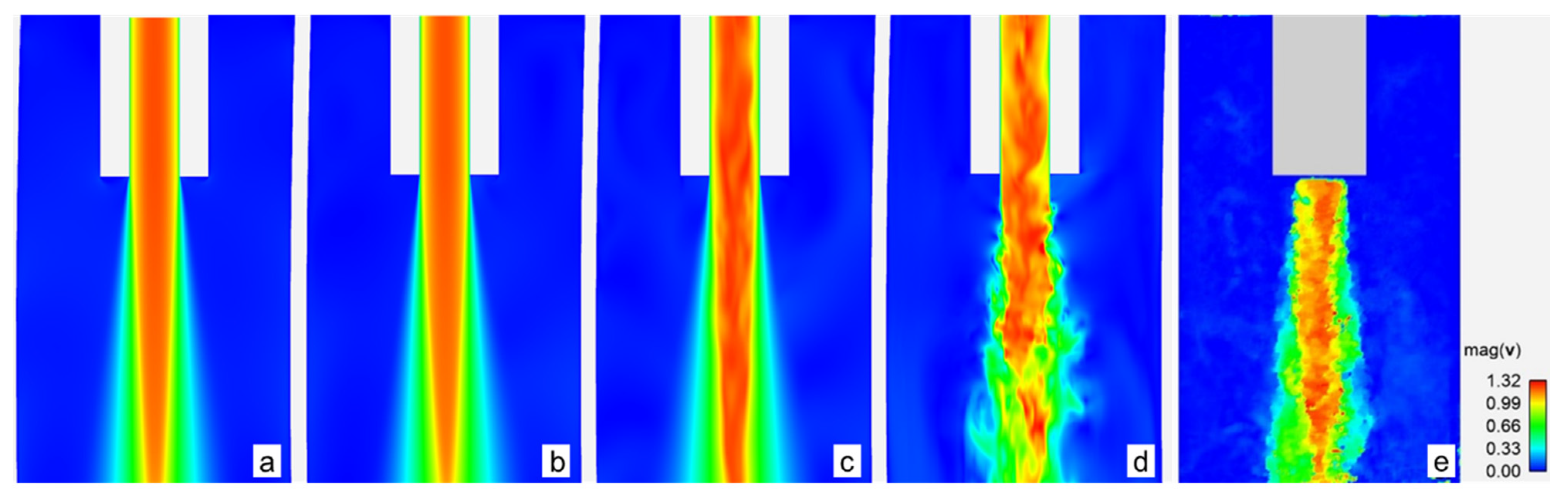
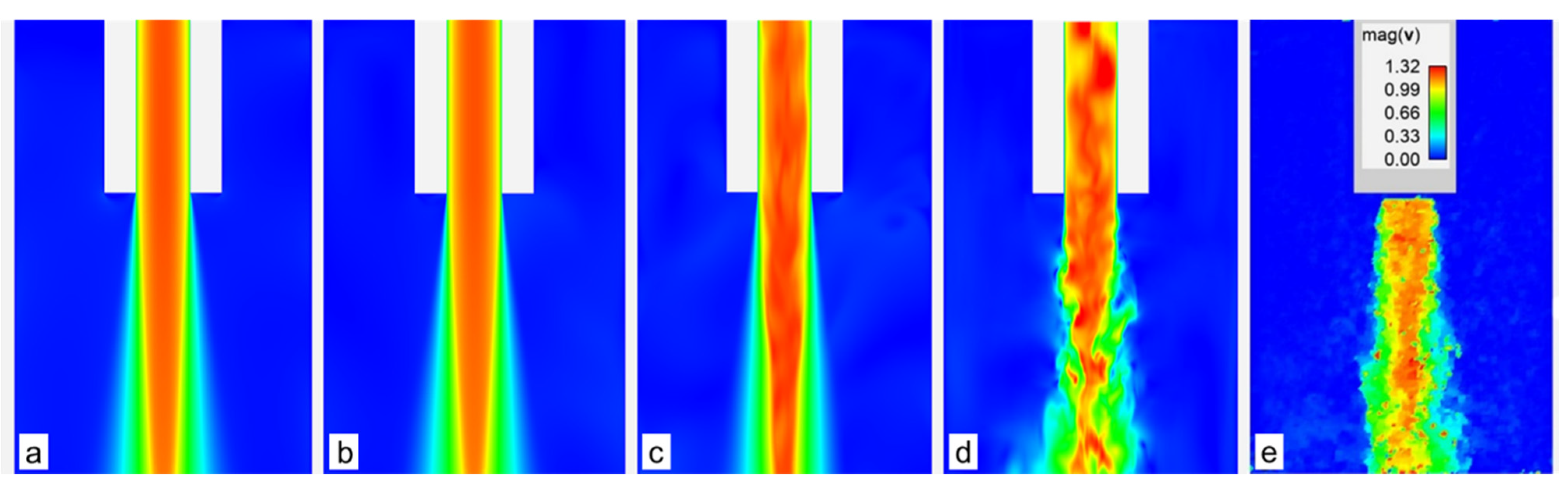
• General flow features can be reasonably predicted using either of the models.
• In the case of typical RANS models (Realizable k-ε EWT and SST k-ω), the solution is more or less steady, even if the solving procedure is transient.
• With the SAS and LES models, a steady solution does not exist. Fluctuations in the primary jet are always present.
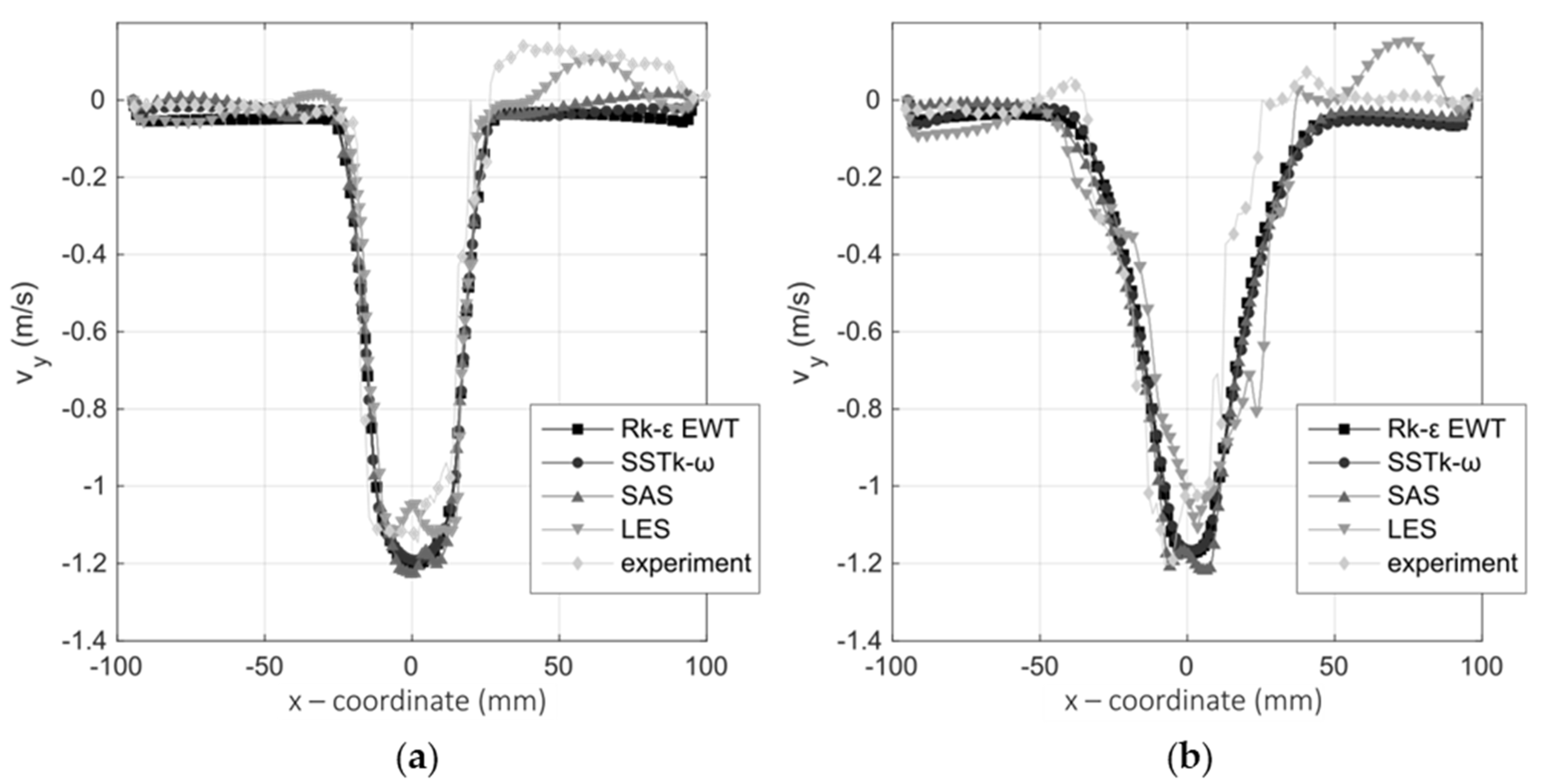
• LES model offers the closest prediction to experimental PIV data. It can also resolve secondary flow with a high degree of similarity to the experiment.
• Similar computational costs were observed for Realizable k-ε EWT and SST k-ω models. A significant increase is observed for the SAS model and even more in the case of the LES model. The computational times increase by a factor of 4, and the number of computational cells increases by a factor of 1.7 compared to the SAS model.
• An increase in computational cost is only feasible if a detailed description of the flow is needed, e.g., the study of inclusion paths.

References

1. Branca, T.A.; Fornai, B.; Colla, V.; Murri, M.M.; Streppa, E.; Schröder, A.J. The challenge of digitalization in the steel sector. Metals 2020, 10, 288. [Google Scholar] [CrossRef] [Green Version]
2. Hardin, R.A.; Liu, K.; Kapoor, A.; Beckermann, C. A transient simulation and dynamic spray cooling control model for continuous steel casting. Metall. Mater. Trans. B Process Metall. Mater. Process. Sci. 2003. [Google Scholar] [CrossRef]
3. Da Costa, E.; Silva, A.L.V. The effects of non-metallic inclusions on properties relevant to the performance of steel in structural and mechanical applications. J. Mater. Res. Technol. 2019, 8, 2408–2422. [Google Scholar] [CrossRef]
4. Väyrynen, P.; Wang, S.; Louhenkilpi, S.; Holappa, L. Modeling and removal of inclusions in continuous casting. In Proceedings of the Materials Science and Technology 2009—International Symposium on Inclusions and Clean Steel, Pittsburg, PA, USA, 25–29 October 2009. [Google Scholar]
5. Saeidy Pour, M.A.; Hassanpour, S. Steel Cleanliness Depends on Inflow Turbulence Intensity (in Tundishes and Molds). Metall. Mater. Trans. B Process Metall. Mater. Process. Sci. 2020. [Google Scholar] [CrossRef]
6. Chaudhary, R.; Rietow, B.T.; Thomas, B.G. Differences between physical water models and steel continuous casters: A theoretical evaluation. In Proceedings of the Materials Science and Technology 2009—International Symposium on Inclusions and Clean Steel, Pittsburg, PA, USA, 25–29 October 2009. [Google Scholar]
7. Chaudhary, R.; Ji, C.; Thomas, B.G.; Vanka, S.P. Transient turbulent flow in a liquid-metal model of continuous casting, including comparison of six different methods. Metall. Mater. Trans. B Process Metall. Mater. Process. Sci. 2011. [Google Scholar] [CrossRef]
8. Cho, S.M.; Thomas, B.G.; Kim, S.H. Effect of Nozzle Port Angle on Transient Flow and Surface Slag Behavior During Continuous Steel-Slab Casting. Metall. Mater. Trans. B Process Metall. Mater. Process. Sci. 2019, 50, 52–76. [Google Scholar] [CrossRef]
9. Yuan, Q.; Sivaramakrishnan, S.; Vanka, S.P.; Thomas, B.G. Computational and experimental study of turbulent flow in a 0.4-scale water model of a continuous steel caster. Metall. Mater. Trans. B Process Metall. Mater. Process. Sci. 2004. [Google Scholar] [CrossRef]
10. Ramos-Banderas, A.; Sánchez-Pérez, R.; Morales, R.D.; Palafox-Ramos, J.; Demedices-García, L.; Díaz-Cruz, M. Mathematical simulation and physical modeling of unsteady fluid flows in a water model of a slab mold. Metall. Mater. Trans. B Process Metall. Mater. Process. Sci. 2004, 35, 449–460. [Google Scholar] [CrossRef]
11. Zhao, B.; Thomas, B.G.; Vanka, S.P.; O’Malley, R.J. Transient fluid flow and superheat transport in continuous casting of steel slabs. Metall. Mater. Trans. B Process Metall. Mater. Process. Sci. 2005, 36, 801. [Google Scholar] [CrossRef] [Green Version]
12. Gregorc, J.; Kunavar, A.; Šarler, B. Performance of turbulence models for flow prediction in a mould of continuous steel caster. IOP Conf. Ser. Mater. Sci. Eng. 2020, 861, 012019. [Google Scholar] [CrossRef]
13. Shih, T.H.; Liou, W.W.; Shabbir, A.; Yang, Z.; Zhu, J. A new k-ϵ eddy viscosity model for high reynolds number turbulent flows. Comput. Fluids 1995, 24, 227–238. [Google Scholar] [CrossRef]
14. Menter, F.R. Two-equation eddy-viscosity turbulence models for engineering applications. AIAA J. 1994, 32, 1598–1605. [Google Scholar] [CrossRef] [Green Version]
15. Menter, F.R.; Egorov, Y. The scale-adaptive simulation method for unsteady turbulent flow predictions. part 1: Theory and model description. Flow Turbul. Combust. 2010, 85, 113–138. [Google Scholar] [CrossRef]
16. Ducros, F.; Nicoud, F.; Poinsot, T. Wall-adapting local eddy-viscosity models for simulations in complex geometries. Conf. Numer. Methods Fluid Dyn. 1998, 6, 293–299. [Google Scholar]
17. Ferziger, J.H.; Perić, M.; Street, R.L. Computational Methods for Fluid Dynamics, 4th ed.; Springer International Publishing: Cham, Switzerland, 2020. [Google Scholar]
18. ANSYS. User Guide for ANSYS 18.2; ANSYS Inc.: Cotonsburg, PA, USA, 2015. [Google Scholar]
Figure 1. The geometry of the computational model.
Metals 11 01140 g001
Figure 2. Comparison of the mesh for LES (a) and RANS (b) models in the x-y plane.
Metals 11 01140 g002
Figure 3. A schematic representation of the test rig.
Metals 11 01140 g003
Figure 4. Contours of velocity magnitude in the x-y plane at z = 0 (middle of the SEN) for A1 (a), A2 (b), A3 (c), A4 (d), and experiment (e).
Metals 11 01140 g004
Figure 5. Contours of velocity magnitude in the y-z plane at z = 0 (middle of the SEN) for A1 (a), A2 (b), A3 (c), A4 (d), and experiment (e).
Metals 11 01140 g005
Figure 6. Velocity vy vs. x coordinate at z = 0 and y = −50 mm (a), and y = −150 mm (b).
Metals 11 01140 g006
Figure 7. Turbulent structures represented as iso-values of λ2 = −0.15 s−2 on top of the velocity magnitude contours on the x-y plane at z = 0 m for A1 (a), A2 (b), A3 (c), and A4 (d).
Metals 11 01140 g007