Multiphasic Study of Fluid-Dynamics and the Thermal Behavior of a Steel Ladle during Bottom Gas Injection Using the Eulerian Model

Abstract

In this work, the fluid dynamic and thermal behavior of steel was analyzed during argon gas stirring in a 140-t refining ladle. The Eulerian multiphase mathematical model was used in conjunction with the discrete ordinates (DO) thermal radiation model in a steel-slag-argon system. The model was validated by particle image velocimetry (PIV) and the analysis of the opening of the oil layer in a physical scale model. The effect of Al₂O₃ and Mg-C as a refractory in the walls was studied, and the Ranz-Marshall and Tomiyama models were compared to determine the heat exchange coefficient. The results indicated that there were no significant differences between these heat exchange models; likewise, the radiation heat transfer model adequately simulated the thermal behavior according to plant measurements, finding a thermal homogenization time of the steel of 2.5 min for a gas flow of 0.45 Nm³·min⁻¹. Finally, both types of refractory kept the temperature of the steel within the ranges recommended in the plant; however, the use of Al₂O₃ had better heat retention, which would favor refining operations.

1. Introduction

Secondary refining is the process of making steel where it is chemically adjusted to obtain the desired quality. Synthetic slag is commonly used for the removal or reduction of unwanted elements and compounds. The enhancement of chemical reactions between slag and steel compounds occurs using the injection of argon gas [1,2]. Various studies have shown that the fluid dynamics structure [3,4,5,6,7], the mass transfer [8,9], and the chemical reaction rates [10] are affected by the flow of injected gas. In addition, gas stirring helps to eliminate temperature gradients in steel [11,12] generated mainly by exothermic reactions, the heat losses through the ladle walls, electrode reheating, and the ladle residence time [13]. Computational fluid dynamics (CFD) is a technique that helps to analyze the effect of variables such as temperature in the metallurgical process and is currently one of the most used techniques [12,14,15,16,17]. The thermal control of secondary refining is an important process because it affects the deoxidation and desulfurization processes, as well as the rate of chemical reactions [18]. The use of numerical and experimental modeling in secondary refining has been used to study the heat loss of the steel through the walls of the ladle [19], during the holding period in the furnace [20,21,22,23], the casting to the tundish (teeming) [24,25], as well as the thermal mixing of steel [26]. Castillejos et al. [27] studied the process of thermal homogenization of steel using gas agitation and concluded that after 3 min, the temperature is completely homogeneous.

It has also been shown that the slag layer, in addition to modifying the fluid dynamics structure [9], works as an insulating layer that prevents heat losses in the surface mainly due to the radiation mechanism [14]. In the present work, the CFD technique was used for the complete study of the fluid dynamics and thermal behavior of steel in a metallurgical ladle during argon gas stirring. The Euler-Euler approach was used with drag and non-drag forces using the Eulerian multiphase model, and the Ranz-Marshall [28] and Tomiyama [29] models were compared to calculate the heat exchange coefficient. The fluid dynamics results were validated by means of a physical scale model using the particle image velocimetry (PIV) technique and analysis of the opening of the oil layer. For the calculation of heat losses by radiation, the discrete ordinates (DO) radiation model was used, and the results were compared with those obtained with different methodologies. Finally, the effects of two refractories commonly used in the industry on the variation of the global temperature of steel were compared.

2. Materials and Methods

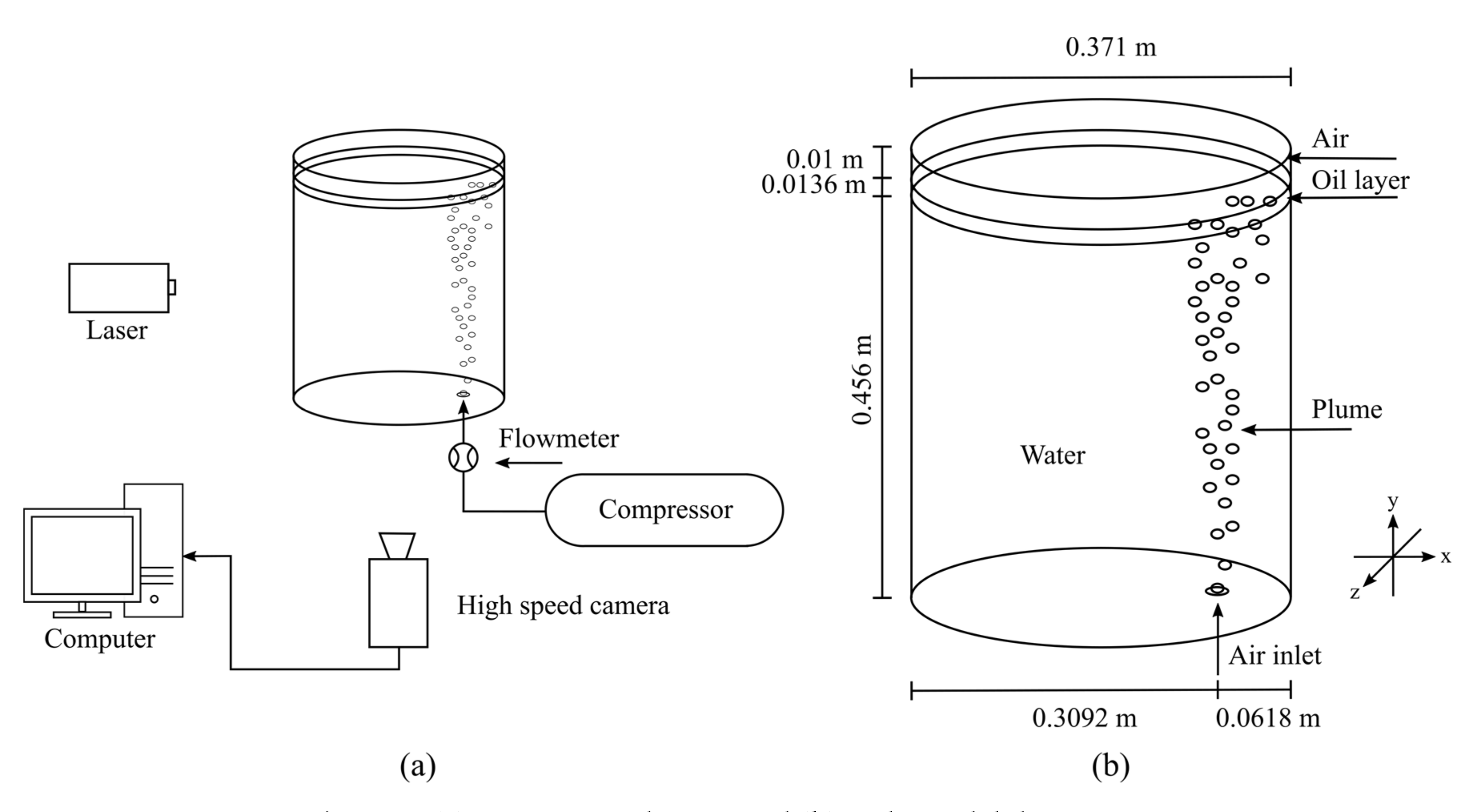
2.1. Physical Modeling

The experimentation was carried out on a 1:7-scale acrylic model of the ladle furnace using water, synthetic oil Mobil DTE 24^® (ExxonMobil, Mexico City, Mexico) and air to emulate steel, slag, and argon, respectively. To carry out the stirring, air was injected by means of a nozzle located at 2/3 of the radius bottom, supplied from a Goni^® compressor (Industrial de Herramientas S.A. de C.V., Mexico City, Mexico) with a capacity of 2 Hp. The thickness of the oil layer was considered 3% of the water height to preserve the slag/steel ratio of the plant system, while the air flow was controlled by a flow meter Cole Parmer^® (Cole-Parmer Instrument Company, Vernon Hills, IL, USA) with a working range of 0–5 Nl·min⁻¹. To calculate the scaled gas flow, the modified Froude number [30] was employed, described by Equation (1):

$${\left(\frac{Q_{\mathrm{scale}}}{Q_{\mathrm{ladle}}}\right)}^2=\left(\frac{{\rho }_{\mathrm{argon}}}{{\rho }_{\mathrm{air}}}\right)\left(\frac{{\rho }_{\mathrm{water}}}{{\rho }_{\mathrm{steel}}}\right){\left(\frac{d_{\mathrm{scale}}}{d_{\mathrm{ladle}}}\right)}^4\left(\frac{H_{\mathrm{scale}}}{H_{\mathrm{ladle}}}\right)$$

(1)

where, $Q$ is the gas flow, Nm³·s⁻¹; $\rho$ is the density, kg·m⁻³; $d$ represents the gas inlet diameter, m; and $H$ is the height of the liquid, m. The air flow used was 2.576 × 10⁻⁵ Nm³·s⁻¹ and corresponds to an industrial argon flow of 0.5 Nm³·min⁻¹. To obtain the fluid dynamics structure, the particle image velocimetry technique was used through a Dantec Dynamics^® (Dantec Dynamics A/S, Skovlunde, Denmark) time-resolved camera for image correlation and flow field determination. Image capture was performed once fluid dynamics quasi-stability had been reached. For the illumination of the 50 µm polyamide particles, a laser with a time and pulse energy of 100 ns and 10 mJ, respectively, was used. Image capture was carried out with a 3260 fps high-speed camera with a 1 Mp resolution, located at 90° from the illuminated laser plane. The capture rate was 1000 frames during a 2 s period. A schematic of the experimental setup and dimensions is shown in Figure 1.

2.2. Mathematical Modeling

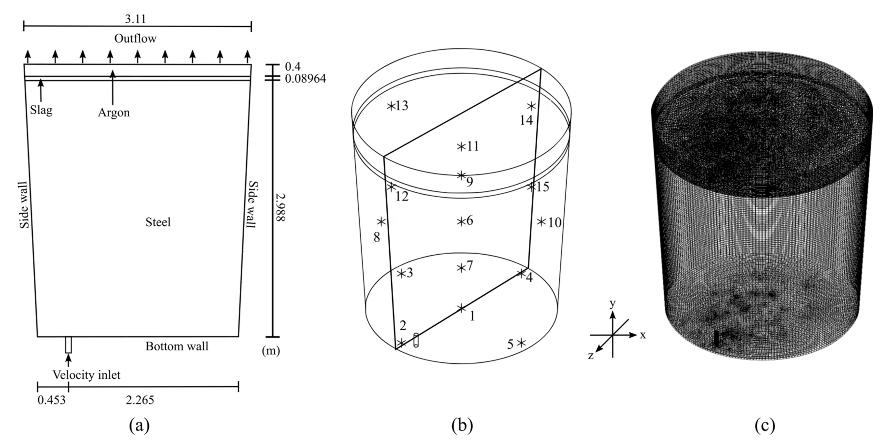
2.2.1. Boundary Conditions and Material Properties

For the simulation of the industrial process, a 140-t ladle furnace stirred by an argon gas bottom for a time of 15 min was considered. Gas flow rates of 0.3, 0.45, and 0.5 Nm³·min⁻¹ were injected. For the numerical simulation, the following considerations were taken into account: the calculations were developed in a transitory state, the injected gas flow was constant, the walls had a non-slip condition, the gravitational acceleration was exerted only in the negative direction of the y-axis, the bath temperature was homogeneous at the start of the simulation, and the thickness of the slag layer was uniform at the beginning of the calculations.

Table 1. Material properties and parameters used in numerical simulation.

Material	Density (kg·m−3)	Viscosity (kg·m−1·s−1)	Surface Tension (N·m−1)	Heat Capacity (J·kg−1·K−1)	Thermal Conductivity (W·m−1·K−1)
Water	998.2 [14]	0.001003 [14]	-	-	-
Oil	871	0.027872	-	-	-
Air	1.227	1.7 × 10−5	-	-	-
Water-air	*	*	0.072	-	-
Water-oil	*	*	0.021	-	-
Oil-air	*	*	0.04	-	-
Steel	$8586-0.8567·T$ [5]	$0.3147\times {10}^{-03}{e}^{\left(\frac{46480}{8.314·T}\right)}$ [5]	-	$\begin{array}{l}452.963\\ +\left(176.704\times {10}^{-3}\right)T\\ -\left(482.082\times {10}^{-5}\right)T^{-2}\end{array}$ [5]	41 [14]
Slag	2800 [14]	${\mu }_{\mathrm{slag}}=f\left(T,\%\mathrm{wt}.\right)$ [31]	-	$\begin{array}{l}{\displaystyle \sum _{n=1}^j\left(C_p^{{\mathrm{MO}}_n}{X}_{{\mathrm{MO}}_n}\right)}\\ \mathrm{MO}=\mathrm{Slag} \mathrm{oxide}\end{array}$ [5]	0.48 [14]
Argon	1.6228 [14]	2.125 × 10−5 [14]	-	520.64 [14]	0.0158 [14]
Steel-slag	*	*	1.15 [14]	-	-
Steel-argon	*	*	1.82 [14]	-	-
Slag-argon	*	*	0.58 [14]	-	-

* Calculated by Equations (25) and (26).

shows the parameters and properties of the materials considered in the experimental and numerical techniques.

The viscosity of the slag is a function of temperature and composition, and, in this work, a slag composed of 55% CaO, 30% Al₂O₃, 7.5% MgO, 7.5% SiO₂ was used. The calculation of the viscosity, ${\mu }_{\mathrm{slag}}$, was performed using Equation (2) obtained from data reported in the literature [31]:

$${\mu }_{\mathrm{slag}}=144.6878212-0.147368·T+3.88\times {10}^{-5}·T^2$$

(2)

The dimensions of the ladle are shown in Figure 2a, as well as the boundary conditions and the distribution of the phases considered. For the analysis of the temperature into the steel during the simulation, 15 monitoring points were established, homogeneously distributed throughout the volume of the steel, and thus guaranteeing the global evolution of the temperature, as shown in Figure 2b. On the other hand,

Table 2. Spatial sensors location.

Sensor	Coordinates
	r (m)	z (m)	θ (°)
1	0	0	0
2	1.2	0	180
3	1.2	0	90
4	1.2	0	0
5	1.2	0	270
6	0	1.5	0
7	1.13	1.5	135
8	1.13	1.5	45
9	1.13	1.5	315
10	1.13	1.5	225
11	0	2.8	0
12	1.98	2.8	180
13	1.98	2.8	90
14	1.98	2.8	0
15	1.98	2.8	270

shows the position of each monitoring sensor in cylindrical coordinates. Figure 2c shows the employed mesh, and the sensitivity technique was chosen to optimize its refinement based on the axial velocity of the steel at the middle ladle height, as shown in Figure 3. According to the results, no differences between the mesh of 1,247,337 elements and that of 1,500,000 elements were found; the first being selected to perform the calculations and thus to reduce the computational cost. Two different heat fluxes were employed, which were associated with the two refractory types most used in the plant for metallurgical ladles, the Al₂O₃ and Mg-C heat fluxes of −6400 and −13,750 W·m⁻², respectively [14].

The solutions of the continuity, momentum, and energy equations were performed using the Eulerian multiphase model [32], included in the Ansys Fluent 15.0^® software (Ansys Inc., Canonsburg, PA, USA). This model solved the equations and performed the mass and energy balances using a pressure-based solver, considering a convergence criteria 1 × 10⁻⁴ for all variables. A Dell Precision T1700^® Intel Xeon E3-1241 v3–3.5 GHz, 16 GB RAM (Intel Corporation, Mountain View, CA, USA) was employed.

2.2.2. Continuity Equation

The mass conservation was established according to Equation (3) [32]:

$$\frac{\partial }{\partial t}\left({\alpha }_q{\rho }_q\right)+\nabla \cdot ({\alpha }_q{\rho }_q{\overrightarrow{v}}_q)=0$$

(3)

where ${\alpha }_q$, ${\rho }_q$, and ${\overrightarrow{v}}_q$ are volume fraction; density, kg·m⁻³; and velocity, m·s⁻¹; for phase q, respectively.

2.2.3. Momentum Equation

The force balance in system was solved by Equation (4) [32]:

$$\frac{\partial }{\partial t}\left({\alpha }_q{\rho }_q{\overrightarrow{v}}_q\right)+\nabla \cdot \left({\alpha }_q{\rho }_q{\overrightarrow{v}}_q{\overrightarrow{v}}_q\right)=-{\alpha }_q\nabla p+\nabla \cdot {\overline{\overline{\tau }}}_q+{\alpha }_q{\rho }_q\overrightarrow{g}+{\displaystyle \sum _{p=1}^n{\overrightarrow{R}}_{pq}}+\left({\overrightarrow{F}}_{lift,q}+{\overrightarrow{F}}_{td,q}\right)$$

(4)

Here, p is static pressure, Pa; $\rho \overrightarrow{g}$ is force due to gravitational acceleration, m·s⁻²; ${\overrightarrow{F}}_{lift,q}$ and ${\overrightarrow{F}}_{td,q}$ are lift force and turbulent dispersion force for phase q, respectively (in N); and ${\overrightarrow{R}}_{pq}$ is the interaction force between phases. The strain-stress tensor, ${\overline{\overline{\tau }}}_q$, is defined by Equation (5):

$${\overline{\overline{\tau }}}_q={\alpha }_q{\mu }_q\left(\nabla {\overrightarrow{v}}_q+\nabla {\overrightarrow{v}}_q^T\right)+{\alpha }_q\left({\lambda }_q-\frac{2}{3}{\mu }_q\right)\nabla \cdot {\overrightarrow{v}}_q\overline{\overline{I}}$$

(5)

where, ${\mu }_q$ and ${\lambda }_q$ are the shear and bulk viscosities for phase q, respectively [32].

2.2.4. k-$\epsilon$ Realizable Turbulence Model

Turbulence was modeled using the k-$\epsilon$ realizable model [33], and it is described by Equations (6) and (7):

$$\frac{\partial }{\partial t}\left(\rho \mathrm{k}\right)+\frac{\partial }{\partial x_j}\left(\rho \mathrm{k}{u}_j\right)=\frac{\partial }{\partial x_j}\left[\left(\mu +\frac{{\mu }_t}{{\sigma }_{\mathrm{k}}}\right)\frac{\partial \mathrm{k}}{\partial x_j}\right]+G_{\mathrm{k}}+G_b-\rho \epsilon$$

(6)

$$\frac{\partial }{\partial t}\left(\rho \epsilon \right)+\frac{\partial }{\partial x_j}\left(\rho \epsilon u_j\right)=\frac{\partial }{\partial x_j}\left[\left(\mu +\frac{{\mu }_t}{{\sigma }_{\epsilon }}\right)\frac{\partial \epsilon }{\partial x_j}\right]+\rho C_{1}S\epsilon -\rho C_2\frac{{\epsilon }^2}{\mathrm{k}+\sqrt{v\epsilon }}$$

(7)

where, k and $\epsilon$ are kinetic turbulent energy, J·kg⁻¹, and the turbulent dissipation rate, m²·s⁻³, respectively. ${\mu }_t$ is the turbulent viscosity, m²·s⁻¹. ${\sigma }_{\mathrm{k}}$ and ${\sigma }_{\epsilon }$ are the Prandtl number for k and $\epsilon$ whose values are 1.0 and 1.2, respectively [33]. $G_{\mathrm{k}}$ and $G_b$ represent the generation of turbulence kinetic energy due to the mean velocity gradients and buoyancy, respectively. $C_{1\epsilon }$ and $C_2$ are constants, and their corresponding values are 1.44 and 1.9 [33]. $C_1$ was calculated according to Equations (8)–(10):

$$C_1=\max \left[0.43,\frac{\eta }{\eta +5}\right]\mathrm{c}$$

(8)

$$\eta =S\frac{\mathrm{k}}{\epsilon }$$

(9)

$$S=\sqrt{2S_{ij}{S}_{ij}}$$

(10)

Turbulent viscosity was determined by Equation (11):

$${\mu }_t=\rho C_{\mu }\frac{{\mathrm{k}}^2}{\epsilon }$$

(11)

$C_{\mu }$ was calculated using Equations (12)–(19):

$$C_{\mu }=\frac{1}{A_0+A_s\frac{\mathrm{k}{U}^{*}}{\epsilon }}; A_0=4.04, A_s=\sqrt{6}\cos \varphi$$

(12)

$$\cos \varphi =\frac{1}{3}{\cos }^{-1}\left(\sqrt{6}W\right)$$

(13)

$$W=\frac{S_{ij}{S}_{jk}{S}_{ki}}{{\tilde{S}}^3}$$

(14)

$$\tilde{S}=\sqrt{S_{ij}{S}_{ij}}\tilde{S}$$

(15)

$$S_{ij}=\frac{1}{2}\left(\frac{\partial u_j}{\partial x_i}+\frac{\partial u_i}{\partial x_j}\right)$$

(16)

$$U*\equiv \sqrt{S_{ij}{S}_{ij}+{\tilde{\mathsf{\Omega }}}_{ij}{\tilde{\mathsf{\Omega }}}_{ij}}$$

(17)

$${\tilde{\mathsf{\Omega }}}_{ij}={\mathsf{\Omega }}_{ij}-2{\epsilon }_{ijk}{\omega }_k$$

(18)

$${\mathsf{\Omega }}_{ij}=\overline{{\mathsf{\Omega }}_{ij}}-{\epsilon }_{ijk}{\omega }_k$$

(19)

Here, $u$ represents the mean velocity component. $S$ is a scalar measure of the deformation tensor. $\overline{{\mathsf{\Omega }}_{ij}}$ is the mean rate-of-rotation tensor along the moving reference frame, and ${\omega }_k$ represents angular velocity.

2.2.5. Troshko–Hassan Turbulence Interaction

The influence of the disperse phase (argon and slag) on the turbulence equations was modeled using the Troshko–Hassan model [34]. For continuous phase q, the source terms were calculated by Equations (20) and (21):

$${\prod }_{k_q}=C_{\mathrm{k}e}{\displaystyle \sum _{p=1}^M\frac{K_{pq}}{{\alpha }_q{\rho }_q}{\left|{\overrightarrow{U}}_p-{\overrightarrow{U}}_q\right|}^2}$$

(20)

$${\prod }_{{\epsilon }_q}=C_{td}\frac{1}{{\tau }_p}{\prod }_{k_q}$$

(21)

where, $\overrightarrow{U}$ is the phase-weighted velocity of the phase; $C_{\mathrm{k}e}$ and $C_{td}$ are constants whose values are 0.75 and 0.45, respectively; and the term $K_{pq}$ is the interphase momentum exchange coefficient, and it is related with the momentum equation (Equation (4)) according to Equation (22):

$${\displaystyle \sum _{p=1}^n{\overrightarrow{R}}_{pq}}={\displaystyle \sum _{p=1}^n{K}_{pq}\left({\overrightarrow{v}}_p-{\overrightarrow{v}}_q\right)}$$

(22)

${\overrightarrow{v}}_p$ and ${\overrightarrow{v}}_q$ are the velocities of each phase, and ${\tau }_p$ is the characteristic time of induced turbulence defined by Equation (23):

$${\tau }_p=\frac{2C_{VM}{d}_p}{3C_D\left|{\overrightarrow{U}}_p-{\overrightarrow{U}}_q\right|}$$

(23)

Here, $C_{VM}$ is the virtual mass coefficient, and $C_D$ represents the drag coefficient. To calculate the kinematic turbulent viscosity ($\nu$) of the dispersed phase, Equation (24) is used:

$${\nu }_p={\nu }_q$$

(24)

2.2.6. Symmetric Drag Model

To determine the interphase momentum exchange coefficient, $K_{pq}$, the symmetric model was employed [32]. This model uses Equations (25) and (26) to calculate properties such as density and viscosity:

$${\rho }_{pq}={\alpha }_p{\rho }_p+{\alpha }_q{\rho }_q$$

(25)

$${\mu }_{pq}={\alpha }_p{\mu }_p+{\alpha }_q{\mu }_q$$

(26)

Particle diameter was determinate, using the diameters of phase q and p, by Equation (27):

$$d_{pq}=\frac{1}{2}\left(d_p+d_q\right)$$

(27)

$K_{pq}$ was calculated by Equations (28)–(31):

$$K_{pq}=\frac{{\rho }_{pq}f}{6{{\tau }^{\prime }}_{pq}}{d}_p{A}_i$$

(28)

$${{\tau }^{\prime }}_{pq}=\frac{{\rho }_{pq}{\left(d_{pq}\right)}^2}{18{\mu }_{pq}}$$

(29)

$$f=\frac{C_D\mathrm{Re}}{24}$$

(30)

$$\mathrm{Re}=\frac{{\rho }_{pq}\left|{\nu }_p-{\nu }_q\right|d_{pq}}{{\mu }_{pq}}$$

(31)

Here, Re expresses the dimensionless Reynolds number. $A_i$ is the interfacial area, m²; f is the drag function, and it is calculated according to the criteria described in Equation (32) [33]:

$$C_D=\left\{\begin{array}{l}\frac{24}{\mathrm{Re}}\left(1+0.15{\mathrm{Re}}^{0.687}\right)\Rightarrow \mathrm{Re}\le 1000\\ 0.44\Rightarrow \mathrm{Re}>1000\end{array}\right.$$

(32)

2.2.7. Lift Model

The lift effect was included using the Tomiyama lift model [29]. According to the model, the lift force can be determined by Equation (33):

$${\overrightarrow{F}}_{lift}=-C_l{\rho }_q{\alpha }_p\left({\overrightarrow{v}}_q-{\overrightarrow{v}}_p\right)\times \left(\nabla \times {\overrightarrow{v}}_q\right)$$

(33)

where, $C_l$ is the lift coefficient, which is calculated according to Equations (34)–(38):

$$C_l=\left\{\begin{array}{l}\min \left[0.288\tanh \left(0.121{\mathrm{Re}}_p\right),f\left(E{o}^{\prime }\right)\right]E{o}^{\prime }\le 4\\ f\left(E{o}^{\prime }\right)4<E{o}^{\prime }\le 10\\ -0.2710<E{o}^{\prime }\end{array}\right.$$

(34)

$$f\left(E{o}^{\prime }\right)=0.00105E{o^{\prime }}^3-0.0159E{o^{\prime }}^2-0.0204E{o}^{\prime }+0.474$$

(35)

$$E{o}^{\prime }=\frac{g\left({\rho }_q-{\rho }_p\right)d_h^2}{\sigma }$$

(36)

$$d_h=d_b{\left(1+0.163E{o}^{0.757}\right)}^{0.333}$$

(37)

$$Eo=\frac{g\left({\rho }_q-{\rho }_p\right)d_b^2}{\sigma }$$

(38)

$Eo$ represents the dimensionless Eötvös number; this number relates buoyancy and surface tension forces. $E{o}^{\prime }$ is a modified Eötvös number, and it is based on the longer axis of the bubble, $d_h$. $\sigma$ is surface tension, N·m⁻¹; g is gravity acceleration, m·s⁻²; and $d_b$ is bubble diameter, m.

2.2.8. Virtual Mass

The virtual mass force exerted on a rising bubble is calculated by Equation (39) [35]:

$${\overrightarrow{F}}_{VM}=0.5{\alpha }_p{\rho }_p\left(\frac{d_q{\overrightarrow{v}}_q}{dt}-\frac{d_p{\overrightarrow{v}}_p}{dt}\right)$$

(39)

where, the phase material time derivative is formulated as Equation (40):

$$\frac{d_q\left(\varphi \right)}{dt}=\frac{\partial \left(\varphi \right)}{\partial t}+\left({\overrightarrow{v}}_q·\nabla \right)\varphi$$

(40)

2.2.9. Turbulent Dispersion Force

The force due to the turbulent dispersion effect was modeled using Burns et al.’s model [36]. Here, the dispersion scalar, $D_{tq}$, was calculated with Equation (41):

$$D_q=D_p=D_{tq}=\frac{{\mu }_{tq}}{{\rho }_q}$$

(41)

where, $D_q$ and $D_p$ are the scalar dispersion of the continuous and the disperse phase, respectively. Thus, the turbulent dispersion force was determined by Equation (42):

$${\overrightarrow{F}}_{td,q}=-{\overrightarrow{F}}_{td,p}=C_{TD}{K}_{pq}\frac{D_q}{{\sigma }_{pq}}\left(\frac{\nabla {\alpha }_p}{{\alpha }_p}-\frac{\nabla {\alpha }_q}{{\alpha }_q}\right)$$

(42)

where, ${\sigma }_{pq}$ is the dispersion Prandtl number, and its value is 0.9; the $C_{TD}$ constant value was set to 1 [36].

2.2.10. Energy Conservation

The energy equation from the Eulerian multiphase model is described by Equation (43) [33]:

$$\frac{\partial }{\partial t}\left({\alpha }_q{\rho }_q{h}_q\right)+\nabla \cdot \left({\alpha }_q{\rho }_q{h}_q{\overrightarrow{u}}_q\right)={\alpha }_q\frac{\partial p_q}{\partial t}+\overline{\overline{\tau }}:\nabla {\overrightarrow{u}}_q-\nabla \cdot {\overrightarrow{q}}_q+{\displaystyle \sum _{p=1}^n\left(Q_{pq}\right)}$$

(43)

where, $h_q$ is the specific enthalpy for phase q; ${\overrightarrow{q}}_q$ is the heat flux, W·m⁻²; and $Q_{pq}$ represents the intensity of the heat exchange between phases.

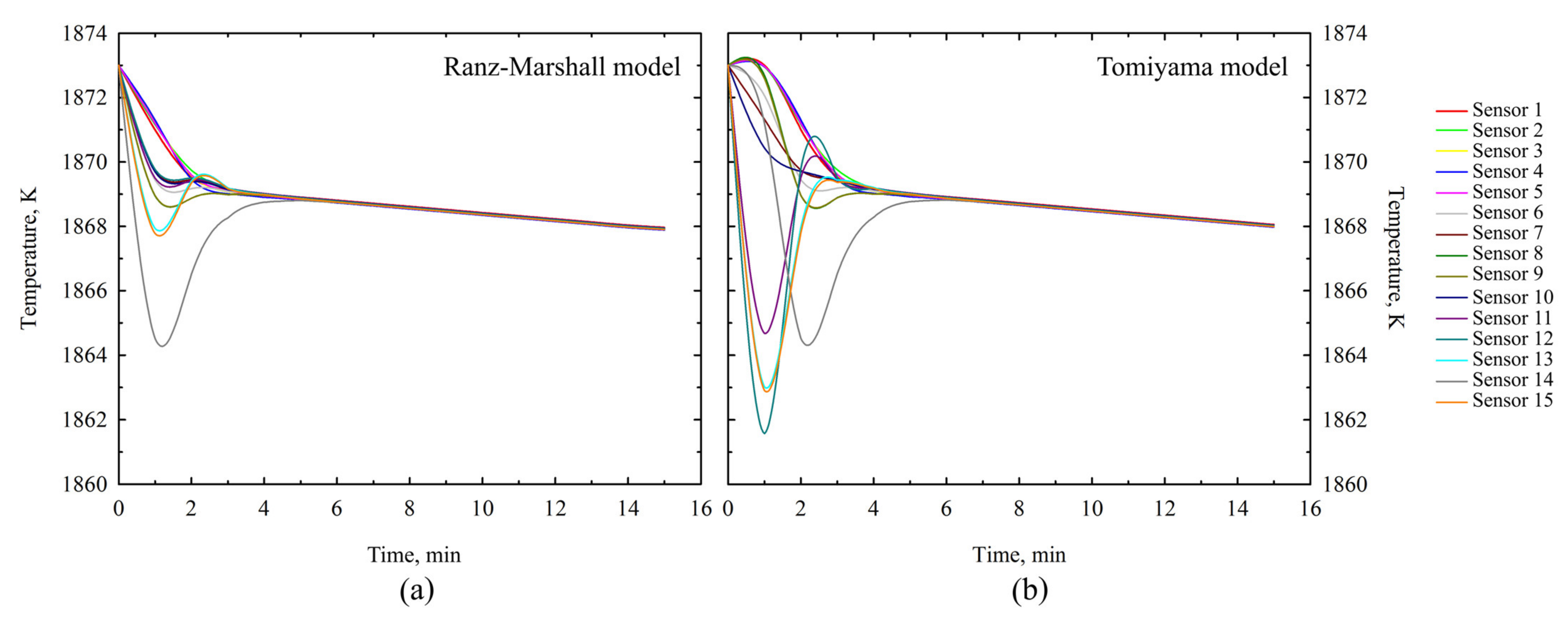
2.2.11. Heat Exchange Coefficient

The volumetric energy transfer rate between phases, $Q_{pq}$, in W is defined by Equation (44) [33]:

$$Q_{pq}=h_{pq}{A}_i\left(T_p-T_q\right)$$

(44)

where, $h_{pq}$ is the volumetric heat transfer coefficient between phases p and q; $A_i$ represents the interfacial area, m²; and $T_p$ and $T_q$ are phases p and q in K, respectively.

The volumetric heat transfer coefficient was calculated from the Nusselt number, Nu, using Equation (45) [33]:

$$h_{pq}=\frac{{\kappa }_q{\mathrm{Nu}}_p}{d_p}$$

(45)

where,${\kappa }_q$ is the thermal conductivity of phase q, W·m⁻¹·K⁻¹, and $d_p$ is the bubble diameter, m.

There are several models to determine $h_{pq}$; however, two models were considered in this study. The Ranz–Marshall model [28] proposes Equation (46) to calculate the Nusselt number:

$${\mathrm{Nu}}_p=2.0+0.6{\mathrm{Re}}_p^{0.5}{\mathrm{Pr}}^{0.33}$$

(46)

Here, Re and Pr are the Reynolds and Prandtl dimensionless numbers, respectively. The Prandtl number was computed according to Equation (47):

$$\mathrm{Pr}=\frac{C_{p_q}{\mu }_q}{{\kappa }_q}$$

(47)

where, $C_{p_q}$ is the heat capacity of phase q, J·kg⁻¹·K⁻¹.

Alternatively, the Tomiyama model [29] calculates the Nusselt number by Equation (48):

$${\mathrm{Nu}}_p=2.0+0.15{\mathrm{Re}}_p^{0.8}{\mathrm{Pr}}^{0.5}$$

(48)

2.2.12. Discrete Ordinates Radiation Model

The discrete ordinates radiation model [37,38,39] was employed to solve the radiation equation. This model uses a finite number of discrete solid angles associated to the vector direction, and it is described by Equation (49):

$$\nabla \cdot \left(I\left(\overrightarrow{r},\overrightarrow{s}\right)\overrightarrow{s}\right)+\left(a+{\sigma }_s\right)I\left(\overrightarrow{r},\overrightarrow{s}\right)=a{n}^2\frac{\sigma T^4}{\pi }+\frac{{\sigma }_s}{4\pi }{\displaystyle \underset{0}{\overset{4\pi }{\int }}I\left(\overrightarrow{r},{\overrightarrow{s}}^{\prime }\right)}\mathrm{\Phi }\left(\overrightarrow{s},{\overrightarrow{s}}^{\prime }\right)d{\mathsf{\Omega }}^{\prime }$$

(49)

It is applicable for an emitting, absorbing, and scattering medium. $\overrightarrow{r}$, $\overrightarrow{s}$, and ${\overrightarrow{s}}^{\prime }$ are the position, direction, and scattering direction vector, respectively. s, n, and a represent the path length, the refractive index, and the absorption coefficient (0.9 and 0.83 for steel and slag, respectively). ${\sigma }_s$ is the scattering coefficient, and $\sigma$ is the Stefan–Boltzmann constant, 5.669 × 10⁻⁸ W·m⁻²·K⁻⁴. The radiation intensity and the local temperature are defined by I and T, respectively. $\mathrm{\Phi }$ is a phase function, and ${\mathsf{\Omega }}^{\prime }$ is the solid angle. The emissivity was set as 0.3 [40].

3. Results and Discussion

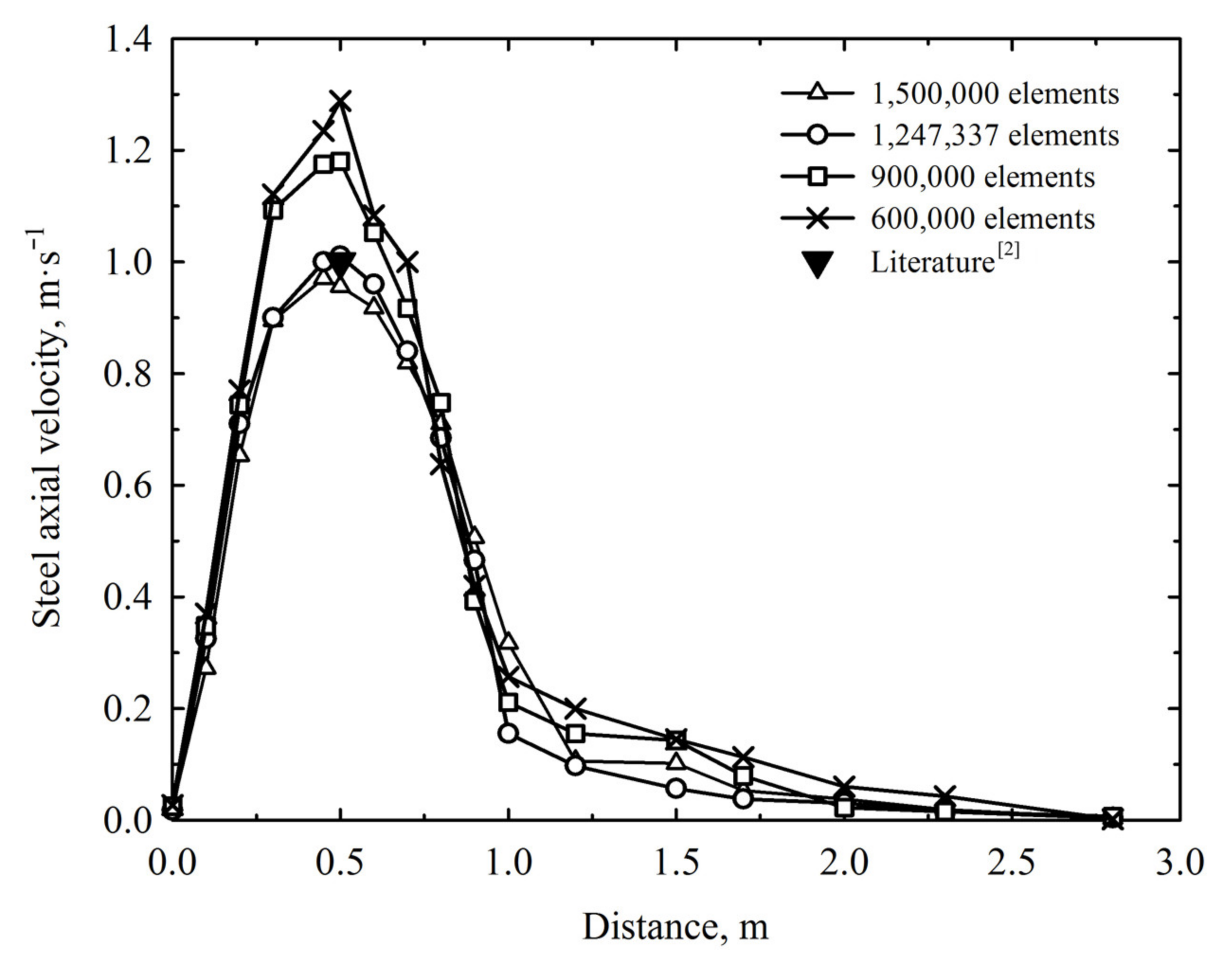
3.1. Fluid Dynamics Validation

For the validation, the results of velocity magnitude and slag layer opening obtained by numerical simulation were compared with those obtained by the PIV technique, as shown in Figure 4a,b, respectively. The effects of all drag and non-drag forces were included in the simulation according to the conclusions established in previous studies [6,41]. The highest velocity was reached in the plume region because of the rising air bubbles. The transfer of the momentum between the bubbles and the water produced a movement of the liquid from the bottom towards the free surface, producing a recirculation pattern as observed in points ① and ❶. The location of the recirculation pattern and the magnitudes of the water velocities predicted adequately fit those obtained experimentally. Figure 4c,d compares the openings of the oil layer at the same experimental and numerical calculation time, ~15 s. The opening was primarily located in the region of the broken free surface by the plume; however, the convective movement and momentum exchange at the interface prolonged the opening beyond the spout. It was observed that the shape of the oil aperture was very similar in both cases, and an oil aperture difference of ~3.7% was determined using the ImageJ^® analyzer software (National Institutes of Health, Bethesda, MD, USA).

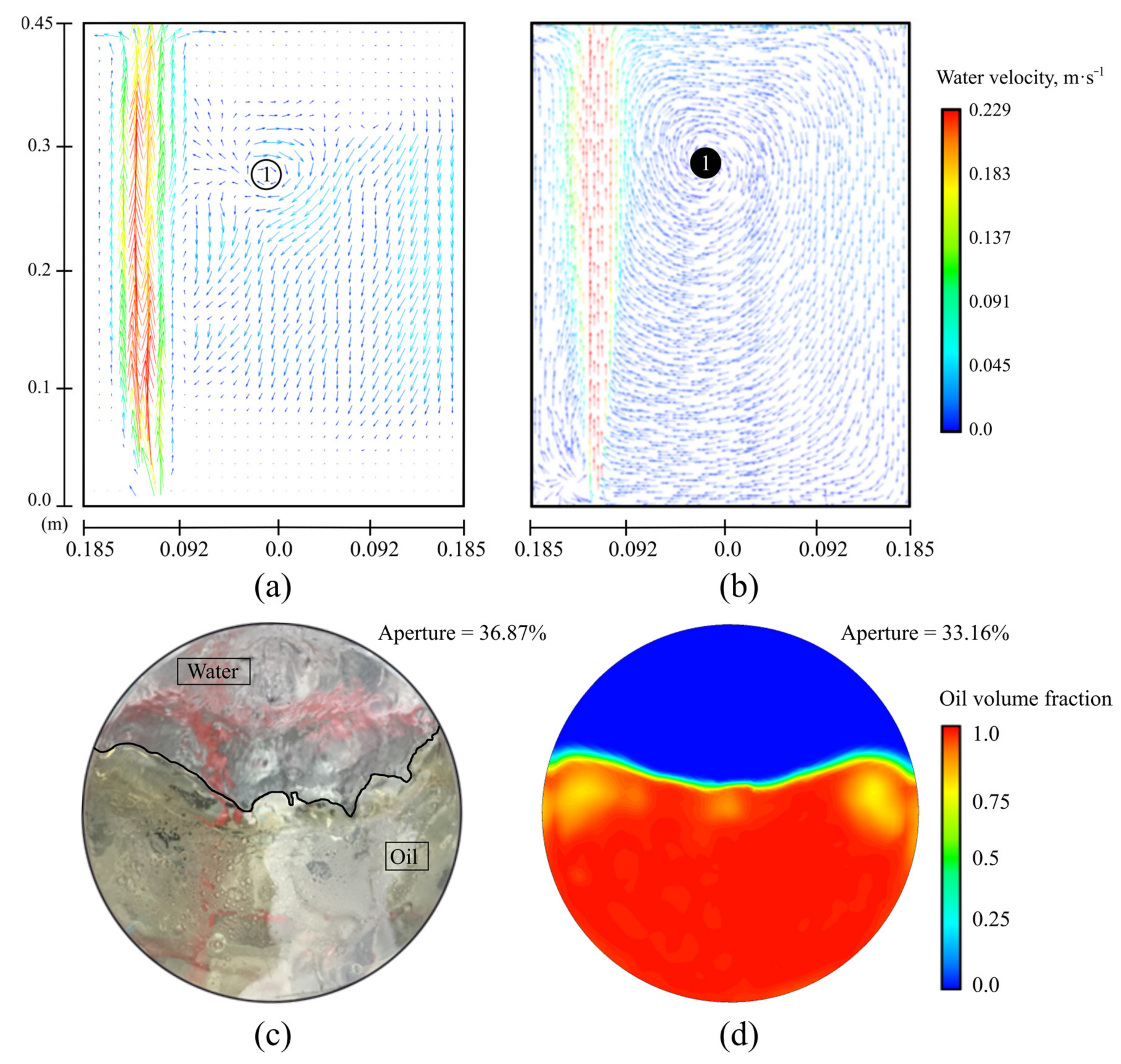
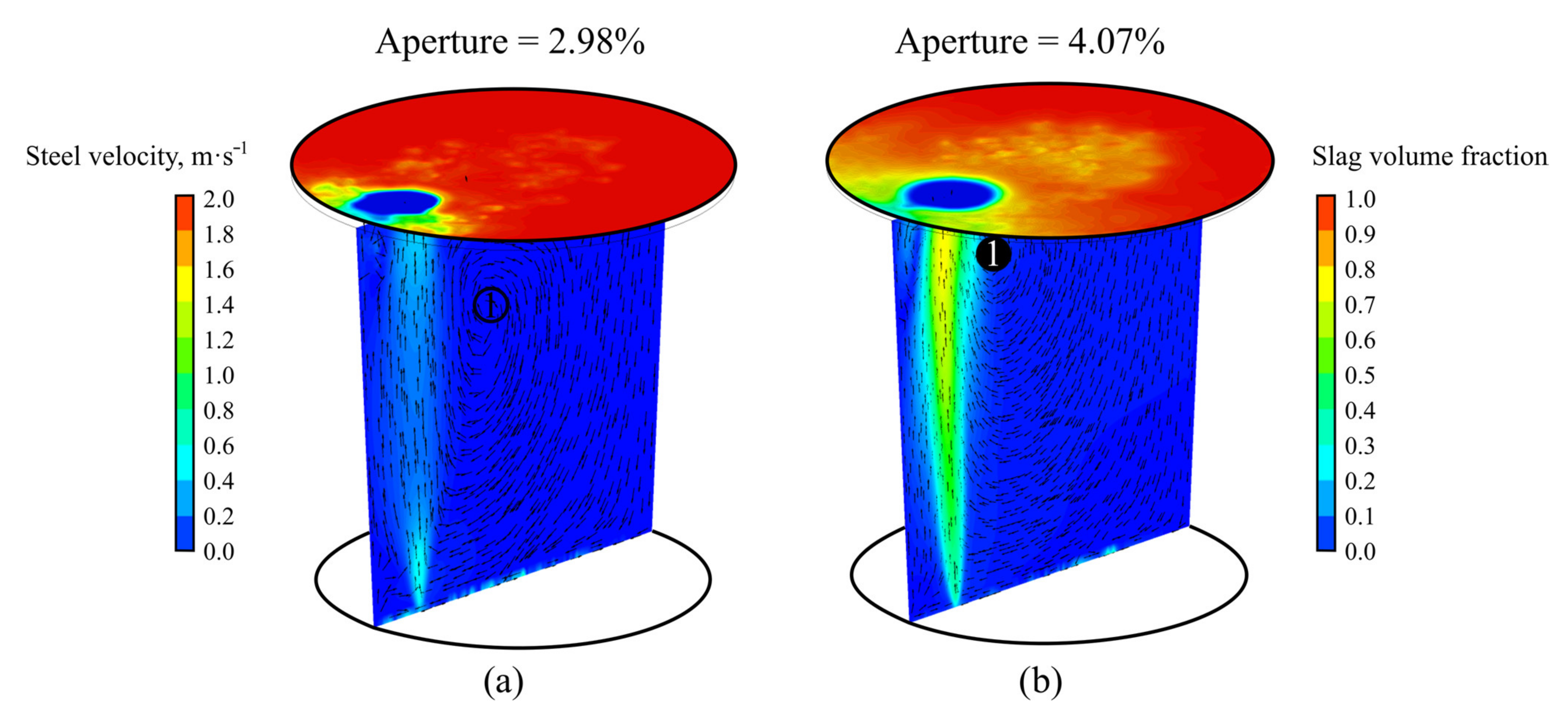
3.2. Behavior of the Gas Flow Rate and the Slag Eye Aperture

The effect of the injected argon flow, 0.3 and 0.5 Nm³·min⁻¹, on the fluid dynamics structure of the steel is shown in Figure 5 for the industrial ladle. The velocity of the plume was slow using the gas flow of 0.3 Nm³·min⁻¹ because of the ferrostatic pressure exerted by the steel that delayed the ascending gas plume (Figure 5a). In both cases, there was the formation of a recirculation pattern, but it was located in different positions. With low injection, the momentum was less, and the drag effect was increased, causing a recirculation in the middle of the ladle at point ①. With a flow of 0.5 Nm³·min⁻¹ (Figure 5b), the recirculation position was located close to the free surface caused by a higher momentum exchange between argon and steel, point ❶. The injected gas flow influenced the shape and size of the opening slag eye. A flow of 0.3 Nm³·min⁻¹ (Figure 5a) had a slightly smaller opening than when using a high gas flow (Figure 5b). This difference was attributed to a lower impact force at the steel-slag interface, which led to a reduction in slag displacement. The quantitative difference of the aperture areas was ~1.1% and was similar to that reported in the literature [14].

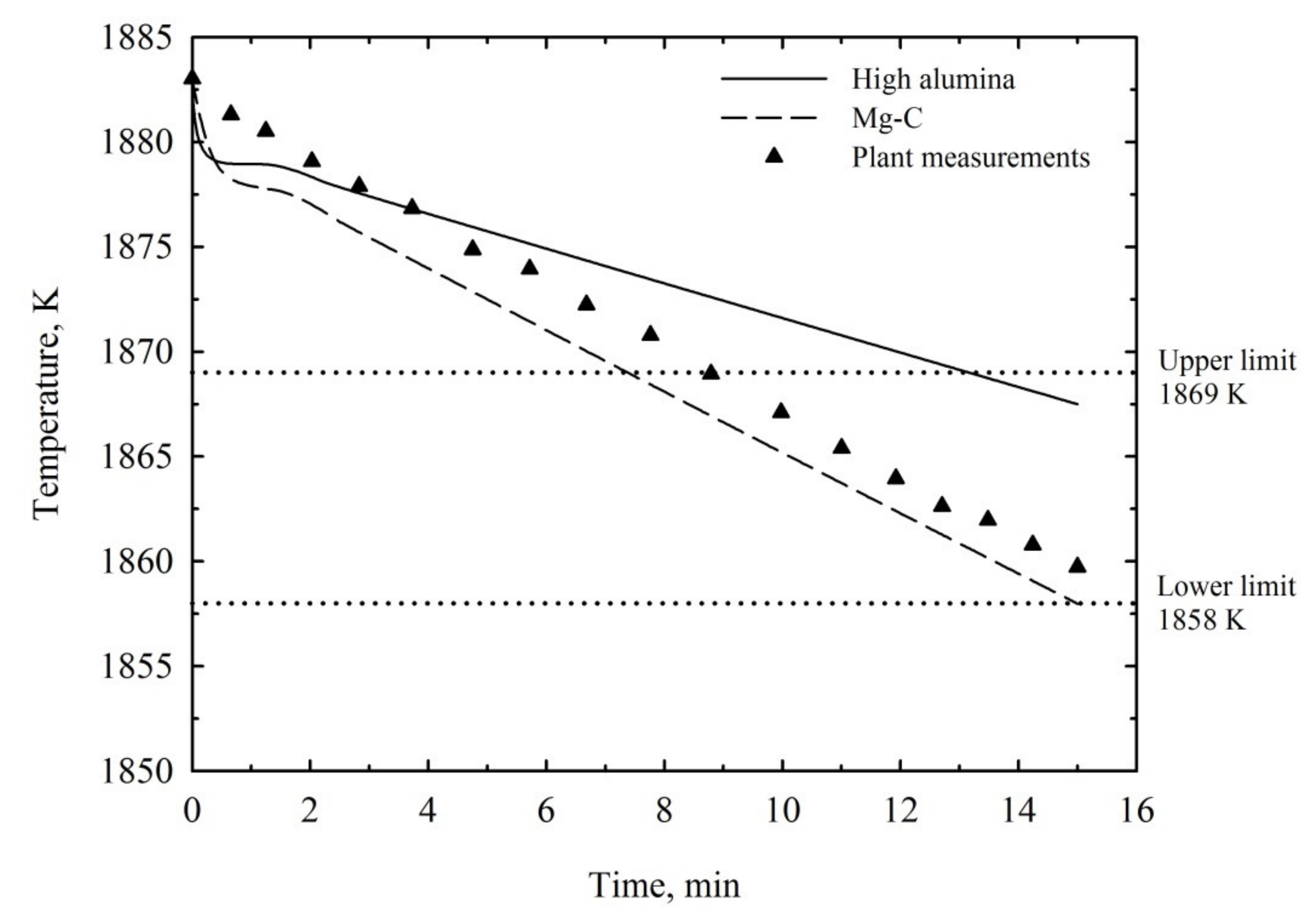
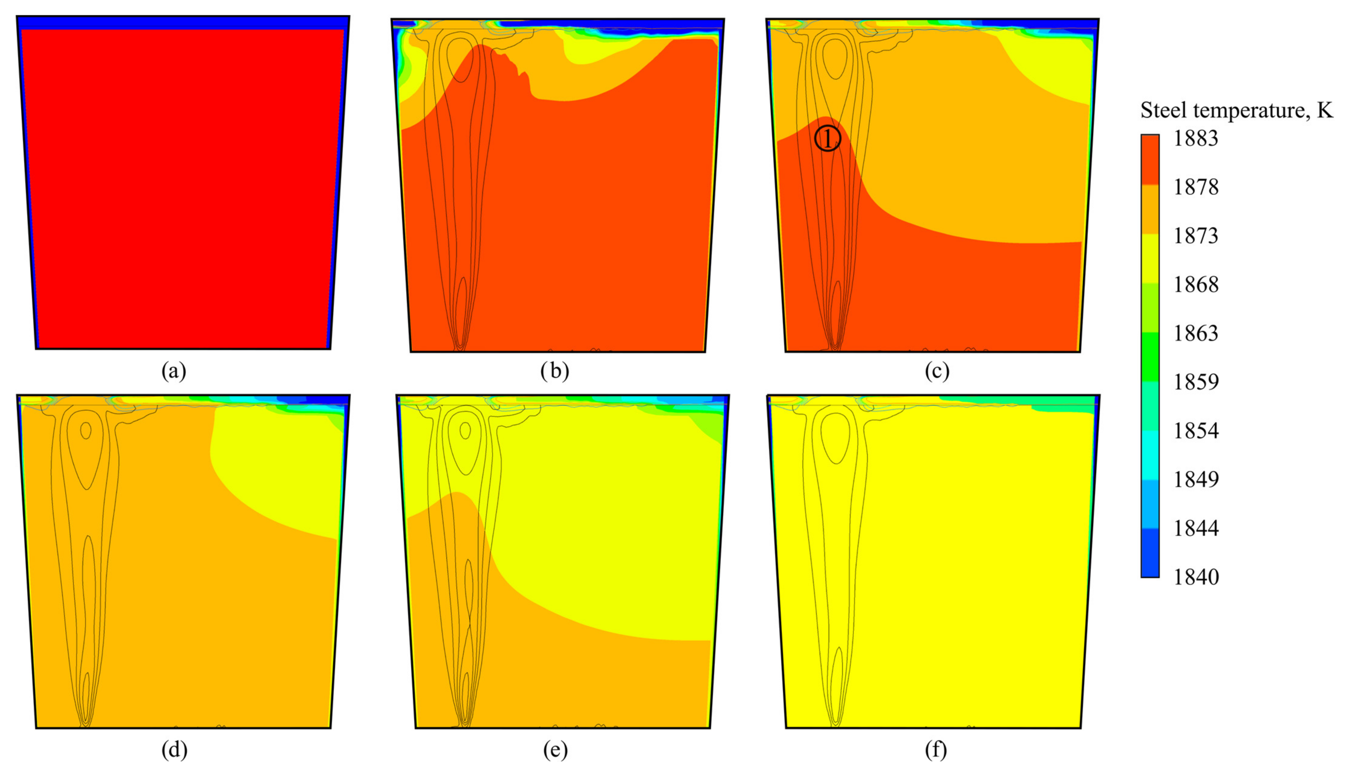
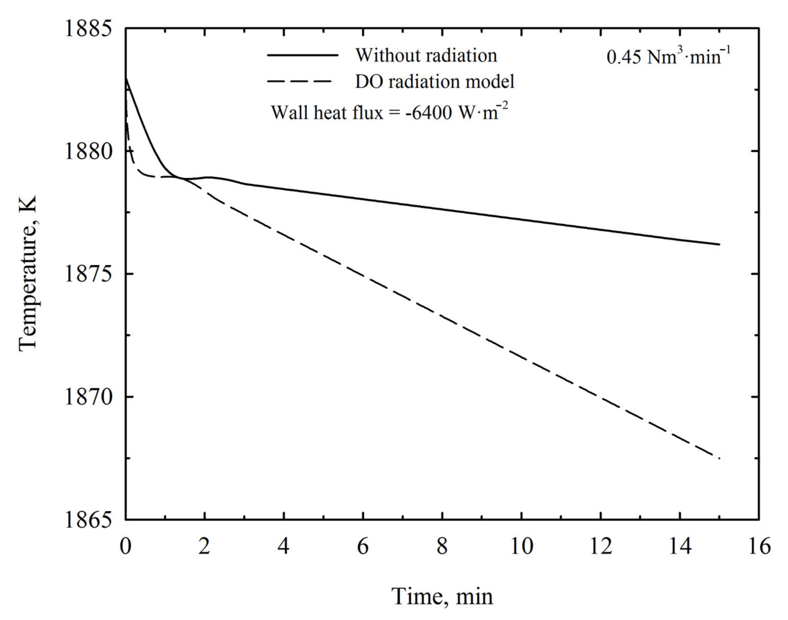
3.3. Thermal Behavior of Steel in the Ladle

The Ranz–Marshall model [28] has been used to calculate the thermal behavior of steel in a satisfactory way [11]; however, in this work, the models of Ranz-Marshall and Tomiyama [29] were compared. The latter was used because it was used in the solution for the lift forces in the fluid dynamics calculation. Figure 6 shows the steel temperature predicted by the Ranz-Marshall and Tomiyama models in a 15 min process period. The injected gas flow was 0.45 Nm³·min⁻¹, and a boundary condition of heat loss through the walls of −6400 W·m² was used, omitting the radiation mechanism for this case. During the first 5 min, there was no homogeneity in the temperature of the steel because of the transfer of heat in the plume and the walls. However, after 5 min, the temperature was the same in all the sensors, and they dropped to a temperature of approximately 1868 K. This final temperature did not show significant differences between the models since both reached a value of 1868 K.

In the industrial process, the usage of argon gas generates the opening of the slag layer, causing the steel to be exposed to the atmosphere, favoring the transfer of heat through the radiation mechanism according to Farrera et al. [14]. This is shown in Figure 7, where the effect of the incorporation of the radiation model is compared. The numerical calculation using the DO model yielded a difference of 9 K in the final temperature of the steel when it was not used. The initial drop in temperature at 30 s was more pronounced when the DO model was used because of the removal of heat by the free surface, and, subsequently, it descended at a constant rate. The foregoing demonstrates the importance of incorporating a radiation model for the analysis of the thermal behavior of steel in a secondary refining ladle.

Figure 8 compares the results obtained by the mathematical model using the Tomiyama model and the DO model. Two different boundary conditions were considered across the walls for heat extraction, associated with Mg-C and high alumina refractories with values of −13,750 W·m⁻² and −6400 W·m⁻², respectively, and an initial steel temperature of 1883 K. The results using the Mg-C refractory showed a final temperature of 1867 K after 15 min of stirring, with a slope of 1.66 K·min⁻¹, whereas the high alumina refractory produced a less intense cooling rate with a slope of 1.06 K·min⁻¹. Figure 8 also shows the comparison of the plant data [14] with the results obtained in the mathematical model under the same conditions with the Mg-C refractory. In this, it can be seen that the temperature difference at the end of the calculation time was only 1 K and that both slopes are similar, allowing the model to be used with confidence to predict the thermal evolution of the steel. In the industry, a final temperature range of the steel is recommended (delimited by the dotted lines), and both numerical models using different refractory materials are kept within the range.

The temperature contours of the thermal evolution of the steel using an injection flux of 0.45 Nm³·min⁻¹ are shown in Figure 9. Initially, the temperature of the steel was at 1883 K according to the initial condition (Figure 9a). At 30 s (Figure 9b), the effect of radiation caused a decrease in temperature near the free surface of the steel. At 1 min (Figure 9c), the steel remained hotter in the lower zone of the ladle, showing a drop in temperature as it approached the free surface. The influence of the plume was also noticeable when modifying the contour in the upward zone, as indicated in point ①. At 1.5 and 2 min—represented by Figure 9d,e, respectively—temperature gradients were significantly reduced, reaching the total thermal homogenization of the steel at 2.5 min, as shown in Figure 9f. This thermal homogenization time was similar to that reported by Castillejos et al. [27] where they established that convective mechanisms are dominant in the homogenization of temperature. However, they did not include the effect of free surface radiation, and the correspondence in this homogenization time was due to the fact that the authors [27] employed a greater through-wall cooling rate of −12,500 W·m⁻².

4. Conclusions

In this work, the fluid dynamics and thermal evolution of a multiphase system were studied using the Eulerian model with drag and non-drag forces and the Ranz-Marshall, Tomiyama, and DO models during the gas stirring process in the ladle furnace. According to the results, the following conclusions were drawn:

• The selected multiphase models correctly predicted the fluid dynamics of a three-phase system (water-oil-air). The velocity of the water and the shape and area of the opening of the oil layer predicted mathematically had good agreement with the experimental data, through the PIV technique.
• It was observed that there were no significant differences between the results calculated for the coefficients of heat exchange between the Ranz-Mạrshall and Tomiyama models. However, the Tomiyama model was chosen because of its affinity with the lift model for fluid dynamics simulation.
• Despite both refractories retaining enough heat to keep the steel temperature within industrial limits, the Al₂O₃ one had better heat retention, which would favor refining operations. However, for the desulfurization process, the use of basic refractories such as Mg-C is recommended to favor the reactions involved, and the operational cost is lower.
• The inclusion of the radiation mechanism contributes to the precision of the simulation of the thermal evolution of the steel into the ladle furnace. The DO radiation model correctly predicted heat loss through the free surface, reaching steel thermal homogenization at 2.5 min.

References

1. Cao, Q.; Pitts, A.; Nastac, L. Numerical modelling of fluid flow and desulphurisation kinetics in an argon-stirred ladle furnace. Ironmak. Steelmak. 2016, 45, 280–287. [Google Scholar] [CrossRef]
2. Singh, U.; Anapagaddi, R.; Mangal, S.; Padmanabhan, K.A.; Singh, A.K. Multiphase modeling of bottom-stirred ladle for prediction of slag–steel interface and estimation of desulfurization behavior. Metall. Mater. Trans. B 2016, 47, 1804–1816. [Google Scholar] [CrossRef]
3. Liu, Z.; Li, L.; Li, B. Modeling of gas-steel-slag three phase flow in ladle metallurgy: Part, I. Physical modeling. ISIJ Int. 2017, 57, 1971–1979. [Google Scholar] [CrossRef] [Green Version]
4. Li, L.; Li, B.; Liu, Z. Modeling of gas-steel-slag three phase flow in ladle metallurgy: Part II. Multi-scale Mathematical model. ISIJ Int. 2017, 57, 1980–1989. [Google Scholar]
5. Jonsson, L.; Jönsson, P. Modeling of fluid flow conditions around the slag/metal interface in a gas-stirred ladle. ISIJ Int. 1996, 36, 1127–1134. [Google Scholar] [CrossRef] [Green Version]
6. Lou, W.; Zhu, M. Numerical simulation of gas and liquid two-phase flow in gas-stirred systems based on euler–euler approach. Metall. Mater. Trans. B 2013, 44, 1251–1263. [Google Scholar] [CrossRef]
7. Villela-Aguilar, J.J.; Ramos-Banderas, J.A.; Hernández-Bocanegra, C.A.; Urióstegui-Hernández, A.; Solorio-Díaz, G. Optimization of the mixing time using asymmetrical arrays in both gas flow and injection positions in a dual-plug ladle. ISIJ Int. 2020, 60, 1172–1178. [Google Scholar] [CrossRef] [Green Version]
8. Senguttuvan, A.; Irons, G.A. Modeling of slag entrainment and interfacial mass transfer in gas stirred ladles. ISIJ Int. 2017, 57, 1962–1970. [Google Scholar] [CrossRef] [Green Version]
9. Cao, Q.; Nastac, L. Mathematical investigation of fluid flow, mass transfer, and slag-steel interfacial behavior in gas-stirred ladles. Metall. Mater. Trans. B 2018, 49, 1138–1404. [Google Scholar] [CrossRef] [Green Version]
10. Jönsson, P.; Jonsson, T. The use of fundamental process models in studying ladle refining operations. ISIJ Int. 2001, 41, 1289–1302. [Google Scholar] [CrossRef] [Green Version]
11. Xia, J.L.; Ahokainen, T. Homogenization of temperature field in a steelmaking ladle with gas injection. Scand. J. Metall. 2003, 32, 211–217. [Google Scholar] [CrossRef]
12. Mohammadi, D.; Seyedein, S.; Aboutalebi, M. Numerical simulation of thermal stratification and destratification in secondary steelmaking ladle. Ironmak. Steelmak. 2013, 40, 342–349. [Google Scholar] [CrossRef]
13. GOSH. Secondary Steelmaking Principles and Applications; CRC Press: Boca Raton, FL, USA, 2000. [Google Scholar]
14. Farrera-Buenrostro, J.E.; Hernández-Bocanegra, C.A.; Ramos-Banderas, J.A.; Torres-Alonso, E.; López-Granados, N.M.; Ramírez-Argáez, M.A. Analysis of temperature losses of the liquid steel in a ladle furnace during desulfurization stage. Trans. Indian Inst. Met. 2019, 72, 899–909. [Google Scholar] [CrossRef]
15. Xia, J.L.; Ahokainen, T. Transient flow and heat transfer in a steelmaking ladle during the holding period. Metall. Mater. Trans. B 2001, 32, 733–741. [Google Scholar] [CrossRef]
16. Ganguly, S.; Chakraborty, S. Numerical investigation on role of bottom gas stirring in controlling thermal stratification in steel ladles. ISIJ Int. 2004, 44, 537–546. [Google Scholar] [CrossRef]
17. Gonzalez, H.; Ramos-Banderas, J.A.; Torres-Alonso, E.; Solorio-Diaz, G.; Hernández-Bocanegra, C.A. Multiphase modeling of fluid dynamic in ladle steel operations under non-isothermal conditions. J. Iron Steel Res. Int. 2017, 24, 888–900. [Google Scholar] [CrossRef]
18. Chen, Y.C.; Bao, Y.; Wang, M.; Zhao, L.; Peng, Z. A mathematical model for the dynamic desulfurization process of ultra-low-sulfur steel in the LF refining process. Metall. Res. Technol. 2014, 111, 37–43. [Google Scholar] [CrossRef]
19. Volkova, O.; Janke, D. Modelling of temperature distribution in refractory ladle lining for steelmaking. ISIJ Int. 2003, 43, 1185–1190. [Google Scholar] [CrossRef]
20. Ilegbusi, O.; Szekely, J. Melt stratification in ladles. ISIJ Int. 1987, 27, 563–569. [Google Scholar] [CrossRef]
21. Grip, C.E.; Jonsson, L.; Jönsson, P.; Jonsson, K.O. Numerical prediction and experimental verification of thermal stratification during holding in pilot plant and production ladles. ISIJ Int. 1999, 39, 715–721. [Google Scholar] [CrossRef]
22. Pan, Y.; Björkman, B. Physical and mathematical modelling of thermal stratification phenomena in steel ladles. ISIJ Int. 2002, 42, 614–623. [Google Scholar] [CrossRef] [Green Version]
23. Pan, Y.; Grip, C.E.; Björkman, B. Numerical studies on the parameters influencing steel ladle heat loss rate, thermal stratification during holding and steel stream temperature during teeming. Scand. J. Metall. 2003, 32, 71–85. [Google Scholar] [CrossRef]
24. Austin, P.; Camplin, J.; Herbertson, J.; Taggart, I. Mathematical modelling of thermal stratification and drainage of steel ladle. ISIJ Int. 1992, 32, 196–202. [Google Scholar] [CrossRef] [Green Version]
25. Chakraborty, S.; Sahai, Y. Effect of slag cover on heat loss and liquid steel flow in ladle before and during teeming to a continuous casting tundish. Metall. Mater. Trans. B 1992, 23, 135–151. [Google Scholar] [CrossRef]
26. Maldonado-Parra, F.D.; Ramírez-Argáez, M.A.; Nava-Conejo, A.; González, C. Effect of both radial position and number of porous plugs on chemical and thermal mixing in an industrial ladle involving two phase flow. ISIJ Int. 2011, 51, 1110–1118. [Google Scholar] [CrossRef] [Green Version]
27. Castillejos, A.H.; Salcudean, M.E.; Brimacombe, J.K. Fluid flow and bath temperatura destratification in gas stirred ladles. Metall. Mater. Trans. B 1989, 20, 603–611. [Google Scholar] [CrossRef]
28. Ranz, W.E.; Marshall, W.R. Evaporation from drops. Chem. Eng. Prog. 1952, 48, 141–146. [Google Scholar]
29. Tomiyama, A. Struggle with computational bubble dynamics. Multiph. Sci. Technol. 1998, 10, 369–405. [Google Scholar]
30. Krishnapisharody, K.; Irons, G.A. A critical review of the modified froude number in ladle metallurgy. Metall. Mater. Trans. B 2013, 44, 1486–1498. [Google Scholar] [CrossRef]
31. Jönsson, P.G.; Jonsson, L.; Sichen, D. Viscosities of LF slags and their impact on ladle refining. ISIJ Int. 1997, 37, 484–491. [Google Scholar] [CrossRef] [Green Version]
32. ANSYS, Inc. Fluent Theory Guide; ANSYS, Inc.: Canonsburg, PA, USA, 2013. [Google Scholar]
33. Shih, T.; Liou, W.W.; Shabbir, A.; Yang, Z.; Zhu, J. A new k-ε eddy viscosity model for high Reynolds number turbulent flows. Comput. Fluids 1995, 24, 227–238. [Google Scholar] [CrossRef]
34. Troshko, A.A.; Hassan, Y.A. A two-equation turbulence model of turbulent bubbly flows. Int. J. Multiph. Flow 2001, 27, 1965–2000. [Google Scholar] [CrossRef]
35. Drew, D.A.; Lahey, R.T. The virtual mass and lift force on a sphere in rotating and straining invisid flow. Int. J. Multiph. Flow 1987, 13, 113–121. [Google Scholar] [CrossRef]
36. Burns, A.D.; Frank, T.; Hamill, I.; Shi, J. The Favre averaged drag model for turbulent dispersion in Eulerian multi-phase flows. In Proceedings of the 5th International Conference on Multiphase Flow, Yokohama, Japan, 30 May–4 June 2004. [Google Scholar]
37. Chui, E.H.; Raithby, G.D. Computation of radiant heat transfer on a nonorthogonal mesh using the finite-volume method. Numer. Heat Transf. Part B 1993, 23, 269–288. [Google Scholar] [CrossRef]
38. Mathur, S.R.; Murthy, J.Y. Coupled ordinates method for multigrid acceleration of radiation calculations. J. Thermophys. Heat Transf. 1999, 13, 467–473. [Google Scholar] [CrossRef]
39. Raithby, G.D.; Chui, E.H. A finite-volume method for predicting a radiant heat transfer in enclosures with participating media. J. Heat Transf. 1990, 112, 415–423. [Google Scholar] [CrossRef]
40. Tripathi, A.; Saha, J.K.; Singh, J.B.; Ajmani, S.K. Numerical simulation of heat transfer phenomenon in steel making ladle. ISIJ Int. 2012, 52, 1591–1600. [Google Scholar] [CrossRef] [Green Version]
41. Méndez, C.G.; Nigro, N.; Cardona, A. Drag and non-drag forces influences in numerical simulations of metalurgical ladles, J. Mater. Process. Technol. 2005, 160, 296–305. [Google Scholar] [CrossRef]
Figure 1. (a) Experimental setup and (b) scale model dimensions.
Metals 11 01082 g001
Figure 2. (a) Boundary conditions and industrial ladle dimensions (in m), (b) three-dimensional sensor distribution (positions masked as asteriks), and (c) computational mesh.
Metals 11 01082 g002
Figure 3. Mesh sensitivity analysis through steel axial velocity and literature data.
Metals 11 01082 g003
Figure 4. Mathematical validation of (a) PIV velocity fields, (b) numerical velocity fields, (c) experimental opening eye, and (d) numerical opening eye.
Metals 11 01082 g004
Figure 5. Overlapped slag aperture contours, contours, and velocity vectors of steel for (a) 0.3 Nm3·min−1 and (b) 0.5 Nm3·min−1.
Metals 11 01082 g005
Figure 6. Steel temperature behavior by running (a) Ranz-Marshall and (b) Tomiyama models.
Metals 11 01082 g006
Figure 7. Influence of radiation mechanism on the steel temperature evolution.
Metals 11 01082 g007
Figure 8. Effect of refractory on steel ladle temperature.
Metals 11 01082 g008
Figure 9. Steel temperature contours at (a) start of calculations, (b) 0.5 min, (c) 1 min, (d) 1.5 min, (e) 2 min, and (f) 2.5 min.
Metals 11 01082 g009