Low-Cycle Fatigue Behavior of Hot-Bent Basal Textured AZ31B Wrought Magnesium Alloy

Abstract

In the recent past, several researchers have successfully modeled the complex fatigue behavior of planar twin-roll cast AZ31B alloy sheets. Complex components are usually hot-bent, whereby the microstructure in the hot-bent areas changes significantly. However, studies on the fatigue behavior of hot-bent magnesium alloys are currently lacking. Therefore, a novel, uniaxial hot-bent specimen was developed and optimized with finite element method simulations. Microstructural analyses with the electron backscatter diffraction method reveal that the hot-bending process changes the texture and increases the Schmid factor for basal slip in rolling and transverse direction of the sheet. In the subsequent quasi-static tension and compression tests, anisotropic and asymmetric yield stresses, lower Young’s moduli compared with the as-received material and macroscopic bands of twinned grains are obtained. Finally, the study proves that the recently proposed concept of highly strained volume can accurately estimate the lifetime, even by combining the as-received and hot-bent material in one fatigue model.

1. Introduction

Innovative lightweight materials such as twin-rolled cast magnesium alloys will become considerably more important to reduce CO${}_2$ emissions in the future [1,2]. However, the use of such lightweight materials, e.g., in the automotive industry, requires good knowledge of fatigue behavior and its modeling.

Through the manufacturing process of twin-roll cast AZ31B alloy, a strong basal texture develops [3,4,5] with the c-axes of the hexagonal lattice aligning predominantly parallel to the normal direction (ND) of the sheet. At room temperature, compressive stress in the rolling (RD) and transverse direction (TD) of the sheet activates primarily $\left\{10\overline{1}2\right\}$ tension twins as the main plastic deformation mechanism [6]. In contrast, tensile stress in RD and TD activates predominantly prismatic <a> slip [7]. Furthermore, basal <a> slip can be activated for basal planes tilted more than 16.5° towards the tensile axis [7]. Thus, the different micromechanical plastic deformation mechanisms together with the basal texture lead to anisotropic and asymmetric yield stresses and almost ideal plastic material behavior during twinning [8]. Additionally, sigmoidal shaped stress–strain hystereses are observed during twinning and detwinning [9,10].

In the recent past, fatigue modeling considering the mentioned aspects has been successfully performed on planar twin-roll cast magnesium (Mg) alloy sheets [10,11,12,13] and on hot-extruded Mg alloys [9,14,15]. It was found in [16,17,18,19] that a compressive stress parallel to the rolling or transverse direction of the sheet leads to macroscopic bands of twinned grains (BTGs). Within the BTGs, compressive strain was significantly larger compared with the adjacent regions of the BTGs, resulting in a discontinuous strain field. Additionally, it was stated in [16,19] that the common fatigue parameters such as the strain amplitude, the Smith–Watson–Topper fatigue parameter, and energy-based fatigue parameters, determined exclusively from the BTGs, are larger than those determined from regions outside the BTGs. In order to address this aspect in a fatigue model, the concept of highly strained volume (CH$\epsilon$V) was proposed and applied to uniaxial unnotched, uniaxial notched, and bending specimens fabricated from a 3 $\mathrm{m}$$\mathrm{m}$-thick planar twin-roll cast AZ31B magnesium alloy sheet [16,19]. The concept is inspired by the concept of highly stressed volume from the early work of Kuguel et al. [20]. However, structural components made of Mg sheets, such as those used in the automotive industry, have hot-bent areas. Investigations on the fatigue behavior of hot-bent magnesium structures, where the microstructure of the material changes significantly in the hot-forming zones [21,22,23,24,25], are still lacking.

For this purpose, a novel, uniaxial specimen was developed to investigate the influence of microstructural changes, caused by the large plastic deformation and the heat exposure during the hot-bending process, on the quasi-static and cyclic material behavior. Numerical and experimental investigations of the uniaxial hot-bent specimen were performed to verify that a uniaxial and homogeneous stress state is achieved in the gauge volume. In addition, microstructure analyses of the hot-bent specimen were performed and compared with those for the microstructure of the as-received material. Subsequently, quasi-static and cyclic tests will show how extensive the microstructural changes influence the mechanical properties. Finally, the fatigue behavior of the hot-bent material was modeled using the CH$\epsilon$V to demonstrate its applicability to hot-bent Mg-components.

2. Material and Methods

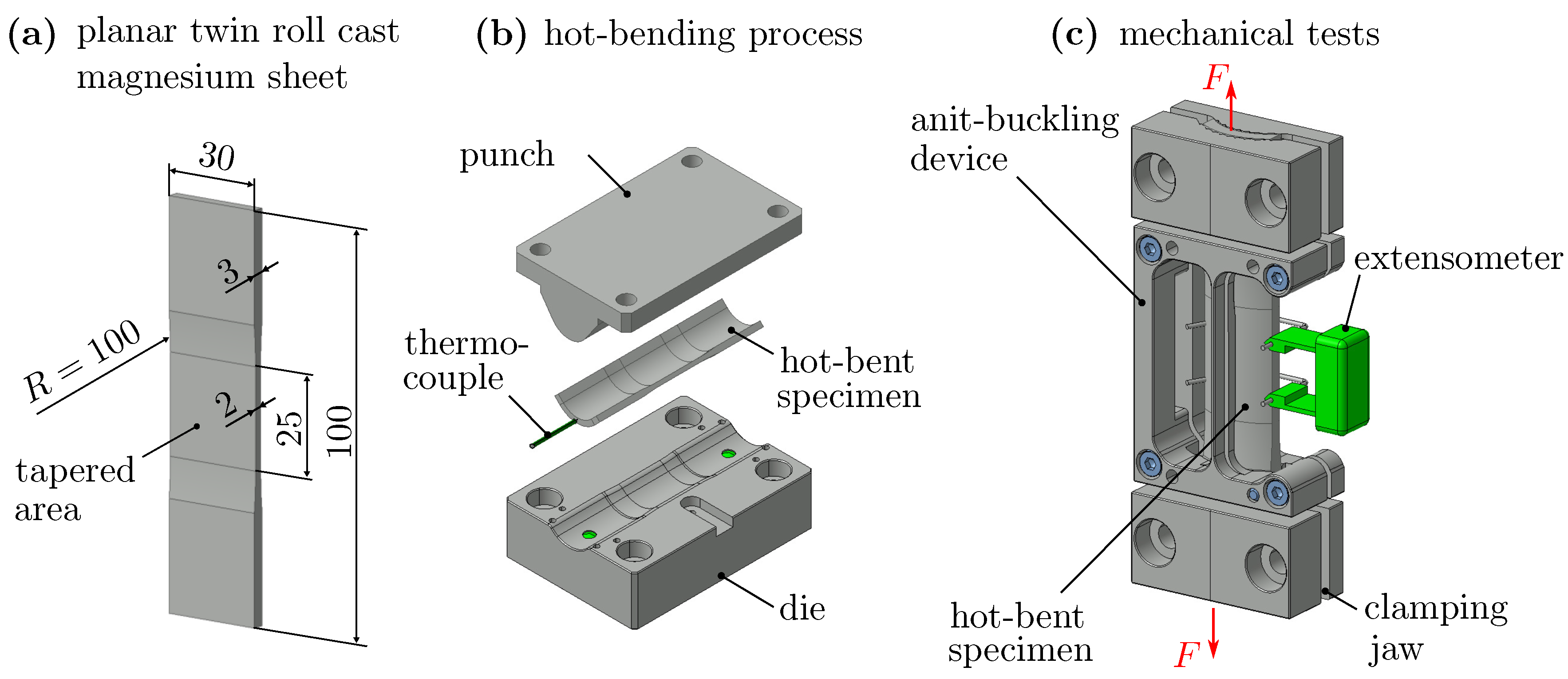
2.1. Hot-Bending Process

Hot-bent uniaxial specimens were made from a 3 $\mathrm{m}$$\mathrm{m}$-thick planar twin-roll cast AZ31B magnesium (Mg) sheet. The as-received sheets, with the chemical composition shown in

Table 1. Chemical composition of the AZ31B sheet metal in weight percent ($\mathrm{wt}\%$) [26].

Mg	Al	Zn	Mn	Cu	Si	Fe	Ni	Ca	Other Impurities
balance	2.75	1.08	0.368	0.00262	0.0187	0.00282	0.00038	0.00041	<0.004

, were manufactured by Magnesium Flachprodukte GmbH, Freiberg, Germany, with an average grain size of $5.1$ $\mathsf{\mu }$$\mathrm{m}$ and a strong basal texture [26].

Figure 1 shows the schematic manufacturing process of the hot-bent uniaxial specimens, starting with cutting the planar twin-roll Mg-sheet into 100 $\mathrm{m}$$\mathrm{m}$ × 25 $\mathrm{m}$$\mathrm{m}$ (length × width) pieces. The gauge section (tapered area) and the adjacent radii were manufactured by reducing the sheet thickness to 2 $\mathrm{m}$$\mathrm{m}$ using a milling process, as illustrated in Figure 1a.

Next, the planar Mg-sheets were hot-bent with a Langzauner LZT-OK-50-L heating press using the bending tool shown in Figure 1b. The punch and die were preheated by the heating press to the bending temperature $T_{\mathrm{B}}=235 {}^{\circ }\mathrm{C}$ without the planar Mg-sheet. Once the bending tool reached $T_{\mathrm{B}}$, the planar Mg-sheet was inserted, heated to $T_{\mathrm{B}}$, and bent. The feed rate and maximum bending force of the punch were set to $v_{\mathrm{f}}=0.5 \mathrm{m}\mathrm{m}/\mathrm{s}$ and $F_{\mathrm{B},\max }=20 \mathrm{k}\mathrm{N}$, respectively. As shown in Figure 1b, a thermocouple was attached to the end of the hot-bent uniaxial specimen, which ensures that $T_{\mathrm{B}}$ was reached. During the hot-bending process of all 13 specimens, the time $t_{\mathrm{T}>100 {}^{°}\mathrm{C}}$ in which the specimens have a temperature higher than 100 ${}^{°}\mathrm{C}$ was $182\pm 25$ $\mathrm{s}$. As shown in Figure 1c and Figure 2a, the specimens were machined laterally after the bending process to create two parallel surfaces for mounting the tactile extensometer.

The dimensions and manufacturing details of the hot-bent uniaxial specimen can be taken from Figure 2a. It should be mentioned that in this work, the axis system shown in Figure 2a is used, where the $x_1$-axis corresponds to the rolling direction (RD), the $x_2$-axis to the transverse direction (TD), and the $x_3$-axis to the normal direction (ND). The main objective of the curved, hot-bent specimen is a uniaxial homogeneous stress state in the gauge area without a superimposed bending stress. Therefore, the specimen was designed such that the $x_3$-coordinates of the centroid points $S_{x_3}^1=12.46 \mathrm{m}\mathrm{m}$ and $S_{x_3}^2=12.47 \mathrm{m}\mathrm{m}$ of the areas $A_1=55.26 \mathrm{m}{\mathrm{m}}^2$ and $A_2=36.81 \mathrm{m}{\mathrm{m}}^2$ are almost equal. Numerical simulations and experimental investigations of the loaded hot-bent specimen, concerning a uniaxial and homogeneous stress state, are discussed in Section 3.

2.2. Microstructural Investigations

Microstructural analyses were performed on both the as-received and the hot-bent materials with a Zeiss Merlin compact VP scanning electron microscope (SEM) equipped with an Oxford Instruments electron backscatter diffraction (EBSD) detector. EBSD patterns were measured with an acceleration voltage of 20 $\mathrm{k}$$\mathrm{V}$, a  120 $\mathsf{\mu }$$\mathrm{m}$ aperture, and at a working distance of ≈$9.5 \mathrm{m}\mathrm{m}$. The samples were fine ground with different SiC abrasive papers that had an average particle size from 25 $\mathsf{\mu }$$\mathrm{m}$ through to $2.5$ $\mathsf{\mu }$$\mathrm{m}$. A Buehler VibroMet 2 vibratory polishing machine with a chemical-resistant neoprene polishing cloth was used to polish the samples. In the first polishing stage, a  $0.02$ $\mathsf{\mu }$$\mathrm{m}$ SiO${}_2$-water suspension was used; for the final stage, a $0.04$ $\mathsf{\mu }$$\mathrm{m}$ Al${}_2$O${}_3$-ethanol suspension was taken. For analysis of the EBSD measurements, the software ATEX© [27] was used. All EBSD images were processed with a cleaning procedure, in which a full correction of up to 2 neighboring data points was performed. A minimum misorientation angle of 5° was used in the software to determine the grain boundaries.

2.3. Uniaxial Quasi-Static and Cyclic Tests at Room Temperature

For the strain-controlled uniaxial tests at room temperature, a uniaxial servo-hydraulic test rig with a 25 $\mathrm{k}$$\mathrm{N}$ Schenk cylinder, a  25 $\mathrm{k}$$\mathrm{N}$ Interface load cell, and a Sandner EXA10-10 extensometer was used. The test rig for the quasi-static and cyclic tests is shown in Figure 2b. Figure 1c and Figure 2b show the mechanical test setup, consisting of the hot-bent uniaxial specimen, the extensometer and the anti-buckling device, which prevents the specimen from buckling under compressive load. A self-adhesive PTFE-foil was attached to the inner surfaces of the anti-buckling device to reduce friction. Specimen-shaped compatible clamping jaws enable the integration of the hot-bent uniaxial specimen into the servo-hydraulic test rig.

The low-cycle fatigue tests were conducted with constant strain amplitude loading and an extensometer strain ratio $R_{\epsilon ,\mathrm{ext}}=-1$. In situ strain field measurements with digital image correlation (DIC) were made with the GOM Aramis 12 M optical strain field measurement system during fatigue testing. Images were taken from the upper, lower, and mean load level at approximately half of the fatigue life $N_f/2$ and analyzed with custom-developed software in Python™ 3.8.5. For the determination of $N_f$, the initial stiffness of the hot-bent uniaxial specimen was calculated by the digital control system EU3000RTC from Inova and continuously compared with the actual stiffness of the cycle. The number of cycles to failure $N_f$ was defined as the number of cycles for which the actual stiffness was 5% below the initial stiffness.

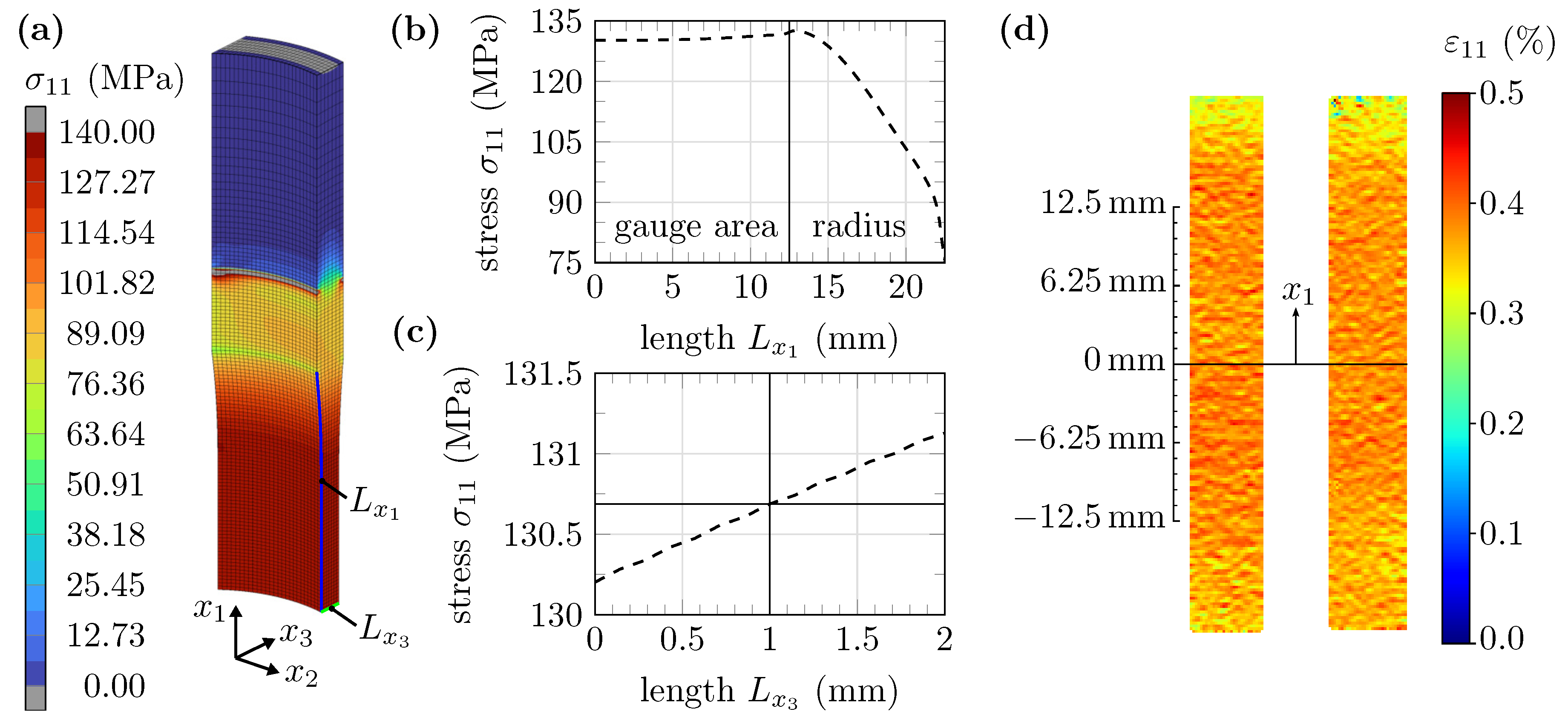
3. Numerical and Experimental Verification of the Novel, Hot-Bent Uniaxial Specimen

The curved, hot-bent specimen was designed using the finite element method (FEM) calculations to achieve a specimen with a uniaxial and homogeneous stress state. This was verified, as illustrated in Figure 3a–c, by means of the analysis of the stress field ${\sigma }_{11}(x_1,x_2,x_3)$ via FEM calculations. Two symmetry planes, the $x_1$-$x_3$- and $x_2$-$x_3$-planes, were used to build the geometry model, leaving only the upper-left quarter of the specimen from Figure 2a. It should be mentioned that the same coordinate system is used in the FEM simulation and in Figure 2a. A total number of 21,658 hexahedral elements with quadratic shape functions are used for the discretization and approximation of the geometry and the displacement field. The symmetry boundary conditions $u_1=0$ and $u_2=0$ were defined for the $x_2$-$x_3$- and $x_1$-$x_3$-symmetry-plane, respectively. A reference node was defined at $x_1=36 \mathrm{m}\mathrm{m}$, $x_2=0 \mathrm{m}\mathrm{m}$, and $x_3=12.47 \mathrm{m}\mathrm{m}$. This corresponds to the centroid point $S_{x_i}^1$ of the cross-sectional area $A_1$ of the clamping area shown in Figure 2a. The nodes of the two clamping surfaces were kinematically coupled with the reference node, for which the displacement boundary conditions $u_i=0$$(i=2,\cdots ,6)$ were defined. In the $u_1$-direction, the reference node was defined as freely displaceable. Finally, a tensile force of $F_1=2392 \mathrm{N}$ was applied to the reference node, resulting in a tensile stress of ${\sigma }_{11}=MM{F}_1/2A_2\approx 130 \mathrm{M}\mathrm{Pa}$ in the gauge cross-section $A_2$. A linear, elastic model was used with a Young’s modulus of E = 41,067 MPa and Poisson’s ratio $\nu =0.3$. The values E and $\nu$ of the hot-bent material were determined in a quasi-static test, which is discussed in more detail in Section 4.2. Geometric nonlinearity was taken into account in the FEM simulation.

Figure 3a represents the normal stress field ${\sigma }_{11}(x_1,x_2,x_3)$ of the FEM analysis. From the plotted stress field ${\sigma }_{11}(x_1,x_2,x_3)$ of Figure 3a, a homogeneous stress ${\sigma }_{11}$ is observed with no evident stress concentrations in the gauge area. In Figure 3b, the stress ${\sigma }_{11}$ is plotted along the path $L_{x_1}$, which is indicated in Figure 3a. It can be proven that the highest stress ${\sigma }_{11}(x_1=0 \mathrm{m}\mathrm{m}, x_2=0 \mathrm{m}\mathrm{m}, x_3=12.5 \mathrm{m}\mathrm{m})\approx 130.2 \mathrm{M}\mathrm{Pa}$ is within the gauge area. Only in the transition zone between the gauge area and the radius, a negligible stress increase of 1.87% is obtained. It should be noted that stress concentrations caused by the modeled boundary conditions at the clamping area are not taken into account, since—according to the principle of St. Venant—disturbances decay rapidly. A further plot, shown in Figure 3c, where the stress ${\sigma }_{11}$ is plotted along the path $L_{x_3}$, illustrates that only a small bending stress of ≈$0.5 \mathrm{M}\mathrm{Pa}$ is superimposed.

A strain field measurement was performed using the digital image correlation method to experimentally verify the homogeneity of the strain field ${\epsilon }_{11}(x_1,x_2)$. Figure 3d shows the measured strain field of the uniaxial specimen at an extensometer strain ${\epsilon }_{11,\mathrm{ext}}=0.45\%$, with the middle part hidden by the anti-buckling device. The analysis confirms that the strain field is homogeneous in the gauge area.

A further experimental investigation with a strain-controlled tension test was conducted to determine the superimposed bending stress. For this purpose, strain gauges were glued to the inner radius $R_{\mathrm{inner}}=12.5 \mathrm{m}\mathrm{m}$ and outer radius $R_{\mathrm{outer}}=14.5 \mathrm{m}\mathrm{m}$ of the gauge area. The corresponding strain at the inner ${\epsilon }_{11,\mathrm{inner}}$ and outer ${\epsilon }_{11,\mathrm{outer}}$ radius was measured via the strain gauges. With ${\epsilon }_{11,\mathrm{inner}}$ and ${\epsilon }_{11,\mathrm{outer}}$, the bending stress ${\sigma }_{11,\mathrm{B}}=MME/2\left({\epsilon }_{11,\mathrm{outer}}-{\epsilon }_{11,\mathrm{inner}}\right)$ is calculated, which is listed in

Table 2. Results of the strain-controlled tension test, in which the strain at the outer radius ${\epsilon }_{11,\mathrm{outer}}$ and inner radius ${\epsilon }_{11,\mathrm{inner}}$ in the gauge area are measured with strain gauges to determine the superimposed bending stress ${\sigma }_{11,\mathrm{B}}$.

${\mathit{\epsilon }}_{11,\mathbf{ext}}$ (%)	${\mathit{\sigma }}_{11}$ (MPa)	${\mathit{\epsilon }}_{11,\mathbf{outer}}$ (%)	${\mathit{\epsilon }}_{11,\mathbf{inner}}$ (%)	${\mathit{\sigma }}_{11,\mathbf{B}}$ (MPa)
0.100	41.1	0.100	0.0900	2.05
0.200	82.1	0.210	0.180	6.16
0.300	123	0.320	0.290	6.16

. For ${\epsilon }_{11,\mathrm{ext}}=0.3\%$, a bending stress of ${\sigma }_{11,\mathrm{B}}=6.16 \mathrm{M}\mathrm{Pa}$ is calculated, which corresponds to 5% of the normal stress. The discrepancy between the numerical simulation and the experimental result can be explained by manufacturing tolerances of the specimen. However, the 5% superimposed bending stress is tolerable and can be neglected to a good approximation.

In summary, the FEM results, the strain field measurement, and the tension test with attached strain gauges demonstrate that a homogeneous and uniaxial stress state can be realized in the gauge area of the hot-bent specimen. The superimposed bending stress is tolerable. The specimen can thus be used to investigate to which extent the hot-bending process changes the quasi-static and cyclic mechanical properties.

4. Results and Discussion

Since there are microstructural changes due to the hot-bending process [21,25], microstructural analyses of the hot-bent material are shown in this section and compared with results for the as-received material. Subsequently, the microstructural findings help to understand the different mechanical properties for as-received and hot-bent material.

4.1. Microstructural Analyses

Figure 4a–c show EBSD orientation maps with a view in the ND of the as-received material and the hot-bent material to investigate the evolution of the microstructure on both the tension and compression layer of the bending radius. These measurements were made from smaller areas with high resolution and small scan steps to accurately examine the microstructure, such as grain boundaries. The as-received material, analyzed in Figure 4a, has a homogeneous microstructure with smooth grain boundaries and an average grain size of ≈$5.1 \mathsf{\mu }\mathrm{m}$.

Due to low-temperature dynamic recrystallization [28], the hot-bent material developed an inhomogeneous microstructure with deformed and serrated grain boundaries. This can be observed from the EBSD maps of the tension (Figure 4b) and compression (Figure 4c) layers. Numerous small grains are formed, which are detected in Figure 4b,c in the regions ($x_1=35 \mathsf{\mu }\mathrm{m},x_2=40 \mathsf{\mu }\mathrm{m}$) and ($x_1=15 \mathsf{\mu }\mathrm{m},x_2=10 \mathsf{\mu }\mathrm{m}$), respectively. On the other hand, a few large grains are formed, as it can be seen in Figure 4c at ($x_1=30 \mathsf{\mu }\mathrm{m},x_2=45 \mathsf{\mu }\mathrm{m}$). The average grain size is about $3.8 \mathsf{\mu }\mathrm{m}$ for the tension layer and about $3.5 \mathsf{\mu }\mathrm{m}$ for the compression layer.

In order to improve the statistical accuracy, further EBSD measurements were carried out with a scan size of $540 \mathsf{\mu }\mathrm{m}$ × $225 \mathsf{\mu }\mathrm{m}$ (TD × RD), corresponding to a statistically representative area (>4600 grains). Figure 5a–c show the determined (0002) pole figures of the EBSD measurements from the as-received material and the hot-bent material of the tension and the compression layer, respectively. According to the pole Figure 5a, the typical {0002} ⊥ ND basal texture can be confirmed for the as-received material with a maximum intensity of approximately 14.92. In contrast, the texture from the hot-bent material of the tension layer, shown in Figure 5b, is weakened by a factor of approximately 2.05. The texture randomization is more pronounced in the compression layer compared with the tension layer, which leads to a slightly inhomogeneous texture throughout the sheet thickness. Related to the as-received material, the basal texture of the compression layer is weakened by a factor of approximately 2.89. Figure 5b,c clearly show that the hot-bending process changes the texture by tilting the c-axes from ND towards TD. This grain inclination is slightly higher for the compression layer.

According to [28], basal <a>, prismatic <a>, pyramidal <a>, or pyramidal <a + c> slip are activated in the tension layer during the hot-bending process. In the compression layer, $\left\{10\overline{1}2\right\}$ tension twins are additionally activated for the plastic deformation [28]. Therefore, a further EBSD measurement of the compression layer, shown in Figure 6a, was performed to investigate if $\left\{10\overline{1}2\right\}$ tension twins form. The misorientation angle of (86.3 ± 5)° between a $\left\{10\overline{1}2\right\}$ tension twin and its parent grain is used in Figure 6b as a detection criterion for twins. Based on the analysis, $\left\{10\overline{1}2\right\}$ tension twins are identified, which are marked in blue within Figure 6b, e.g., at $(x_1=2.5 \mathsf{\mu }\mathrm{m},x_2=17.5 \mathsf{\mu }\mathrm{m})$. The twin formation could be the main cause for the rotation of the c-axes towards TD. This also explains why the c-axes rotation is slightly less pronounced on the tension layer (Figure 5b), since mainly dislocation slip occurs for a tensile stress. Furthermore, the tilt is mainly in TD and not in RD, which results from the load-direction-guided twin formation. A similar behavior for the texture evolution of hot-bent AZ31B could already be observed in [23].

This texture evolution affects the Schmid factor for basal slip $M_{\left(0002\right)}$ with respect to a possible load in TD or RD. Figure 7a,b show the Schmid factor maps for basal slip of the as-received material loaded in RD and TD, respectively. In both directions, the average Schmid factor is ${\overline{M}}_{\left(0002\right)}\approx 0.16$, which is relatively low. As a consequence, yielding at room temperature of the as-received material in tension and compression along RD or TD is dominated by prismatic slip and $\left\{10\overline{1}2\right\}$ tension twins, respectively [7].

Figure 7c–f show the Schmid factor maps for basal slip for a possible load in RD and TD of the hot-bent material from the tension and compression layer, respectively. The average Schmid factor in RD for the compression layer is ${\overline{M}}_{\left(0002\right),\mathrm{RD}}\approx 0.2$, which corresponds to an increase of 25% compared with the as-received material. The average Schmid factor in TD is ${\overline{M}}_{\left(0002\right),\mathrm{TD}}\approx 0.33$, which corresponds to a significant increase of 87.5% compared with the as-received material. This significant increase in the Schmid factor in TD is seen in Figure 7f.

In summary, the hot-bending process leads to significant changes in the microstructure with a smaller average grain size and deformed grain boundaries. The c-axes become inclined from ND towards TD, which is more pronounced on the compression layer compared with the tension layer due to two effects. First, the slight inclination of the c-axes towards TD is explained by dislocation slip and grain rotation. Second, the rotation of approximately 86.3° in TD results from $\left\{10\overline{1}2\right\}$ tension twins, which are slightly more prevalent in the compression layer. Hence, the Schmid factor for basal slip in RD and TD increases, which may have an influence on the mechanical quasi-static and cyclic material properties. In the following, the novel, uniaxial specimen, introduced in Section 2, will be used to investigate the influence of the microstructural changes on the quasi-static and cyclic material properties.

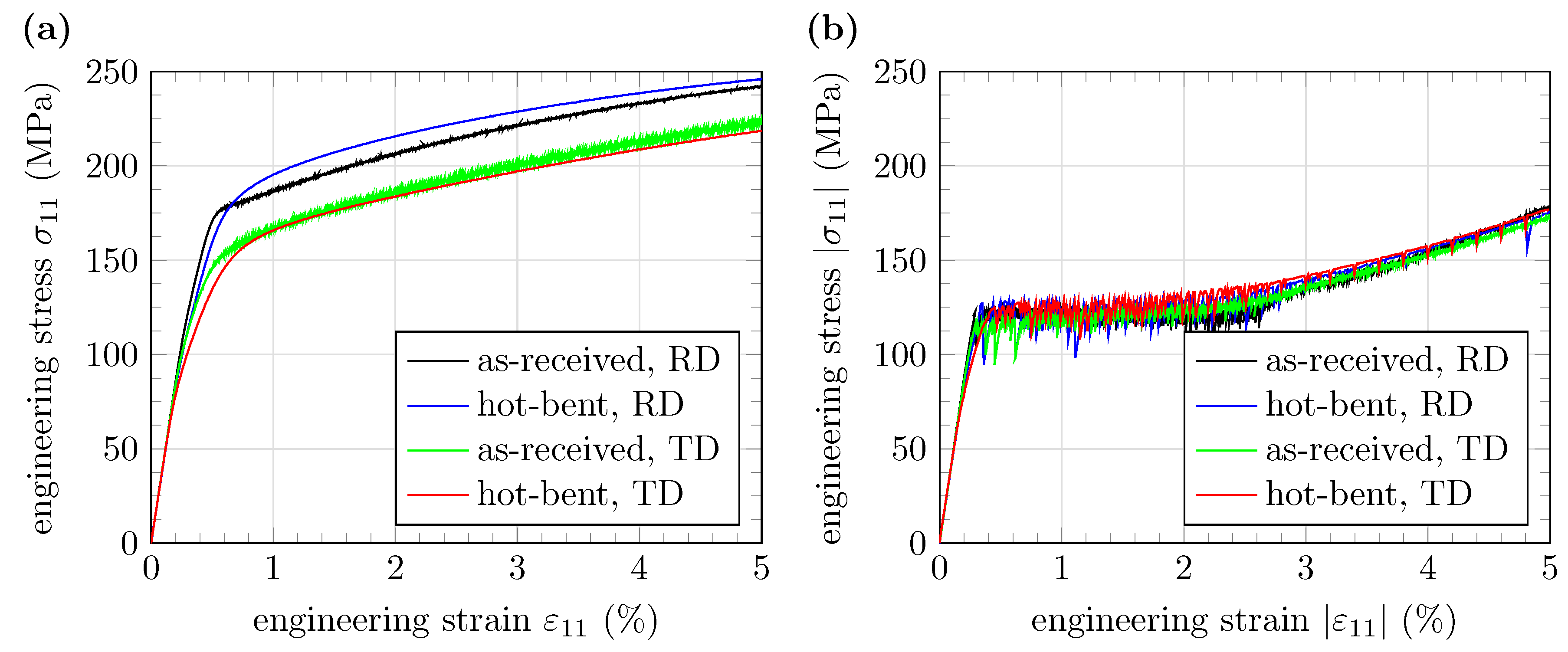
4.2. Quasi-Static Tests

In order to analyze the effects of the microstructural changes due to the hot-bending process, strain controlled uniaxial tension and compression tests were performed in RD and TD and the result compared with the as-received material. In Figure 8a,b, the engineering stress–strain curves of the tension and compression tests are plotted. The typical asymmetry between the tensile and compressive yield stresses ${\sigma }_{\mathrm{Y}}$ is observed [8], which is valid for both the as-received material and the hot-bent material. In addition, anisotropic tensile yield stresses are obtained for RD and TD, with the tensile yield stress in TD being on average about 17.5% lower than the yield stress in RD. In contrast, no such distinctive anisotropy is found for the compressive yield stresses.

AZ31B has an almost ideal plastic material behavior up to ${\epsilon }_{11,\mathrm{ext}}\gtrsim -2.5\%$ in the compression test because of the formation of $\left\{10\overline{1}2\right\}$ tension twins. Additionally, the typical serrated flow is observed due to twinning in the compression tests [12]. However, for the hot-bent material, there is a slight increase for the work hardening due to the microstructure evolution, which was discussed in Section 4.1.

For the numerical comparison between the as-received and hot-bent material, the yield stresses ${\sigma }_{\mathrm{Y}}$ and the Young’s moduli E are listed in

Table 3. Results of the yield stresses ${\sigma }_{\mathrm{Y}}$ and the Young’s moduli E from the uniaxial tension and compression tests. These tests are carried out with the as-received and the hot-bent material in RD and TD.

	Uniaxial Tension Tests		Uniaxial Compression Tests
ID	${\mathbf{\sigma }}_{\mathbf{Y}}$ (MPa)	$\mathit{E}$ (MPa)	$|{\mathbf{\sigma }}_{\mathbf{Y}}|$ (MPa)	$\mathit{E}$ (MPa)
hot-bent, RD	177.1	41,067	128.3	40,862
as-received, RD	178.1	42,673	122.8	43,880
hot-bent, TD	142.5	38,945	124.9	38,422
as-received, TD	150.6	42,034	116.4	42,879

. Young’s moduli E were computed by performing a linear regression with the measured stress and strain values between $0.05\%\le {\epsilon }_{11,\mathrm{ext}}\le 0.2\%$, where the slope of the linear function corresponds to E. It is found that the tensile yield stresses of the as-received material are slightly higher than that of the hot-bent material. Contrarily, the compressive yield stresses of the as-received material are smaller than those of the hot-bent material. Another observation concerns the Young’s modulus E. By comparison with the as-received material, E is lower for all hot-bent specimens, especially along TD. For example, the Young’s modulus of the hot-bent specimen is ≈$10.4\%$ lower in TD compared with that of the as-received material. This effect can be observed in Figure 8a, since the stress–strain curves of the hot-bent specimens already show a slight nonlinearity between $50 \mathrm{M}\mathrm{Pa}\lesssim {\sigma }_{11}\lesssim {\sigma }_{\mathrm{Y}}$. Such behavior can be attributed to microstructural changes during hot-bending, since dislocations and tension twins are induced by the plastic deformation of the process. These additional dislocations and tension twins are released or detwinned in the tension tests at lower stresses, resulting in nonlinearity and lower Young’s modulus.

Recent investigations [12,17,18,26] have shown that due to the dominant formation of tension twins, macroscopic bands of twinned grains (BTGs) are forming under compressive load in the sheet plane. Within the BTGs, the compressive strain is much higher compared with the regions outside the bands. Figure 9 shows the strain field ${\epsilon }_{11}(x_1,x_2)$ of a hot-bent specimen from a compression test at an extensometer strain ${\epsilon }_{11,\mathrm{ext}}=-0.45\%$. The center region of the specimen is covered by the anti-buckling device.

The experiment demonstrates that with the hot-bent material, similar to the as-received material, macroscopic BTGs are formed in the gauge area. For the as-received material, the BTG boundaries are almost perfectly perpendicular to the load direction [17]. However, this is not as distinctive for the hot-bent material. A possible explanation could be the texture evolution discussed in Section 4.1. In the hot-bent material, unlike the as-received material, the c-axes of the grains are inclined from ND towards TD and slightly towards RD. In these grains, twinning is less likely. The horizontal propagation front ($x_2$-direction) of the BTG boundaries moves along the grains in which the c-axes are oriented favorably for twinning.

Three results can be obtained from the uniaxial tension and compression tests. First, the asymmetric and anisotropic elasto-plastic material behavior do not change significantly due to the hot-bending process. Second, the hot-bent specimens exhibit lower Young’s moduli than the specimens from the as-received material. Third, even in the hot-bent specimens, the massive formation of tension twins during the compression tests causes macroscopic bands of twinned grains. Within the BTGs, the compressive strain $|{\epsilon }_{11}|$ is considerably higher compared with the areas outside the BTGs.

4.3. Low-Cycle Fatigue Tests

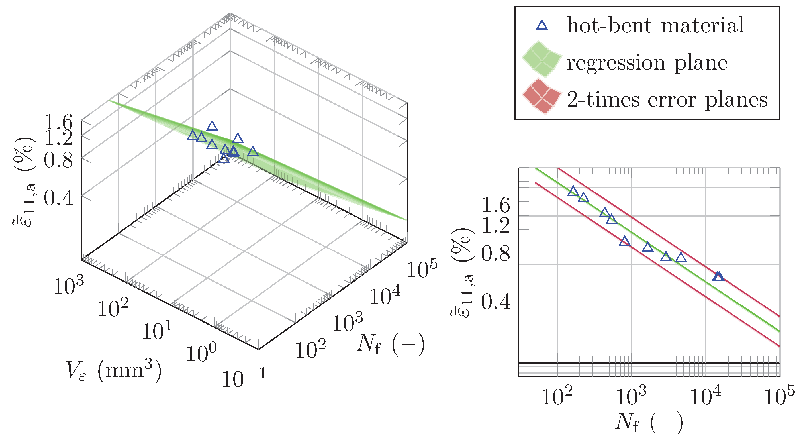
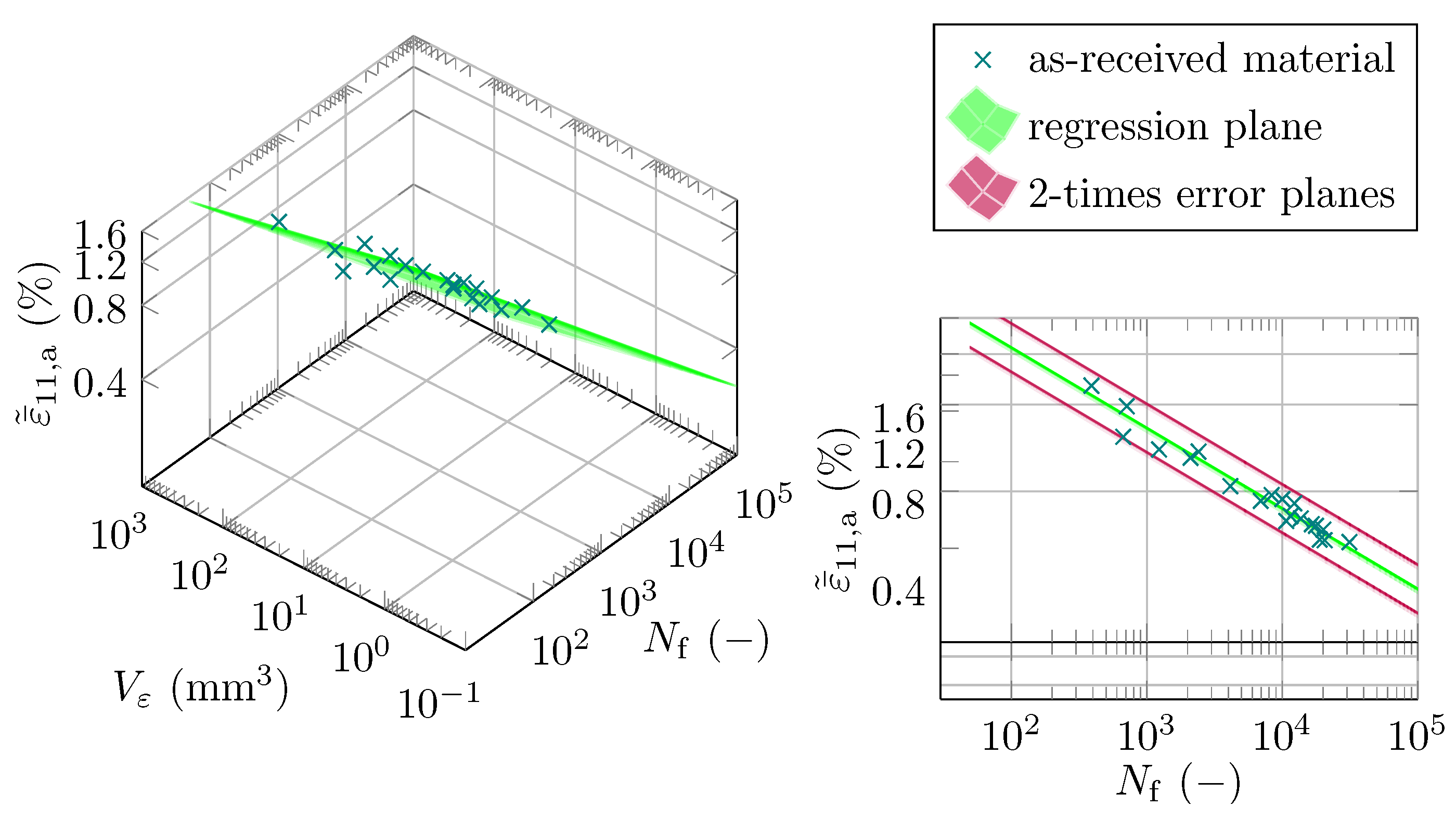
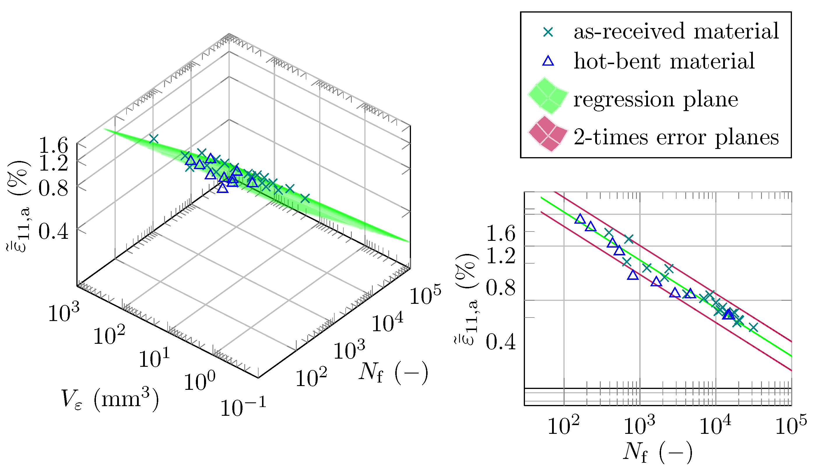
4.3.1. The Concept of Highly Strained Volume

Owing to the basal texture, the massive twin formation, and the almost ideal plastic material behavior during twinning, macroscopic BTGs are formed in which the compressive strain $|{\epsilon }_{11}|$ is considerably higher compared with regions outside the BTGs. It is shown in [16,26] that the common fatigue parameters, e.g., the strain amplitude ${\epsilon }_{\mathrm{a}}$, are higher in the BTGs. Therefore, in all fatigue tests, the first macroscopic crack is localized in a BTG. In order to consider all these aspects in a fatigue model, the concept of highly strained volume (CH$\epsilon$V) was proposed in [26]. In the following, the CH$\epsilon$V is applied to the hot-bent specimens and compared with the results of the as-received material from [16,26]. Finally, this investigation verifies whether the CH$\epsilon$V is applicable to Mg-structures that are hot-bent.

The determination of the highly strained Volume $V_{\epsilon }$ is divided into three main steps. First, the highly strained region (HSR) is separated from the strain field ${\epsilon }_{11}(x_1,x_2){|}_{\mathrm{LLL}}$ at the lower load level (LLL) measured by DIC. Therefore, the minimum value ${\epsilon }_{11,\min }{|}_{\mathrm{LLL}}$ of the entire strain field at LLL ${\epsilon }_{11}(x_1,x_2){|}_{\mathrm{LLL}}$ is calculated in order to determine the threshold strain

$${\epsilon }_{11,\mathrm{thr}}{{|}_{\mathrm{LLL}}=0.8{\epsilon }_{11,\min }|}_{\mathrm{LLL}}.$$

(1)

The HSR consists of the measurement facets k of the strain field ${\epsilon }_{11}(x_1,x_2){|}_{\mathrm{LLL}}$, which fulfill the condition ${\epsilon }_{11}(x_1,x_2){{|}_{\mathrm{LLL}}\le {\epsilon }_{11,\mathrm{thr}}|}_{\mathrm{LLL}}$.

Second, the highly strained region with high strain amplitude (HSRA) is separated from the HSR. Effective quantities from the HSR are indicated with $\left(\tilde{\blacksquare }\right)$. Therefore, the effective strain amplitudes

$${\tilde{\epsilon }}_{11,\mathrm{a}}(x_1,x_2)=\frac{1}{2}\left({\tilde{\epsilon }}_{11}(x_1,x_2){{|}_{\mathrm{ULL}}-{\tilde{\epsilon }}_{11}(x_1,x_2)|}_{\mathrm{LLL}}\right)$$

(2)

are calculated with the effective strain field at the upper load level (ULL) ${\tilde{\epsilon }}_{11}(x_1,x_2){|}_{\mathrm{ULL}}$ and the LLL ${\tilde{\epsilon }}_{11}(x_1,x_2){|}_{\mathrm{LLL}}$. When calculating the maximum effective strain amplitude

$${\tilde{\epsilon }}_{11,\mathrm{a},\max }=\max \left[{\tilde{\epsilon }}_{11,\mathrm{a}}(x_1,x_2)\right]$$

(3)

from the entire effective strain amplitude field, the HSRA is separated by defining a threshold strain amplitude

$${\tilde{\epsilon }}_{11,\mathrm{a},\mathrm{thr}}=0.7{\tilde{\epsilon }}_{11,\mathrm{a},\max }.$$

(4)

For the separation of the HSR and HSRA from the DIC measurements, Equations (1)–(4) were implemented in a custom-developed software programmed with Python™.

In the third and last step, the fatigue parameter $V_{\epsilon }$ is calculated with the Python™ software from the area of the remaining HSRA and the specimen thickness. Additionally, the mean effective strain amplitude ${\tilde{\overline{\epsilon }}}_{11,\mathrm{a}}$ of the HSRA is determined. It should be noted that $V_{\epsilon }$ and ${\tilde{\overline{\epsilon }}}_{11,\mathrm{a}}$ are evaluated at half of fatigue life $MM{N}_{\mathrm{f}}/2$, where stabilized material behavior can be assumed [17]. For a more detailed description of the CH$\epsilon$V, the reader is referred to [16,26].

4.3.2. Fatigue Modeling

In this paragraph, the CH$\epsilon$V is applied to the hot-bent specimens and compared with data from uniaxial specimens fabricated from the as-received material. Therefore, strain-controlled cyclic tests with an extensometer strain ratio $R_{\epsilon ,\mathrm{ext}}=-1$ were performed on ten hot-bent specimens.

Table 4. Applied extensometer strain amplitude ${\epsilon }_{\mathrm{a},\mathrm{ext}}$, extensometer strain ratio $R_{\epsilon }$, test frequency f, highly strained volume $V_{\epsilon }$, mean effective strain amplitude ${\tilde{\overline{\epsilon }}}_{11,\mathrm{a}}$, and the numbers of cycles to failure $N_{\mathrm{f}}$ of the strain-controlled cyclic tests. The tests are performed on the hot-bent specimens.

Specimen ID	${\mathit{\epsilon }}_{\mathbf{a},\mathbf{ext}}$ (%)	${\mathit{R}}_{\mathit{\epsilon }}$(−)	f (Hz)	${\mathit{V}}_{\mathit{\epsilon }}$ (mm3)	${\widetilde{\overline{\mathit{\epsilon }}}}_{11,\mathbf{a}}$ (%)	${\mathit{N}}_{\mathbf{f}}$ (−)
UG12-060	0.35	−1	1	132	0.344	14,377
UG12-061	0.35	−1	1	523	0.334	15,075
UG12-062	0.45	−1	0.5	43.0	0.469	2890
UG12-063	0.45	−1	0.5	23.3	0.470	4619
UG12-065	0.55	−1	0.2	24.4	0.595	807
UG12-071	0.55	−1	0.2	81.7	0.532	1645
UG12-067	0.8	−1	0.1	46.5	0.885	435
UG12-072	0.8	−1	0.1	16.0	0.822	535
UG12-068	1.2	−1	0.1	32.2	1.21	163
UG12-070	1.2	−1	0.1	4.99	1.15	224

lists the applied extensometer strain amplitudes ${\epsilon }_{\mathrm{a},\mathrm{ext}}$, the test frequencies f, the highly strained volumes $V_{\epsilon }$, the mean effective strain amplitudes ${\tilde{\overline{\epsilon }}}_{11,\mathrm{a}}$ and the numbers of cycles to failure $N_{\mathrm{f}}$ of the cyclic tests. Two repetitions for the respective extensometer strain amplitude ${\epsilon }_{\mathrm{a},\mathrm{ext}}$ were performed. The data from the cyclic tests of the as-received material are taken from [26].

The parameters $V_{\epsilon }$, ${\tilde{\overline{\epsilon }}}_{11,\mathrm{a}}$, and $N_{\mathrm{f}}$ are plotted in a three-dimensional graph with logarithmic scales. Figure 10 shows the 3D ${\tilde{\overline{\epsilon }}}_{11,\mathrm{a}}$-$V_{\epsilon }$-$N_{\mathrm{f}}$ fatigue diagram with the data points marked with triangles and a 2D projection view of ${\tilde{\overline{\epsilon }}}_{11,\mathrm{a}}$ vs. $N_{\mathrm{f}}$. The 2D projection is in the $V_{\epsilon }$ viewing direction and slightly tilted around the $N_{\mathrm{f}}$ axis so that the 2-times error planes are parallel to the viewing direction. The nonlinear Levenberg–Marquardt least square algorithm scipy.optimize.curve_fit from SciPy© is used to fit the experimental data to the double power function

$${\tilde{\overline{\epsilon }}}_{11,\mathrm{a}}(N_{\mathrm{f}},V_{\epsilon })=C_1{N}_{\mathrm{f}}^{d_1}{\left(\frac{V_{\epsilon }}{{\mathrm{m}}^3\mathrm{m}}\right)}^{d_2}.$$

(5)

The algorithm minimizes the sum of squares of the nonlinear Equation (5) by optimizing the coefficient $C_1$ and the exponents $d_1$ and $d_2$ until the function fits the measured data. Both the coefficient $C_1$ and the exponents $d_1$ and $d_2$ are material parameters. Ultimately, this leads to the regression plane plotted with green color in Figure 10. In addition, the 2-times error planes with respect to the $N_{\mathrm{f}}$-axis are plotted in the 2D projection view of Figure 10. All experimental data points lie within the two 2-times error planes, proving that the CH$\epsilon$V is well-suited to model the fatigue behavior of hot-bent AZ31B. The high value for the coefficient of determination $r^2=0.968$ of the regression analysis, listed in

Table 5. Determined material values $C_1$, $d_1$, and $d_2$ for the hot-bent material, the as-received material, and the combination of the hot-bent and as-received material. In addition, the coefficient of determination $r^2$ is given to estimate the quality of the regression.

Specimens	${\mathit{C}}_1$ (%)	${\mathit{d}}_1$ (−)	${\mathit{d}}_2$ (−)	${\mathit{r}}^2$ (−)
hot-bent	6.13	−0.310	−0.0189	0.968
as-received	6.30	−0.279	−0.0460	0.942
hot-bent & as-received	4.94	−0.266	−0.0231	0.944

, demonstrates the good approximation of the data points with the CH$\epsilon$V.

The plot of the experimental data and the regression plane for uniaxial specimens from the as-received material are presented in Figure 11. Once again, all experimental data points are within the two 2-times error planes, resulting in a relatively high coefficient of determination $r^2=0.942$. The $r^2$ value is slightly smaller compared with the value of the hot-bent specimens due to the larger number and variance of specimens from the as-received material.

Table 5 lists the determined material values $C_1$, $d_1$, and $d_2$ of the hot-bent and as-received material for the fatigue model from Equation (5). The deviation between the respective material properties can be attributed to the changing microstructure of the hot-bent material. It can be observed that the hot-bent material tends to have a lower number of cycles to failure $N_{\mathrm{f}}$.

Geometrically complex Mg-components, such as those used in the automotive industry, contain hot-bent and non-hot-bent regions [1]. Taking this into account, the experimental data of the hot-bent and the as-received material are combined and the CH$\epsilon$V is applied to the data. The result of the fatigue modeling is shown in the 3D and 2D ${\tilde{\overline{\epsilon }}}_{11,\mathrm{a}}$-$V_{\epsilon }$-$N_{\mathrm{f}}$ fatigue diagrams from Figure 12, where almost all data points lie within the two 2-times error planes. The material values $C_1$, $d_1$, and $d_2$ of the combined data, listed in Table 5, are different from the values of the hot-bent and the as-received material, respectively. This numerical difference results from the combination of the two materials. The high coefficient of determination value $r^2=0.944$ shows that the CH$\epsilon$V can accurately estimate the lifetime, even combining the as-received and hot-bent specimens in one model.

5. Conclusions

The complex quasi-static and cyclic material behavior of planar twin-roll cast AZ31B alloy sheets has been successfully investigated and modeled in previous studies. However, geometrically complex components are usually hot-bent, whereby the microstructure in the hot-bent areas changes significantly but studies on the mechanical material properties of hot-bent AZ31B magnesium alloy are currently lacking. Consequently, a novel, hot-bent uniaxial specimen is proposed. Microstructural investigations of the hot-bent specimens show the influence of the microstructural changes on the quasi-static and cyclic material behavior.

• Numerical and experimental results of the hot-bent specimen show that a homogeneous and uniaxial stress state with a tolerable low superimposed bending stress of 5% in the gauge area can be realized.
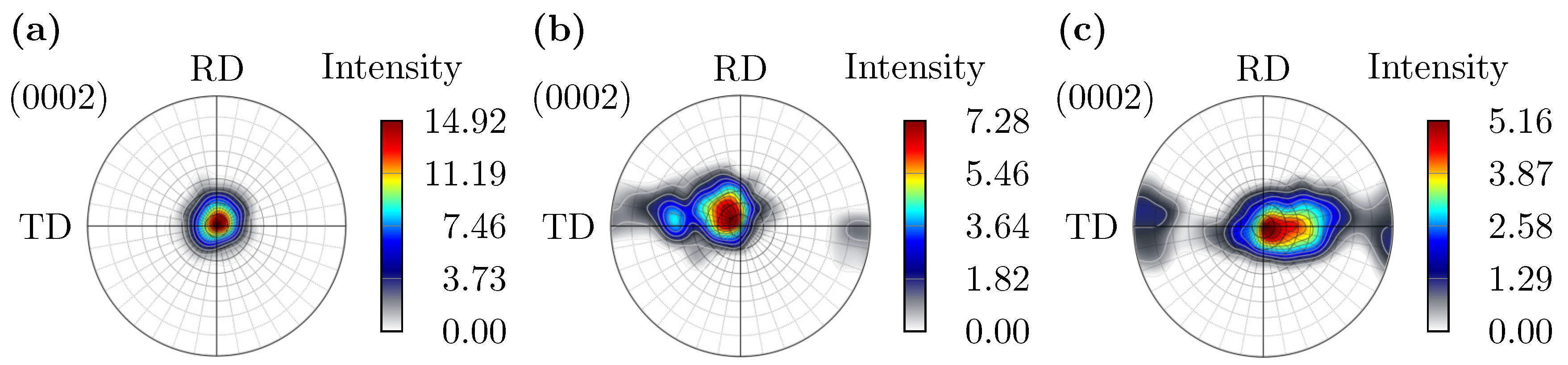
• The hot-bending process leads to changes in the microstructure with a smaller average grain size and deformed grain boundaries. Furthermore, it is observed that the c-axes become inclined from the normal direction (ND) towards the transverse direction (TD), which is more pronounced on the compression layer compared with the tension layer due to the formation of $\left\{10\overline{1}2\right\}$ tension twins. Hence, the Schmid factor for basal slip in RD and TD increases.
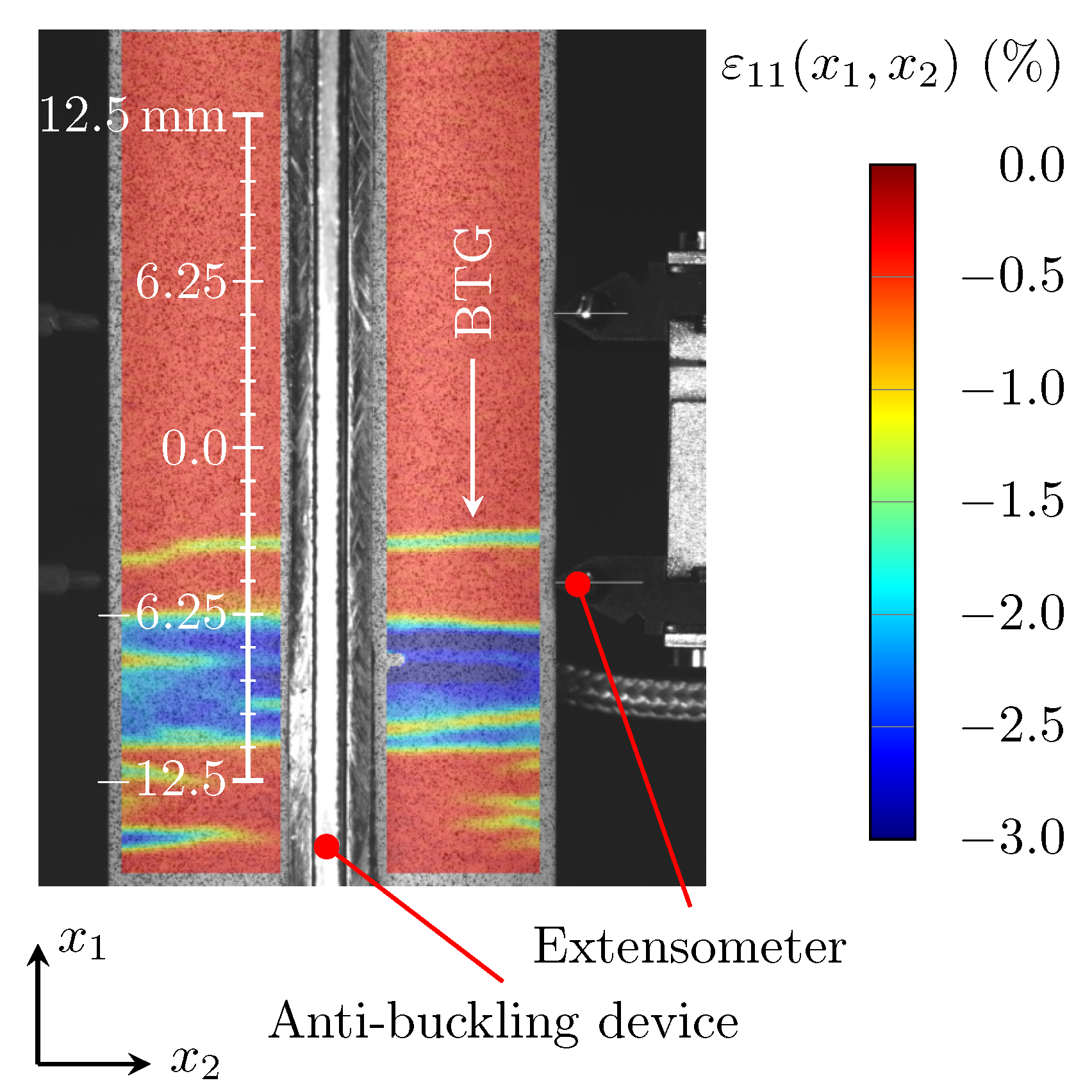
• The uniaxial tension and compression tests reveal that the anisotropic and asymmetric elasto-plastic material behavior persists after the hot-bending process. In addition, lower Young’s moduli are observed for the hot-bent material compared with the as-received material. Compression tests show that even in the hot-bent specimens, the massive formation of tension twins causes macroscopic bands of twinned grains (BTGs). Within the BTGs, the compressive strain $|{\epsilon }_{11,\mathrm{BTG}}|$ is considerably higher compared with the areas outside the BTGs.
• Finally, the study proves that the recently proposed concept of highly strained volume (CH$\epsilon$V) can accurately estimate the lifetime of as-received and hot-bent AZ31B magnesium alloy, even by combining the two materials in one model. This allows the CH$\epsilon$V to be applied to geometrically complex hot-bent components in order to estimate their lifetime.

References

1. Kulekci, M.K. Magnesium and its alloys applications in automotive industry. Int. J. Adv. Manuf. Technol. 2008, 39, 851–865. [Google Scholar] [CrossRef]
2. Mordike, B.L.; Ebert, T. Magnesium Properties—Applications—Potential. Mater. Sci. Eng. A 2001, 302, 37–45. [Google Scholar] [CrossRef]
3. Ucuncuoglu, S.; Ekerim, A.; Secgin, G.O.; Duygulu, O. Effect of asymmetric rolling process on the microstructure, mechanical properties and texture of AZ31 magnesium alloys sheets produced by twin roll casting technique. J. Magnes. Alloy. 2014, 2, 92–98. [Google Scholar] [CrossRef] [Green Version]
4. Masoumi, M.; Zarandi, F.; Pekguleryuz, M. Microstructure and texture studies on twin-roll cast AZ31 (Mg-3wt.%Al-1wt.%Zn) alloy and the effect of thermomechanical processing. Mater. Sci. Eng. A 2011, 528, 1268–1279. [Google Scholar] [CrossRef]
5. Ball, E.A.; Prangnell, P.B. Tensile-compressive yield asymmetries in high strength wrought magnesium alloys. Scr. Metall. Mater. 1994, 31, 111–116. [Google Scholar] [CrossRef]
6. Agnew, S.R.; Duygulu, O. Plastic anisotropy and the role of non-basal slip in magnesium alloy AZ31B. Int. J. Fatigue 2005, 21, 1161–1193. [Google Scholar] [CrossRef]
7. Koike, J.; Ohyama, R. Geometrical criterion for the activation of prismatic slip in AZ61 Mg alloy sheets deformed at room temperature. Acta Mater. 2005, 53, 1963–1972. [Google Scholar] [CrossRef]
8. Lou, X.Y.; Li, M.; Boger, R.K.; Agnew, S.R.; Wagoner, R.H. Hardening evolution of AZ31B Mg sheet. Int. J. Plast. 2007, 23, 44–86. [Google Scholar] [CrossRef]
9. Albinmousa, J.; Jahed, H.; Lambert, S. Cyclic behaviour of wrought magnesium alloy under multiaxial load. Int. J. Fatigue 2011, 33, 1127–1139. [Google Scholar] [CrossRef]
10. Wu, L.; Agnew, S.R.; Ren, Y.; Brown, D.W.; Clausen, B.; Stoica, G.M.; Wenk, H.R.; Liaw, P.K. The effects of texture and extension twinning on the low-cycle fatigue behavior of a rolled magnesium alloy, AZ31B. Mater. Sci. Eng. A 2010, 527, 7057–7067. [Google Scholar] [CrossRef]
11. Roostaei, A.A.; Ling, Y.; Jahed, H.; Glinka, G. Applications of Neuber’s and Glinka’s notch plasticity correction rules to asymmetric magnesium alloys under cyclic load. Theor. Appl. Fract. Mech. 2020, 105, 102431. [Google Scholar] [CrossRef]
12. Dallmeier, J.; Huber, O.; Saage, H.; Eigenfeld, K. Uniaxial cyclic deformation and fatigue behavior of AM50 magnesium alloy sheet metals under symmetric and asymmetric loadings. Mater. Des. 2015, 70, 10–30. [Google Scholar] [CrossRef]
13. Lin, Y.C.; Chen, X.M.; Liu, Z.H.; Chen, J. Investigation of uniaxial low-cycle fatigue failure behavior of hot-rolled AZ91 magnesium alloy. Int. J. Fatigue 2013, 48, 122–132. [Google Scholar] [CrossRef]
14. Roostaei, A.A.; Jahed, H. Multiaxial cyclic behaviour and fatigue modelling of AM30 Mg alloy extrusion. Int. J. Fatigue 2017, 97, 150–161. [Google Scholar] [CrossRef]
15. Shih, T.S.; Liu, W.S.; Chen, Y.J. Fatigue of as-extruded AZ61A magnesium alloy. Mater. Sci. Eng. A 2002, 325, 152–162. [Google Scholar] [CrossRef]
16. Nischler, A.; Denk, J.; Huber, O. Fatigue modeling for wrought magnesium structures with various fatigue parameters and the concept of highly strained volume. Continuum. Mech. Therm. 2020. [Google Scholar] [CrossRef] [Green Version]
17. Denk, J.; Nischler, A.; Whitmore, L.; Huber, O.; Saage, H. Discontinuous and inhomogeneous strain distributions under monotonic and cyclic loading in textured wrought magnesium alloys. Mater. Sci. Eng. A 2019, 764, 138182. [Google Scholar] [CrossRef]
18. Anten, K.; Scholtes, B. Formation of macroscopic twin bands and inhomogeneous deformation during cyclic tension-compression loading of the Mg-wrought alloy AZ31. Mater. Sci. Eng. A 2019, 746, 217–228. [Google Scholar] [CrossRef]
19. Denk, J.; Dallmeier, J.; Huber, O.; Saage, H. The fatigue life of notched magnesium sheet metals with emphasis on the effect of bands of twinned grains. Int. J. Fatigue 2017, 98, 212–222. [Google Scholar] [CrossRef]
20. Kuguel, R. The Highly Stressed Volume of Material as a Fundamental Parameter in the Fatigue Strength of Metal Members; Theoretical and Applied Mechanics Report No. 169; Department of Theoretical and Applied Mechanics, University of Illinois, Urbana: Champaign, IL, USA, 1960. [Google Scholar]
21. Cho, J.H.; Lee, G.Y.; Lee, Y.S. Dynamic evolution of texture and microstructure of AZ31 magnesium sheets during tensile-drawing bending. J. Alloys Compd. 2020, 813, 152120. [Google Scholar] [CrossRef]
22. Yang, Q.; Jiang, B.; Wang, L.; Dai, J.; Zhang, J.; Pan, F. Enhanced formability of a magnesium alloy sheet via in-plane pre-strain paths. J. Alloys Compd. 2020, 814, 152278. [Google Scholar] [CrossRef]
23. Huang, G.; Wang, L.; Zhang, H.; Wang, Y.; Shi, Z.; Pan, F. Evolution of neutral layer and microstructure of AZ31B magnesium alloy sheet during bending. Mater. Lett. 2013, 98, 47–50. [Google Scholar] [CrossRef]
24. Zhang, L.; Huang, G.; Zhang, H.; Song, B. Cold stamping formability of AZ31B magnesium alloy sheet undergoing repeated unidirectional bending process. J. Mater. Process. Technol. 2011, 211, 644–649. [Google Scholar] [CrossRef]
25. Song, B.; Huang, G.; Li, H.; Zhang, L.; Huang, G.; Pan, F. Texture evolution and mechanical properties of AZ31B magnesium alloy sheets processed by repeated unidirectional bending. J. Alloys Compd. 2010, 489, 475–481. [Google Scholar] [CrossRef]
26. Denk, J.; Whitmore, L.; Huber, O.; Diwald, O.; Saage, H. Concept of the highly strained volume for fatigue modeling of wrought magnesium alloys. Int. J. Fatigue 2018, 117, 283–291. [Google Scholar] [CrossRef]
27. Beausir, B.; Fundenberger, J.J. Analysis Tools for Electron and X-Ray Diffraction, ATEX-Software. 2017. Available online: http://www.atex-software.eu/help.html (accessed on 23 June 2021).
28. Al-Samman, T.; Gottstein, G. Dynamic recrystallization during high temperature deformation of magnesium. Mater. Sci. Eng. A 2008, 490, 411–420. [Google Scholar] [CrossRef]
Figure 1. Manufacturing process of the hot-bent uniaxial specimen: (a) taper of the planar twin-roll cast magnesium sheets; (b) hot-bent process; (c) assembly for mechanical testing with the clamping jaws, the anti-buckling device, the extensometer, and the hot-bent uniaxial specimen.
Metals 11 01004 g001
Figure 2. Hot-bent uniaxial specimen: (a) Geometry details of the hot-bent uniaxial specimen and (b) the test setup for quasi-static and cyclic tests.
Metals 11 01004 g002
Figure 3. Verification of the hot-bent uniaxial specimen: (a) normal stress field σ 11 ( x 1 , x 2 , x 3 ) of a FEM analysis of a quarter model of the hot-bent specimen; (b) plot of the stress σ 11 over the path L x 1 ; (c) plot of the stress σ 11 over the path L x 3 ; (d) strain field ε 11 ( x 1 , x 2 , x 3 ) , measured with DIC, of the hot-bent specimen with marked gauge area at an extensometer strain ε 11 , ext = 0.45 % .
Metals 11 01004 g003
Figure 4. EBSD orientation maps with a view in the ND: (a) the as-received material with a scanning step of 0.085   μ m ; (b) the hot-bent material of the tension layer; (c) the compression layer. The scanning step of the EBSD maps of the hot-bent material from the tension layer and the compression layer is 0.07   μ m and 0.045   μ m , respectively.
Metals 11 01004 g004
Figure 5. (0002) Pole figures: (a) from the as-received material; (b) the hot-bent material of the tension layer; (c) the hot-bent material of the compression layer. The data for the pole figure is obtained by an EBSD measurement with a scan size of 540   μ m × 225   μ m (TD × RD).
Metals 11 01004 g005
Figure 6. EBSD measurement to detect { 10 1 ¯ 2 } tension twins: (a) EBSD orientation map with view in ND from the hot-bent material of the compression layer with a scanning step of 0.056   μ m ; (b) band contrast with detected { 10 1 ¯ 2 } tension twins (misorientation angle (86.3 ± 5)°, marked with blue color.
Metals 11 01004 g006
Figure 7. Schmid factor maps for basal slip (a) from the as-received material with respect to a possible load in RD and (b) TD; (c) of the hot-bent material from the tension layer with respect to a possible load in RD and (d) TD; (e) of the hot-bent material from the compression layer with respect to a possible load in RD and (f) TD.
Metals 11 01004 g007
Figure 8. Engineering stress–strain curves from strain-controlled uniaxial tests with the as-received and the hot-bent material in RD and TD: (a) engineering stress strain curves of the uniaxial tension tests; (b) engineering stress strain curves of the uniaxial compression tests.
Metals 11 01004 g008
Figure 9. Strain field ε 11 ( x 1 , x 2 ) of a hot-bent uniaxial specimen with an extensometer strain ε 11 , ext = 0.45 % measured with DIC. The BTG, the anti-buckling device, and the extensometer are marked. The length scale starts at the beginning of the transition radius.
Metals 11 01004 g009
Figure 10. 3D and 2D ε ¯ ˜ 11 , a - V ε - N f fatigue diagrams including the results from the fatigue tests of the hot-bent specimen, the regression surface (green color), and the two 2-times error planes (red color). For the fatigue diagrams, the mean effective strain amplitude ε ¯ ˜ 11 , a is used.
Metals 11 01004 g010
Figure 11. 3D and 2D ε ¯ ˜ 11 , a - V ε - N f fatigue diagrams including the results from the fatigue tests of the as-received specimen, the regression surface (green color), and the two 2-times error planes (red color). For the fatigue diagrams, the mean effective strain amplitude ε ¯ ˜ 11 , a is used.
Metals 11 01004 g011
Figure 12. 3D and 2D ε ¯ ˜ 11 , a - V ε - N f fatigue diagrams including the results from the fatigue tests of the hot-bent and as-received specimens, the regression surface (green color), and the two 2-times error planes (red color). For the fatigue diagrams, the mean effective strain amplitude ε ¯ ˜ 11 , a is used.
Metals 11 01004 g012