Tailings Settlement Velocity Identification Based on Unsupervised Learning

Abstract

In order to reasonably and accurately acquire the settlement interface and velocity of tailings, an identification model of tailing settlement velocity, based on gray images of the settlement process and unsupervised learning, is constructed. Unsupervised learning is used to classify stabilized tailing mortar, and the gray value range of overflow water is determined. Through the identification of overflow water in the settlement process, the interface can be determined, and the settlement velocity of tailings can be calculated. Taking the tailings from a copper mine as an example, the identification of tailings settling velocity was determined. The results show that the identification model of tailing settlement speed based on unsupervised learning can identify the settlement interface, which cannot be manually determined in the initial stage of settlement, effectively avoiding the subjectivity and randomness of manual identification, and provide a more scientific and accurate judgment. For interfaces that can be manually recognized, the model has high recognition accuracy, has a rapid and efficient recognition process, and the relative error can be controlled within 3%. It can be used as a new technology for measuring the settling velocity of tailings.

1. Introduction

In the 14th Five-Year Plan, China explicitly listed “carbon emissions after peaking, steady and declining” as its long-term goal for 2035. General Secretary Xi Jinping has put forward greater requirements to address climate change, for green and low-carbon development and the construction of an ecological society in the present and future, and throughout in the middle of the century. An ideal solution for green and low-carbon development of the mining industry is the use of the backfilling mining method, which is widely used in many mines because of its clean and efficient qualities and its ability to solve the problem of surface tailing waste storage [1,2,3].

One of the essential processes in the backfilling mining method is to concentrate tailing slurry; however, with the development of grinding and separation technologies, the particle sizes of the tailings are very small, and the proportion of mud is relatively large. Therefore, determining what kind of settling equipment and method should be used in the process of tailing settlement is the main research direction for tailings slurry settlement and concentration, at home and abroad [4]. In practice, due to the different properties of tailings from different mines, the selection of tailing slurry concentration parameters (such as feed concentration and flocculant parameters) cannot completely copy the qualities of other mines; thus, a large number of tailing settlement tests and large-scale prediction analyses are needed. For example, Jiao [5] used tailings from a mine and polyacrylamide (PAM) as experimental raw materials to carry out static flocculation sedimentation tests. Zhang and colleagues [6] analyzed the settlement law of solid particles filled with aggregates. Shi et al. [7] selected different flocculants for tail mortar liquids with different sand supply concentrations, and they carried out flocculation settlement tests for the tail mortar liquid of a vertical sand silo. In tests, it is necessary to measure the settling velocity of tailings, and the method of measuring the settling velocity of tailings is performed by marking the solid–liquid interface between the tailings and water [8,9]. The actual experiments show that the solid–liquid interface does exist in the initial stage of sedimentation, but it is very difficult to determine its position using the naked eye. However, as the sedimentation time goes on, the solid–liquid interface will become more and more obvious. Therefore, in many works in the literature, the settling velocity of tailings is the average velocity after the solid–liquid interface becomes clear and can be discriminated. However, this method obviously cannot fully reflect the settlement process of tailings and has a significant impact on the calculation of subsequent settlement data.

In order to overcome the issues with settling velocity measurements, it is convenient and to accurately identify the position of the solid–liquid interface. In this paper, an unsupervised learning method is proposed to realize automatic tracking and identification of the solid–liquid interface, as well as cluster analysis of sediment and overflow water, so as to accurately and quickly measure the settling velocity of tailings.

2. Identification Model of Tailings Settlement Velocity Based on Unsupervised Learning

2.1. Unsupervised Learning

In the measurements of the settling velocity of tailings, because the particle sizes of tailings are fine,

Table 1. Particle size distribution of different mine tailings.

Particle size	Liuju Copper Mine	Dayao Copper Mine	Jiangfeng Iron Mine	Lala Copper Mine	Dahongshan Copper Mine
500.00 μm	0.00%	0.00%	4.27%	0.00%	0.00%
250.00 μm	1.79%	6.98%	24.22%	7.98%	15.25%
185.00 μm	19.27%	36.95%	22.33%	21.50%	32.25%
97.50 μm	21.37%	21.37%	11.84%	32.45%	27.03%
61.50 μm	23.90%	18.97%	10.33%	24.18%	15.77%
43.00 μm	7.70%	5.38%	4.35%	4.72%	2.77%
34.50 μm	6.37%	3.29%	4.40%	3.12%	1.97%
30.00 μm	13.40%	6.01%	10.22%	4.84%	4.97%
20.00 μm	6.21%	1.05%	8.05%	1.21%	0.00%
Average particle size (μm)	86.43 μm	123.77 μm	138.50 μm	111.04 μm	137.20 μm

shows the particle size distribution and average particle size of tailings from some mines. The particle sizes of the tailings from most copper and iron mines is less than 250 μm, ranging from 250 μm to 20 μm, and the average particle sizes are 80 μm to 140 μm. Compared with the sand used in the concrete industry, these particle sizes are very fine. There is a solid–liquid interface in the early stage of settling, but its specific position is very difficult to determine.

As shown in Figure 1, although a solid–liquid interface exists in the first measuring cylinder, the specific position is difficult to determine with the naked eye, which is due to a lack of sufficient prior knowledge, which makes it difficult to manually mark. The unsupervised learning algorithm is generally used for the recognition and classification of information in such pictures.

Commonly used unsupervised learning algorithms mainly include principal component analysis (PCA), local linear embedding, and Laplacian Eigenmaps. PCA is a multivariable statistical method, and it is one of the most commonly used dimensionality reduction methods. Using orthogonal transformation, a group of variable data, which may be correlated, is transformed into a group of linearly unrelated variables, and the transformed variables are called principal components. There are two PCA methods, namely feature decomposition and singular value decomposition (SVD). The PCA algorithm is widely used in speech recognition and facial recognition [10]. Locally linear embedding (LLE) is a nonlinear dimension reduction method, proposed by Sam T. Roweis and colleagues in 2000 and published in Science magazine. LLE tries to preserve the local properties of the original high-dimensional data; by assuming that local original data are approximately located on a hyperplane, some local data can be linearly represented by their neighborhood data [11]. Laplacian Eigenmaps (LEs) are used to construct the relationship between the data from the perspective of local approximation. An LE is a graph-based dimension reduction algorithm that constructs the data to be reduced into a graph, and each node in the graph establishes an edge relationship with the nearest k nodes. Then, it attempts to ensure that connected points in the graph (points close to each other in the original space) are as close as possible in the space after dimensional reduction, so that the original local structural relationship can be maintained [12].

In principle, PCA and other data dimensionality reduction algorithms are also used in deep learning, but these data dimensionality reduction methods are complicated and cause abstracted low-dimensional data to lack secondary information, which may be the main factor in distinguishing data at higher levels [13]. Therefore, the unsupervised learning methods presently used in deep learning usually adopt relatively simple algorithms and intuitive evaluation criteria. A typical example of unsupervised learning is clustering. The purpose of clustering is to bring similar object together [14]. In a tailing settlement test, it is necessary to separate overflow water from the tail mortar using a clustering algorithm. Because the particle sizes of tailings are different, and the concentrations of the tail mortar are different, the color and transparency of the overflow water in each test are different; as such, it is obviously not feasible to adopt a method of manual calibration or big data learning. Therefore, the unsupervised learning clustering algorithm can be used to divide the solid–liquid interface. Generally, there are five clustering methods [15,16,17], the most important of which are the partition method and the hierarchical method. The clustering algorithm divides a dataset into k parts by optimizing the evaluation function, which requires k as an input parameter. Typical clustering algorithms are K-means, K-medoids, and CLARANS. Hierarchical clustering is composed of different levels of segmentation clustering, and the segmentation between levels has a nested relationship. This method does not need input parameters, which is an obvious advantage over the segmentation clustering algorithm, but its disadvantage is that termination conditions must be specified.

The K-means clustering algorithm is the most commonly used clustering algorithm and is based on Euclidean distance, which holds that the less distance there is between two objects, the greater the similarity. The steps of the K-means algorithm are as follows:

• Select k initialized samples as initial clustering centers.

  $$a=a_1,a_2,\dots a_k.$$

  (1)
• For each sample, $x_i$ in the dataset, calculate its distance to the k-many cluster centers and classify it into the class corresponding to the cluster center with the smallest distance.

  $${\mathit{label}}_i=\underset{1\le j\le k}{\arg min}\parallel x_i-{\mu }_j\parallel .$$

  (2)
• For each category, $a_j$, recalculate its cluster center.

  $$a_j=\frac{1}{\left|c_i\right|}{\sum }_{x\in c_i}{x}_i$$

  (3)
• Repeat the second and third steps above until a certain suspension condition (iteration times, minimum error change, etc.) is reached. Finally, the samples are divided into K classes, and the centroid is determined to ensure the minimum distance between each class of samples and the corresponding centroid.

In the measurement of the settling velocity of tailings, the whole slurry should be divided into two categories: overflow water and tail mortar. On the basis of a clear classification, the position of the solid–liquid interface can be determined, and the settling velocity of tailings can be determined by moving the position of solid–liquid interface at different times. Therefore, K-means clustering analysis in unsupervised learning can be used to determine the solid–liquid interface.

2.2. Identification Model of Settling Velocity of Tailings

K-means clustering analysis can be used to classify a sample set (data) based on mathematical principles. For the application of settlement velocity measurements, it is necessary that the classification set have physical significance; that is, the results of unsupervised learning should have clear objectives; otherwise, classification results will be unsatisfactory [18].

The process of tailings settlement can be divided into two stages. The first stage is the process of free settlement of solid particles in water, and the second stage is the gradual densification process of solid particles after reaching a certain concentration. The time required by the second stage is much longer than that of the first stage, which is also called the natural settlement process, and the second stage is also called the compression compaction process. When the natural settling process is completed, the slurry is divided into two parts, as shown in the upper left corner of Figure 2; the part with a light color and low concentration is called the supernatant, and the supernatant continues to contain some tailing particles with very small particle sizes that do not settle easily. In the industrial application of tailing mortar concentrations (sand silo concentration or deep cone concentration), supernatant will flow out of the overflow port, also known as overflow water. In the identification model of tailing settlement velocity, the image after natural settlement is selected as the benchmark. At that time, the image is divided into two parts, namely the overflow water (supernatant) and the concentrated tailings mortar. Because the gray values of the overflow water and the concentrated tailings mortar are not continuous at the edges of their images, and the gray value ranges of these two parts of the graphics are obviously different, the K-means classification method is used to divide the settlement images into two categories, according to gray values, and, thus, the gray ranges of the overflow water and the concentrated tailing mortar are obtained. The gray range of the overflow water is [a, b]. Because the color of the overflow water is lighter, the range of [a, b] must be closer to 255. Because tailing particles are opaque, the less tailing particles in the slurry, the lighter the color. If a gray image is used, the lower the concentration in the tailing slurry, the larger the average gray value. The gray scale range of the overflow water is extended to [a, 255] by using the relationship trend between the gray scale value and the tailing mortar concentration. Using this condition, the gray images in the settlement process are compared, and the scope of the overflow water is determined, so as to draw the interface in the settlement process.

The principle of unsupervised learning recognition of the settling velocity is shown in Figure 2 (the horizontal and vertical coordinates in the figure are the pixel scale/dpi). The specific identification steps are as follows:

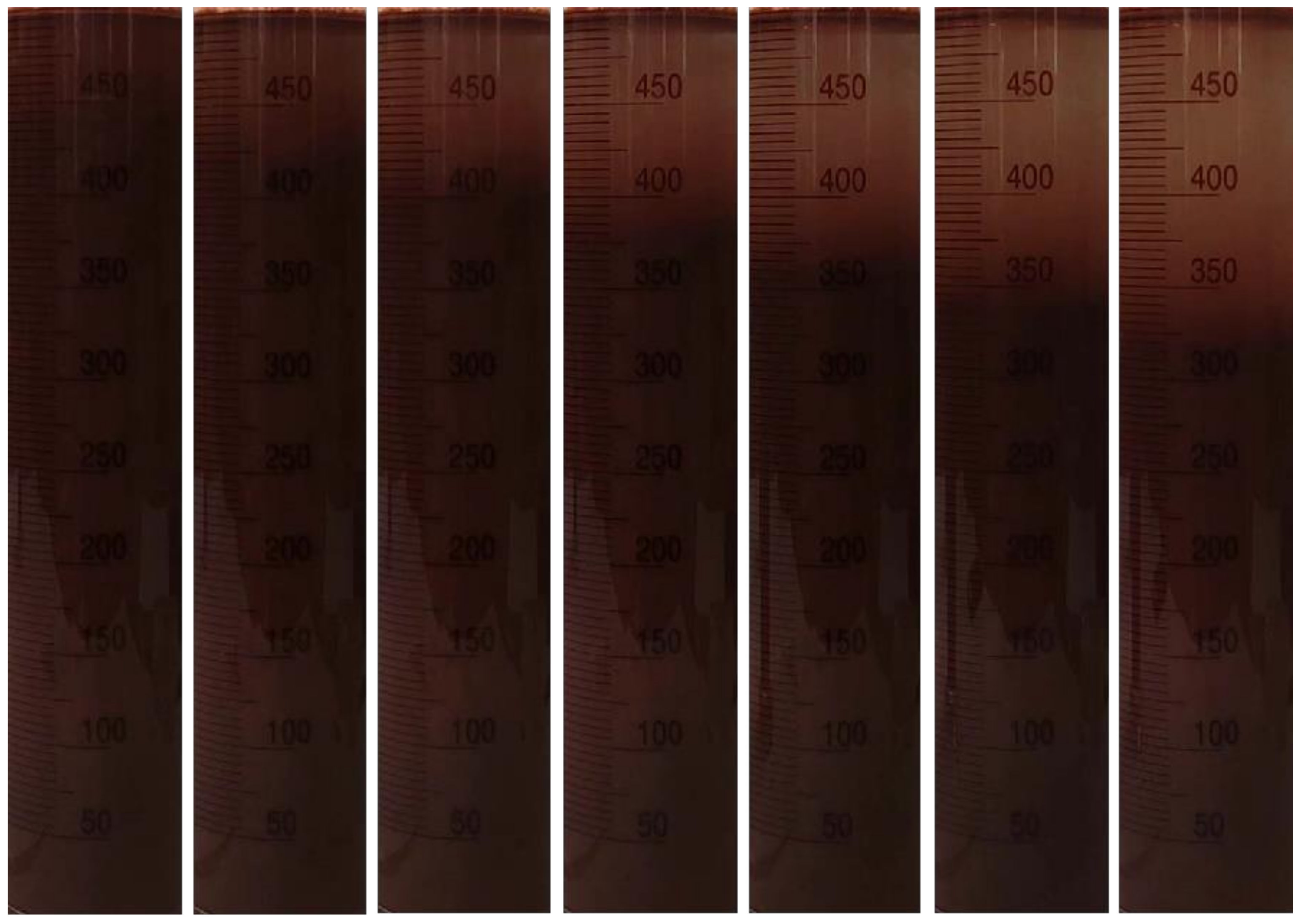
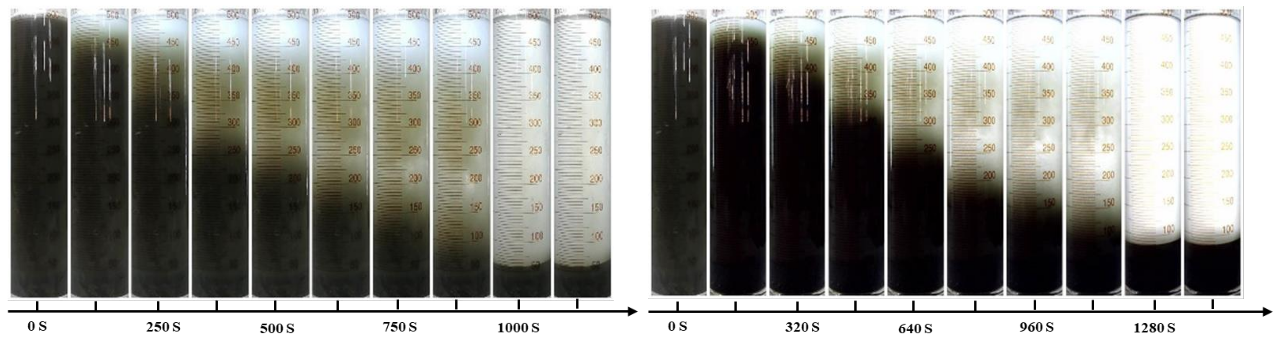
• Import high-definition video of the tailing sedimentation process, and take a final stable image as the classification basis. The upper liquid is generally regarded as the overflow water, which contains tailing particles that cannot settle.
• Import the stable grayscale image. The image is processed into an m × n two-dimensional matrix, where each element in the matrix represents the meeting value of the corresponding pixel, and the gray value varies from 0 (black) to 255 (white).
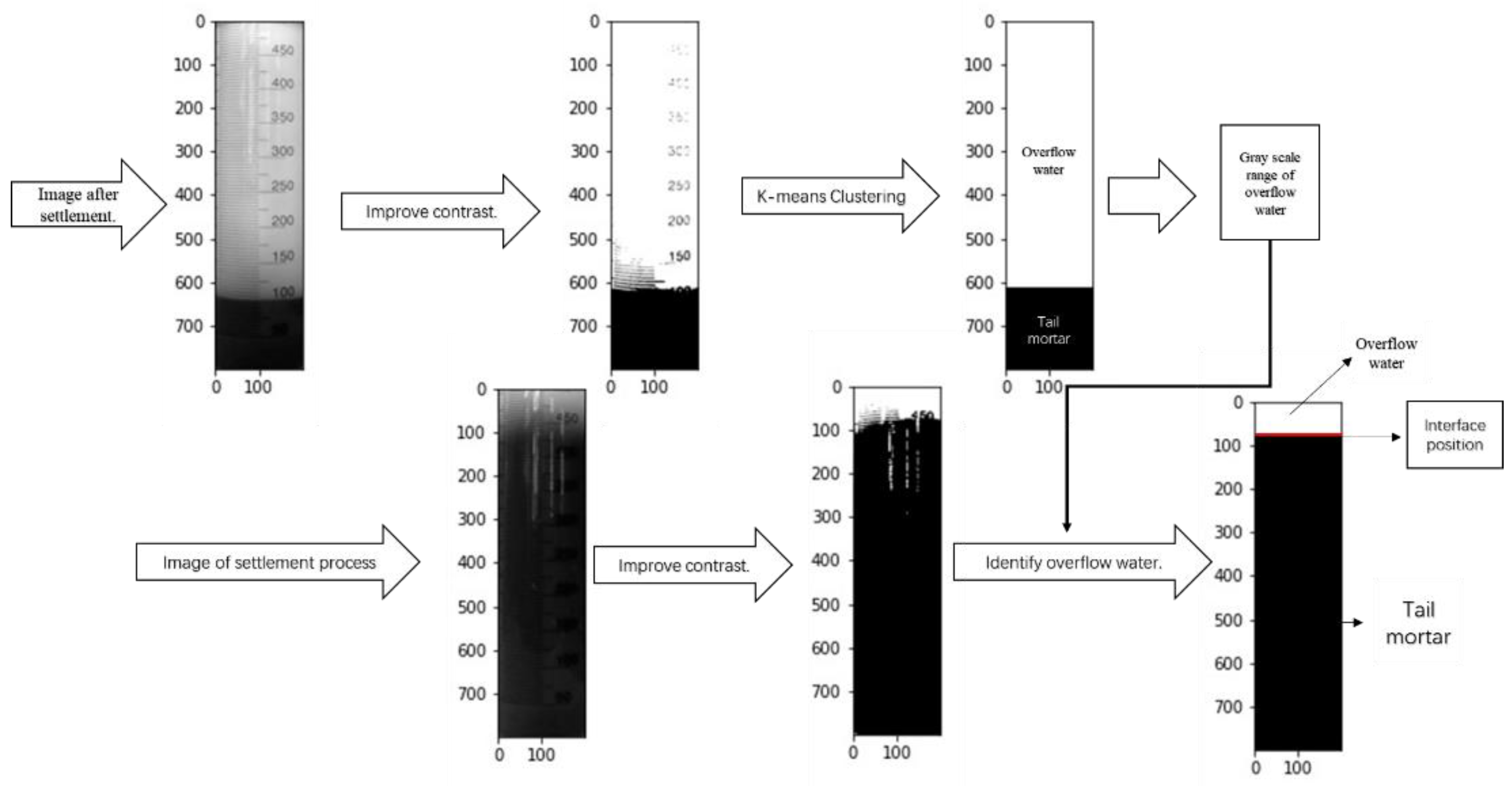
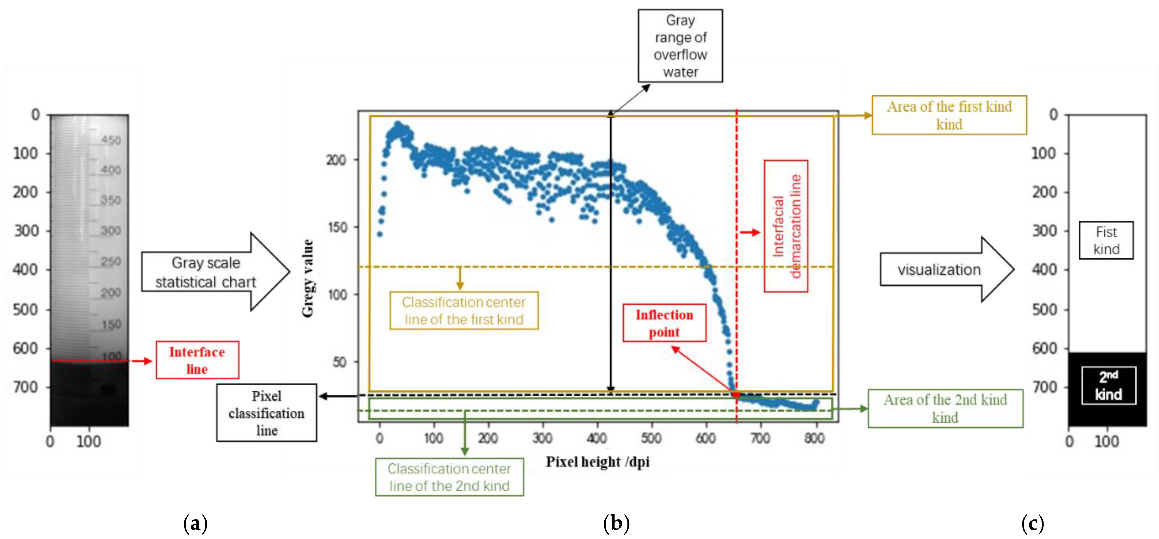
• Using the histogram equalization method, the contrast is improved, and the image is enhanced, so that the objects and shapes in the image are more prominent. Each row of pixels in the image is regarded as an object for K-means clustering analysis, and all objects are divided into two groups, namely the overflow water group and the tailings group. At the same time, center point A of the classification, that is, the basis point of the classification, can be obtained. In the gray image, the smaller the gray value, the darker the image; the more solid particles contained in the tail mortar, the darker the image will be, so the range of the gray value from 255 to “a” indicates the gray range of the tail mortar that cannot settle, that is, the gray range of the overflow water group.
• Import the gray image in the process of settlement, and use histogram equalization to improve the contrast and enhance the image. Use the gray scale range of the overflow water group, obtained in Step 3, to identify the overflow water group in the image. Finally, the position of the solid–liquid interface is obtained, from which the settling velocity can be calculated.

The settling process of the tailings is affected by factors, such as the type of tailing, physical and mechanical properties, particle size, concentration, and flocculant, which will lead to drastic changes in the concentration and color of overflow water. Taking the gray scale range of the overflow water in a stable state as a reference, the deviation caused by the above reasons can be effectively avoided, and the accuracy of the settlement interface identification is better ensured.

3. Application Example

Taking the tailings from a copper mine as an example, unsupervised learning is used as the identification method to determine the settlement interface of tailings and calculate the settlement velocity. The mine tailings are small in terms of granularity, and the tailings of a vertical sand silo are used for a cement filling. The key technology lies in the rapid settlement of tailings. The realization of rapid settlement depends on the selection of tailing settlement parameters (feed concentration, flocculant, etc.), and the basis of the selection of settlement parameters is used to measure the settlement speed of tailing slurry at different concentrations.

3.1. Physical and Mechanical Properties of Tailings

The physical and mechanical properties of the mine tailings are shown in

Table 2. Physical properties of tailings.

Number of Tests	Mass (g)	Volume (mm3)	Apparent Density (t/m3)	Loose Density (t/m3)	Packing Compactness	Void Ratio
Test 1	53.76	20.40	2.64	1.39	-	-
Test 2	53.75	20.40	2.64	1.37	-	-
Test 3	56.61	21.39	2.65	1.38	-	-
Average	-	-	2.68	1.38	51.50%	48.50%

, and the gradation distribution of the tailings is shown in

Table 3. Gradation distribution of tailings.

Particle Size (μm)	Distribution (%)
250	1.79
185	19.27
97.5	21.37
61.5	23.90
43	7.70
34.5	6.37
30	19.61

. It can be seen from Table 3 that 19.61% of the total tailings are smaller than 500 mesh. The average particle size of the tailings is 87.22 μm, and the median particle size is 58 μm.

From

Table 4. Analysis results of mineral composition of tailings.

Mineral Name	Mineral Content (%)
Calcite	40–50
Mica	25–35
Fluorite	5–10
Dolomite	5–10
Amphibole	1–5

, showing the mineral composition analysis, it can be seen that the main components of the tailings are calcite and mica, accounting for 40–50% and 23–35%, respectively. The chemical properties of the tailings are relatively stable, and there is no chemical reaction with water. The PH of the tailings slurry is shown in

Table 5. PH value of tailing slurry with different concentrations.

Mass Concentration	PH
15%	7.15
20%	7.15
25%	7.15
30%	7.15
35%	7.16
40%	7.16

, The PH of the tailings slurry is about 7; the slurry is neutral, and the PH remains basically unchanged with the increase in concentration.

3.2. Experimental Study

The K-means unsupervised learning classification method can classify tailings and overflow water after settlement stabilization and distinguish them in images in order to judge the interface in the settlement process and calculate the settlement speed. Because of visual recognition, the influence of illumination on environmental variables is very important; therefore, the test device (shown in Figure 3) was designed.

The experimental device consists of a black box, a measuring cylinder, a light source, and a high-definition camera. The experiment is performed in the black box and is not affected by external light source to ensure that the influence of external light sources on visual recognition is minimized. The light source is a 300-mm-long LED strip. There are 30 SMD LED beads on the lamp belt. The luminous brightness of the beads is 300 LM, the power of the lamp belt is 7.2 W/m, the voltage is 3–3.2 V, and the luminous angle is 120°. The light source is located behind the measuring cylinder, 50 mm away from the measuring cylinder, which provides the illumination conditions for the experimental process. The experiment was recorded using a high-definition camera. The camera used a Canon EOS 200D optical viewfinder, The manufacturer is Japan Canon Company, manufactured in Oita Prefecture, Japan. and the photosensitive element is CMOS. When recording video, it uses the 1080P short film shooting mode, with the sensitivity of ISO100–ISO12800, and the automatic exposure function is turned off. The optical viewfinder is installed on a tripod, and its highest point is level with the center of the measuring cylinder. The distance between the optical viewfinder and the measuring cylinder is 100 mm, focusing on the measuring cylinder. After enough settling time, the black box is opened to obtain the image data taken using the high-definition camera.

Tailing settlement is not only affected by physical and mechanical properties and particle size distribution of tailings but also by the slurry concentration. Therefore, different concentrations of tailings, from 15% to 40%, were designed. The unsupervised learning method is compared with manual recognition to verify the accuracy of the unsupervised learning results.

3.3. Experimental Results and Analysis

Screenshots of the shooting results of the HD camera at certain time intervals are shown in Figure 4. In Figure 4, on the left, is the tailing slurry with mass concentration of 15%, and the axis is the interval time of each image; the time scale of the axis is 125 s. On the right is the tailing slurry with mass concentration of 20%; the time scale of several axes is 160 s.

It can be seen that the settling speed of particles is very fast in the early stage of the experiment, but it is difficult to manually determine the interface position due to the influence of fine particles. In the later stage, the settlement velocity decreases, the interface tends to be stable, and the interface position remains unchanged for a long period of time. Therefore, the gray scale interval of the overflow water can be obtained using the image after sedimentation stabilization.

The process of determining the gray range of the overflow water is shown in Figure 5. The grayscale mode is used to import the image after settlement, and the range of the grayscale values is [0, 255], as shown in Figure 5a. (In this example, the pixels of the image are adjusted to 800 × 200 dpi, and the more pixels there are, the higher the accuracy is, and the more computing resources are occupied.) In order to conveniently explain the principle of judging the gray value of overflow water, each row of pixels in the picture is averaged and expanded into a gray statistical chart, as shown in Figure 5b. Each row of pixels will be in different positions according to the average gray value, and its positions can be roughly divided into two categories. One is the point with a larger gray value, where the gray value is greater than 100 and is visually lighter in color. The other type is the point with a smaller gray value, with a gray value below 50, and the visual expression of the color is darker.

As can be seen from Figure 5b, there are obvious differences in the gray values at different heights. Because the imported image is a settled image, its interface is visible to the naked eye (as shown in Figure 5a). The gray value is discontinuous at the interface, and there is an inflection point (as shown in Figure 5b). The inflection point is the point where the gray value of the overflow water has the smallest (because the larger the gray value, the lighter the color, and the larger the gray value, the lower the concentration). Therefore, as long as the coordinates of the inflection point are obtained, the minimum gray value of the overflow water can be obtained (Assuming that the value is a, then, the interval [a, 255] is the gray range of the overflow water). With different concentrations and physical characteristics of tailing slurry, the gray image of the tailings after settlement is different. The only similarity is that they all have inflection points that can determine the gray value of the interface. That is to say, as long as gray value a of the inflection point is obtained in each video, the gray range of the overflow water [a, 255] can be determined, and the overflow water and the interface position of each image in the video can be judged based on this. Averaging the gray values of each row of pixels is only for convenience of explaining the principle and visualization of coordinates. In actual operations, the gray values of each row of pixels are represented by a 200-dimension matrix (hypersurface.) Therefore, the K-means clustering method is used to classify the gray values of each row. They are fully divided into two categories, as shown in Figure 5b. Each category has a center line (plane), which indicates that each element in the category has the shortest distance from the center line. The first category is the overflow water. As long as the classification center of the overflow water is determined, the minimum gray value of the overflow water can be obtained. In actual operations, the gray value boundary of the overflow water can be obtained through iterative comparison, etc. With the solution with water as medium, a larger gray value means clearer water, and the lower the slurry concentration, the range of the minimum gray value of the overflow water to 255 is the gray value range of the overflow water. It is important to point out that the gray value range of the overflow water is affected by the physical characteristics of the tailings, settling concentration, water quality, pH, etc., so, the gray value range of the overflow water only represents the range of the gray value of the overflow water of tailing slurry in this video, and it cannot be applied to other concentrations and other tailings.

Taking the gray scale range of the overflow water as the judging condition of the overflow water, we can determine the image area of the overflow water by introducing it into each frame of the settlement process. Because the settlement process is caused by gravity, the area of the overflow water must expand from the top to the bottom. Therefore, in each image, the part excluding the overflow water is regarded as part of the tailing slurry, and the dividing line between the overflow water and the tailing slurry on the pixel scale is the solid–liquid interface to be identified. Therefore, the interface of each frame of the images in the settlement process can be determined. Based on the above principle, the images of the interface changes over time under different concentrations are shown in Figure 6, and the calculated settlement speed is shown in

Table 6. Tailings settling velocity.

Mass Concentration (%)	Volume Concentration (%)	Sedimentation Rate (m/s)
15	5.68	8.333 × 10−4
20	7.86	7.658 × 10−4
25	10.21	6.982 × 10−4
30	12.76	6.270 × 10−4
35	15.52	6.091 × 10−4
40	18.54	5.466 × 10−4

.

As shown in Figure 6, the relationship between the height and time of the settlement interface, identified using the unsupervised learning method, agrees with the actual situation; that is, the settlement interface will gradually decrease with the passage of time, and after a certain period of settlement, the interface will remain stable and not decrease. Comparing the settling velocity of the tailing slurry at different concentrations, it can be seen that the settling velocity will decrease with the increase in tailings slurry concentration, and the decreasing range is smaller and smaller, which is also consistent with the relationship between the settling velocity and the concentration that was observed manually. After settlement, the interface height basically does not change.

Comparing the results of K-means unsupervised learning with those of manual recognition (taking a concentration of 15% as an example), as shown in Figure 7, we can clearly see the advantages of unsupervised learning: it can read the interface data that cannot be distinguished through manual recognition; that is, the data that cannot be recognized through manual recognition because the interface is not obvious at the beginning of the settlement process. Secondly, there is little difference between the results of K-means unsupervised learning and those of manual recognition, and the maximum error does not exceed 3%. Moreover, using K-means unsupervised learning to identify the settlement speed is very fast, and the identification process is completed in a few seconds (60 images), which saves a great deal of time compared with manual identification and, thus, greatly improves work efficiency.

4. Conclusions

Tailing settling velocity is important information to be obtained for filling slurry making and filling system optimization. Because of the small particle size of tailings, the interface is not obvious in the initial stage of sedimentation. Unsupervised learning can effectively avoid the subjectivity and randomness of settlement interface judgments and make more scientific, accurate, and evidence-based judgments.

• The identification model of the tailing settlement speed adopts the K-means unsupervised classification method to identify the stabilized settlement image and judge the gray value interval of the overflow water. By identifying the overflow water, the interface in the settlement process can be judged, and the settlement speed can be calculated. The model has the characteristics of a high recognition accuracy and high speed. Because of the unsupervised learning method, the recognition accuracy of the model is independent of the amount of learning data, and only stable images are needed for recognition and analysis. Moreover, the model has a wide range of applications and has a high recognition accuracy for the settlement interface of tailing mortar with different particle size distributions, physical and mechanical properties, and flocculant addition or not.
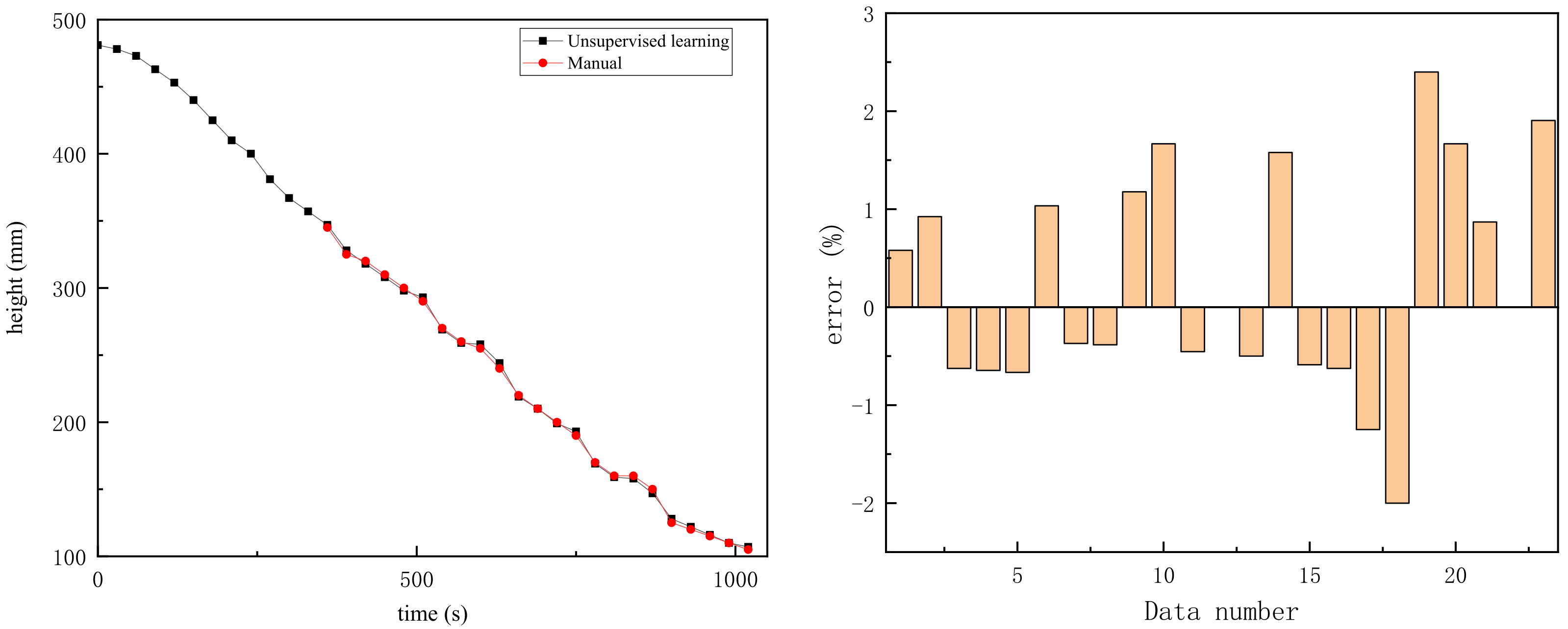
• Taking the tailing settlement of a copper mine as an example, the unsupervised learning model is applied to the tailing settlement process. Based on images of tailings at different concentrations in a final stable state, the interface position in the process of tailing settlement is identified, and the settlement speed of the tailings is obtained. The experimental results show that the model can identify the interface position, which cannot be distinguished manually, and gives the settlement velocity of the initial settlement. In addition, when the position of the interface can be determined, the accuracy of the model recognition is high, and the error rate is small.

The research results provide a new idea and reliable technical support for the determination of the settlement velocity of mine tailings and the optimization of parameters.

References

1. Wu, A.; Yang, Y.; Cheng, H.; Chen, S.; Han, Y. Development status and trend of paste technology in China. J. Eng. Sci. 2018, 40, 517–525. [Google Scholar]
2. Wu, A.; Wang, Y.; Wang, H. Present situation and trend of paste filling technology. Metal. Mine 2016, 7, 1–9. [Google Scholar]
3. Qiao, D.; Cheng, W.; Zhang, L.; Yao, W.; Wang, X.; Wang, H. Modern mining concept and filling mining. Sci. Eng. Nonferr. Met. 2011, 2, 7–14. [Google Scholar]
4. Rulyov, N.; Laskowski, J.S.; Concha, F. The use of ultra-flocculation in optimization of the experimental flocculation procedures. Physicochem. Probl. Miner. Proc. 2011, 1, 5–16. [Google Scholar]
5. Jiao, H.; Wu, A.; Wang, H.; Liu, X.; Yang, S.; Xiao, Y. Experiment study on the flocculation settlement characteristic of unclassified tailings. J. Beijing Univ. Sci. Technol. 2011, 33, 1437–1441. [Google Scholar] [CrossRef]
6. Zhang, Q.; Xie, S.; Zheng, J.; Wang, X. Study on settlement law of filling slurry and feasibility analysis of transportation. J. Chongqing Univ. 2011, 34, 105–107. [Google Scholar]
7. Shi, X.; Hu, H.; Du, X.; Li, M.; Wang, H. Experimental study on flocculation settlement of mortar liquid at the tail of vertical sand silo. Min. Metall. Eng. 2010, 30, 1–11. [Google Scholar]
8. Caifu, U.; Cuiping, L.; Bingheng, Y.; Gezhong, C. Effect of water reducer on rheological properties of fine tailings paste. Trans. Nonferr. Met. Soc. China 2021, 10–13, 1–17. [Google Scholar]
9. Wen, Z.; Yang, X.; Li, L.; Gao, Q.; Wang, Z. Selection and optimization of flocculation settlement parameters of whole mortar based on RSM-BBD. Trans. Nonferr. Met. Soc. China 2020, 30, 1437–1445. [Google Scholar]
10. Xi, W.; Chao, Y.; Qu, W.; Kun, G. Research on speech emotion recognition based on PCA-RF classification. Sci. Technol. Innov. 2021, 29, 91–93. [Google Scholar]
11. Wu, X.; Yan, D. Analysis and research on data dimension reduction methods. Res. Comput. Appl. 2009, 26, 2832–2835. [Google Scholar]
12. Elkin, M.; Niyogi, P. Laplacian Eigenmaps and Spectral Techniques for Embedding and Clustering. Adv. Neural Inf. Process. Syst. 2001, 14, 585–591. [Google Scholar]
13. Yuting, K.; Fuxiang, T.; Xin, Z.; Zhenghang, Z.; Lu, B.; Yurong, Q. Review of K-means Algorithm Optimization Based on Differential Privacy. Comput. Sci. 2021, 1–21. [Google Scholar] [CrossRef]
14. Lu, X.; Xu, L.; Zhang, M. Security hierarchical virtual network mapping method based on clustering. Telecommun. Sci. 2021, 37, 112–117. [Google Scholar]
15. Ji, Q.; Sun, Y.; Hu, Y.; Yin, B. A survey of deep clustering algorithms. J. Beijing Univ. Technol. 2021, 47, 912–924. [Google Scholar]
16. Deng, X.; Yu, L. Summary of Deep Clustering Algorithms. Commun. Technol. 2021, 54, 1807–1814. [Google Scholar]
17. Yin, F.; Cao, X.; Qi, X. Summary of recommendation algorithms based on clustering. J. Southwest Minzu Univ. 2021, 47, 303–309. [Google Scholar]
18. Zhou, Y.; Ren, Q.; Niu, H. A summary of research on training sample data selection methods. Comput. Sci. 2020, 47, 402–408. [Google Scholar]
Figure 1. Schematic diagram of the settlement process.
Metals 11 01903 g001
Figure 2. Principle of unsupervised learning to identify settling velocity of tailings.
Metals 11 01903 g002
Figure 3. Schematic diagram of experiment device.
Metals 11 01903 g003
Figure 4. Settlement experiment: (left) mass concentration 15%, (right) mass concentration 20%.
Metals 11 01903 g004
Figure 5. Determination of gray scale range of overflow water. (a) original image; (b) gray statistical chart; (c) visualization of classification results.
Metals 11 01903 g005
Figure 6. Unsupervised learning recognition result of interface settlement.
Metals 11 01903 g006
Figure 7. Comparison between the unsupervised learning recognition results and the manual recognition results.
Metals 11 01903 g007