
Dispatch Optimization Model for Haulage Equipment between Stopes Based on Mine Short-Term Resource Planning

 ,
, 
Abstract
:1. Introduction
1.1. Terms and Concepts
1.2. Dataset
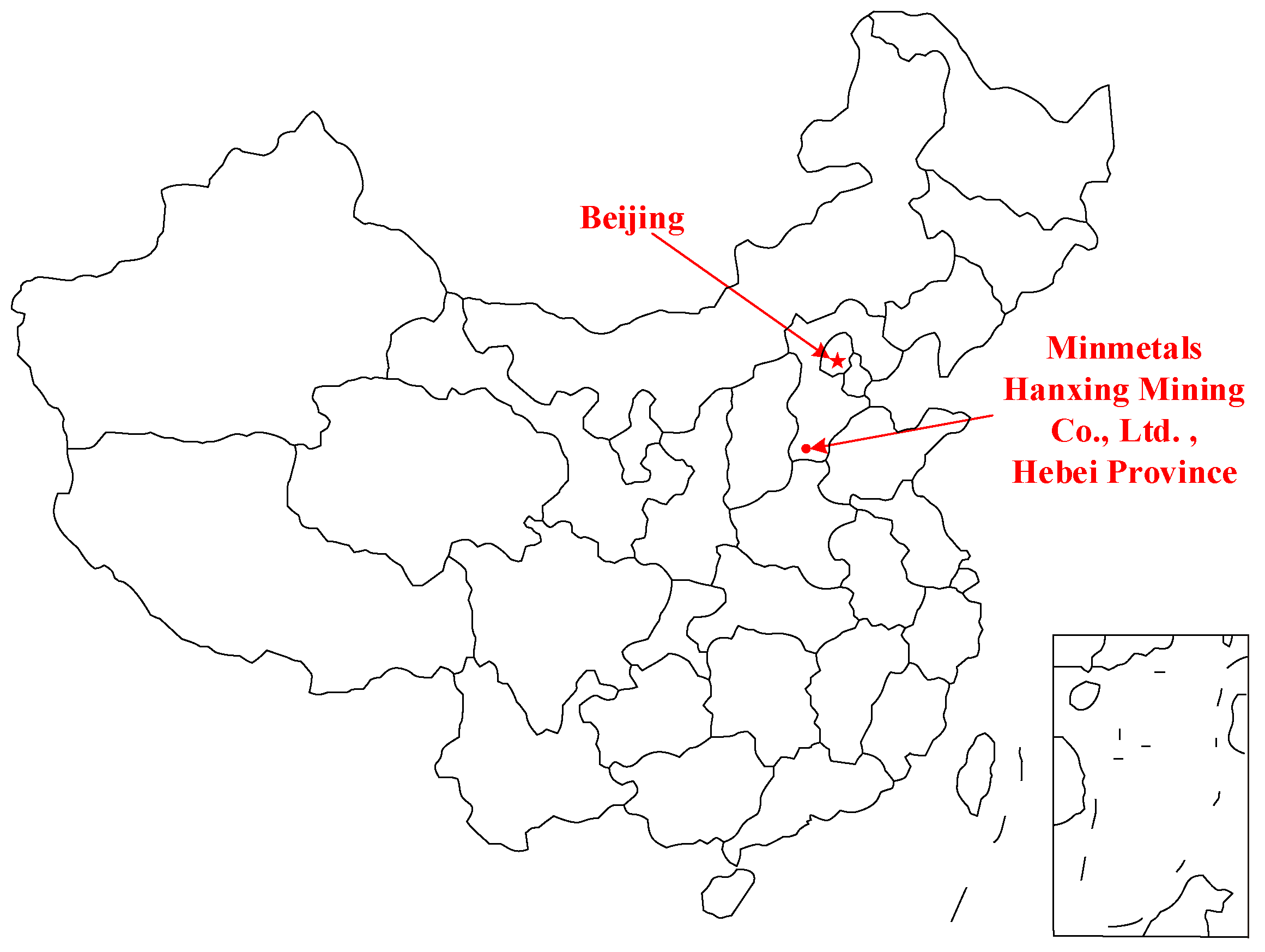
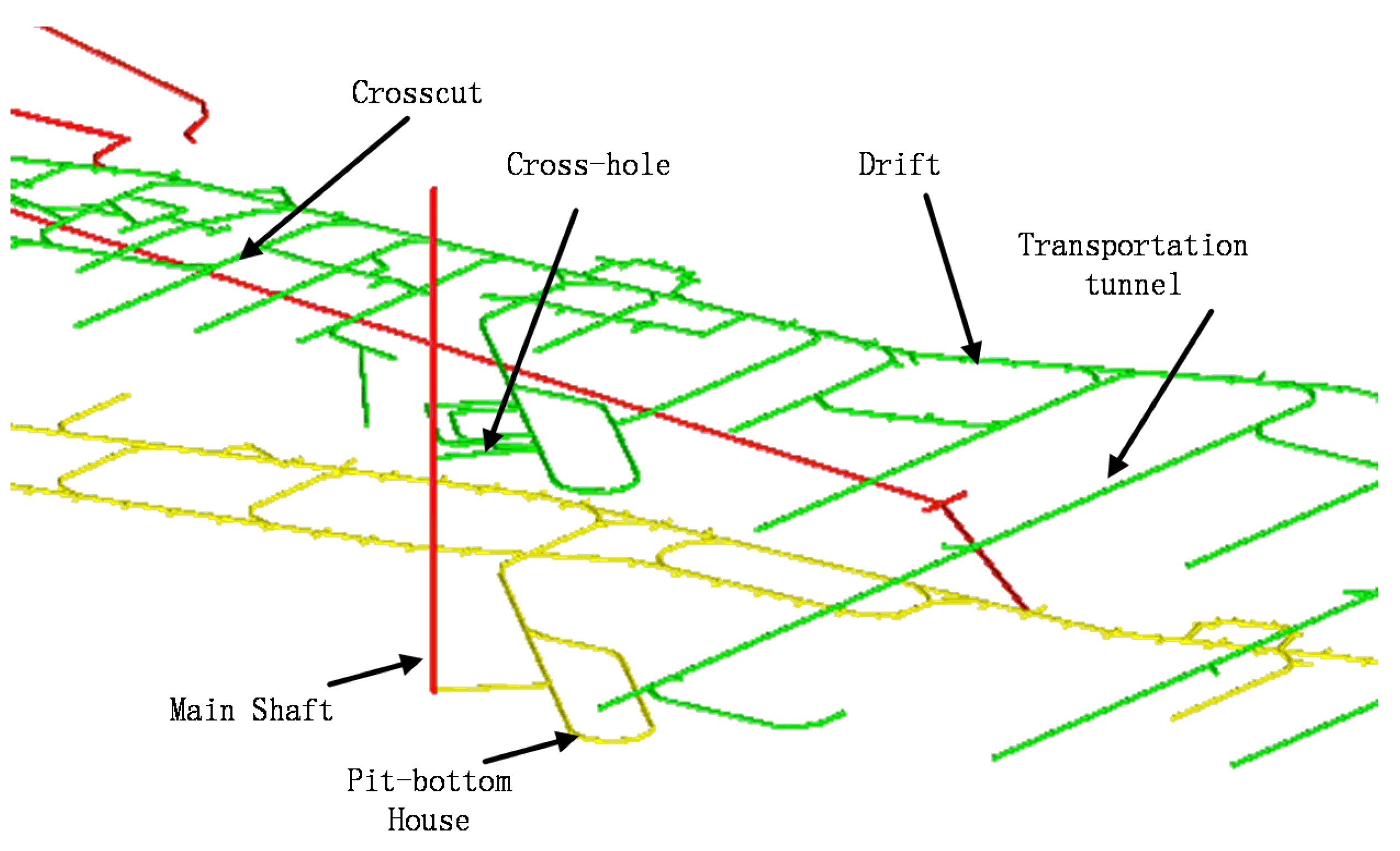
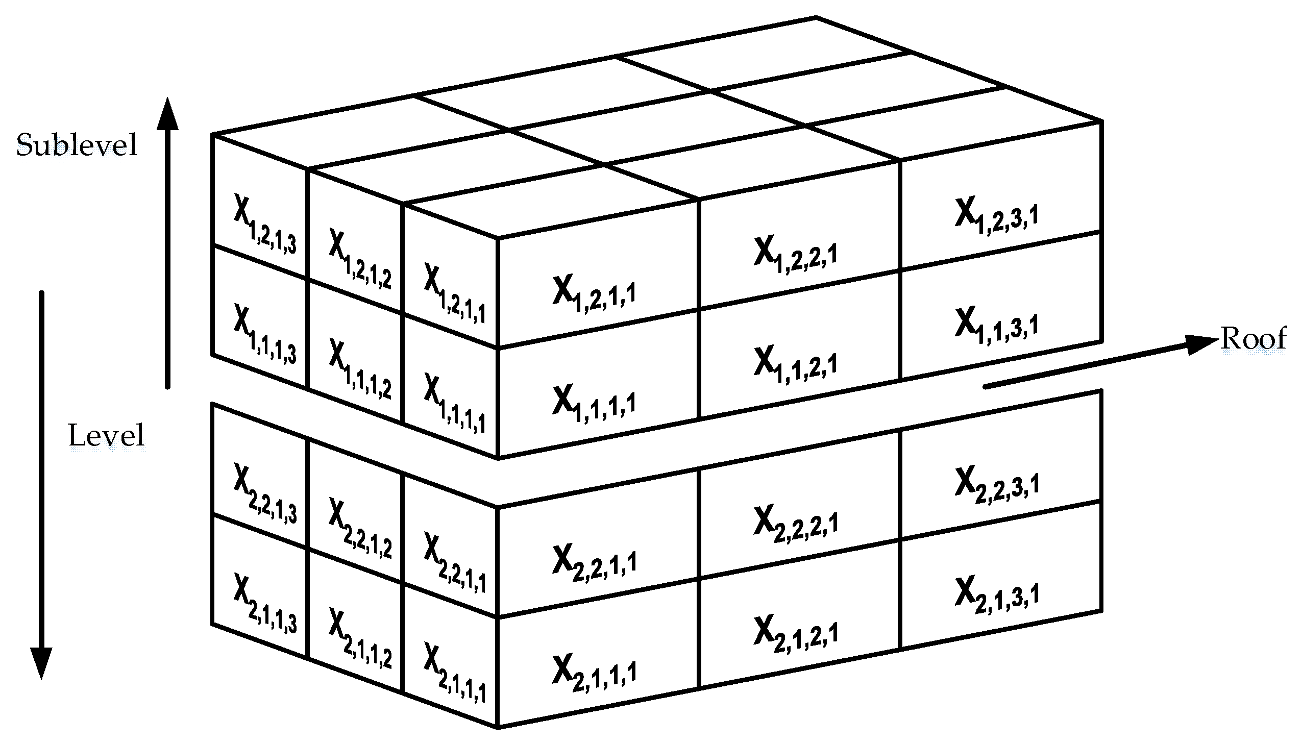
1.2.1. Mine Layout
1.2.2. Mining Methods
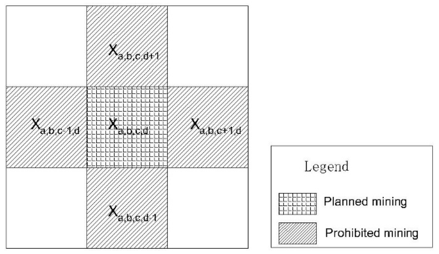
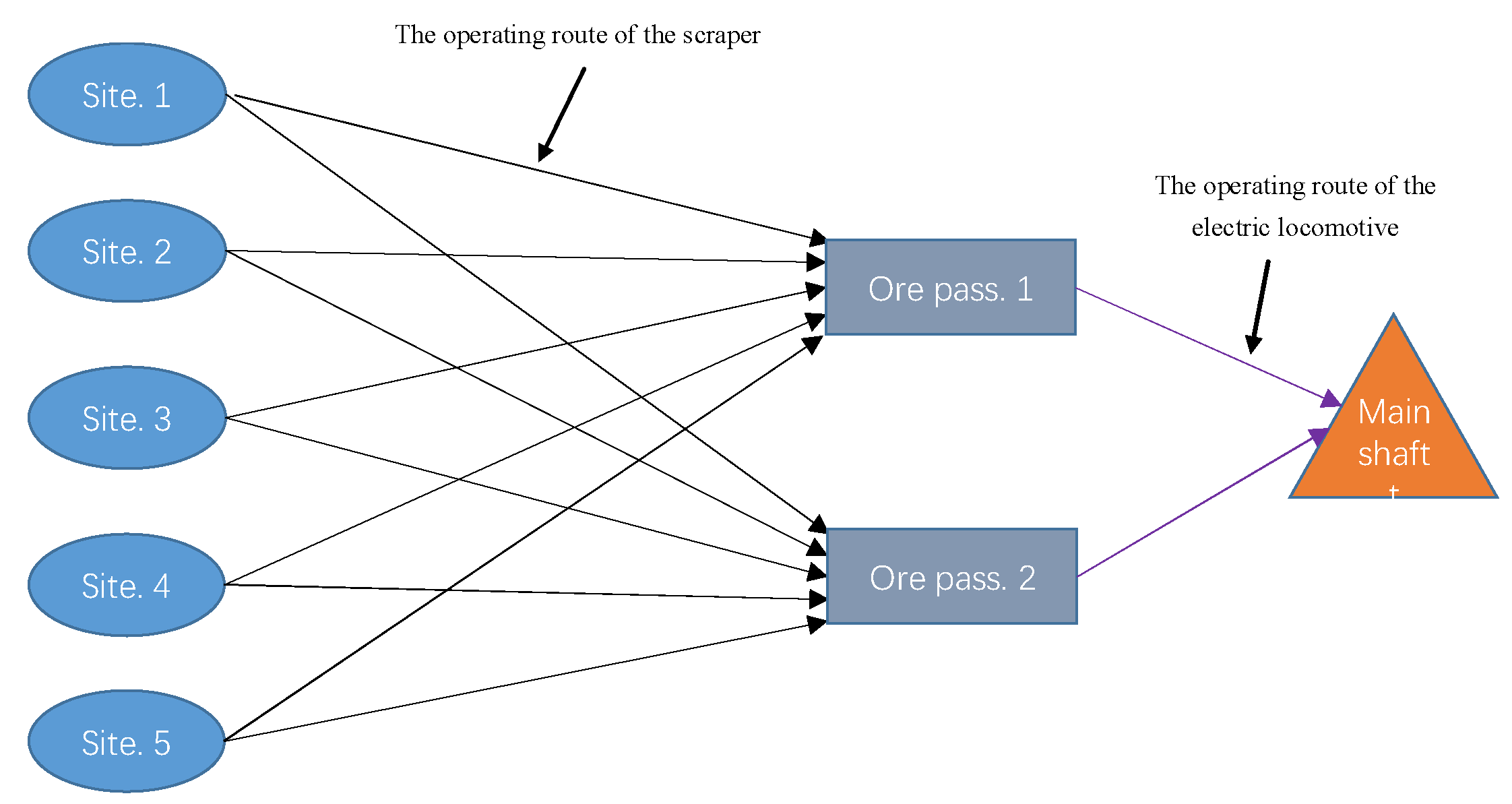
1.2.3. Spatial Relations
1.2.4. Haulage Equipment
2. Relevant Literature
2.1. Short-Term Resource Planning
2.2. Haulage Equipment Dispatch Planning
3. Model
3.1. Model of Short-Term Resource Planning
3.1.1. Sets
3.1.2. Parameters
3.1.3. Variables
3.1.4. Objective
3.1.5. Constraints
3.2. Haulage Equipment Dispatch Plan Model
3.2.1. Sets
3.2.2. Parameters
3.2.3. Variables
3.2.4. Objective
3.2.5. Constraints
4. Optimization Algorithm
4.1. Improved Artificial Bee Colony Optimization Algorithm
- (1)
- Determine the fitness value of the objective function and initialize the parameters, including the nectar population N, the maximum evolutionary generation t, and the custom generation limit;
- (2)
- The coding rules of the nectar source location, the nectar source population adopts binary coding are expressed as where m represents the sum of all variable elements of a single individual;
- (3)
- Initialize the nectar population, find a feasible solution according to the constraints of the optimization model, and randomly generate feasible solutions in the surrounding area of the feasible solution. All the generated feasible solutions form the initial nectar population;
- (4)
- Calculate the fitness value of the initial nectar source population, compare the fitness value of the current population, record the best individual value in the current population, and position the honeybees at the half of the nectar source in the population where the fitness value is better. The number of following bees is the same as the number of picking bees;
- (5)
- Picking bees are used to search the neighborhood at the current nectar source location. When the binary code of discrete variables is used, the neighborhood search becomes a value change 0 and 1. After the value is changed, it is judged whether it satisfies the constraint condition. If the constraint condition is not met, the variable is reselected near the value of the variable for transformation until the constraint condition is met, at which point, it can be used as a new nectar location. Then, calculate the fitness value and compare the fitness value of the new nectar source with the original nectar source. If the nectar source quality of the new nectar source is better, replace the original location with the new nectar source to update the nectar source population;
- (6)
- Compare the fitness value of the current population. Compare the current optimal individual with the recorded optimal individual, if it is better than the recorded optimal individual, replace it; otherwise, replace the recorded optimal individual back to the original one. Then, continue subsequent operations at the location;
- (7)
- According to the roulette selection method which is following bees choose a better position in the current nectar population and go through the neighborhood search method of step (5) and generate a new nectar source location around this location. Then, the following bee calculates the fitness value, compares the fitness value of the new nectar source with the original nectar source, selects the best to form a new nectar source population, and proceeds to step (6);
- (8)
- Determine whether part of the nectar source in the current nectar source population meets the abandonment condition. If a nectar source has not been replaced after the limit generation neighborhood search, then go to step (9), otherwise go to step (10);
- (9)
- If the nectar source is the best nectar source in the current population, do not abandon it; otherwise, the current nectar source is abandoned, and the picking or following bees at the current nectar source location become the scout bees. The nectar source randomly changes its position to form a new nectar source and updates the nectar source population;
- (10)
- Judge whether the end condition is reached, if the maximum number of iterations is not reached, the current nectar source population is used as the initial nectar source population, and steps (5), (6), (7), (8), and (9) are repeated. If the maximum evolutionary generation is reached, the optimal nectar source position in the current population is considered to be the optimal solution.
4.2. Non-Dominated Sorting Genetic Algorithm (NSGA-III)
- (1)
- Initialization parameters. The maximum evolutionary generation is the reference point size is H, the population size is N + 1, the crossover and mutation rates are and , respectively, and the evolutionary generation is t, which is set as 0.
- (2)
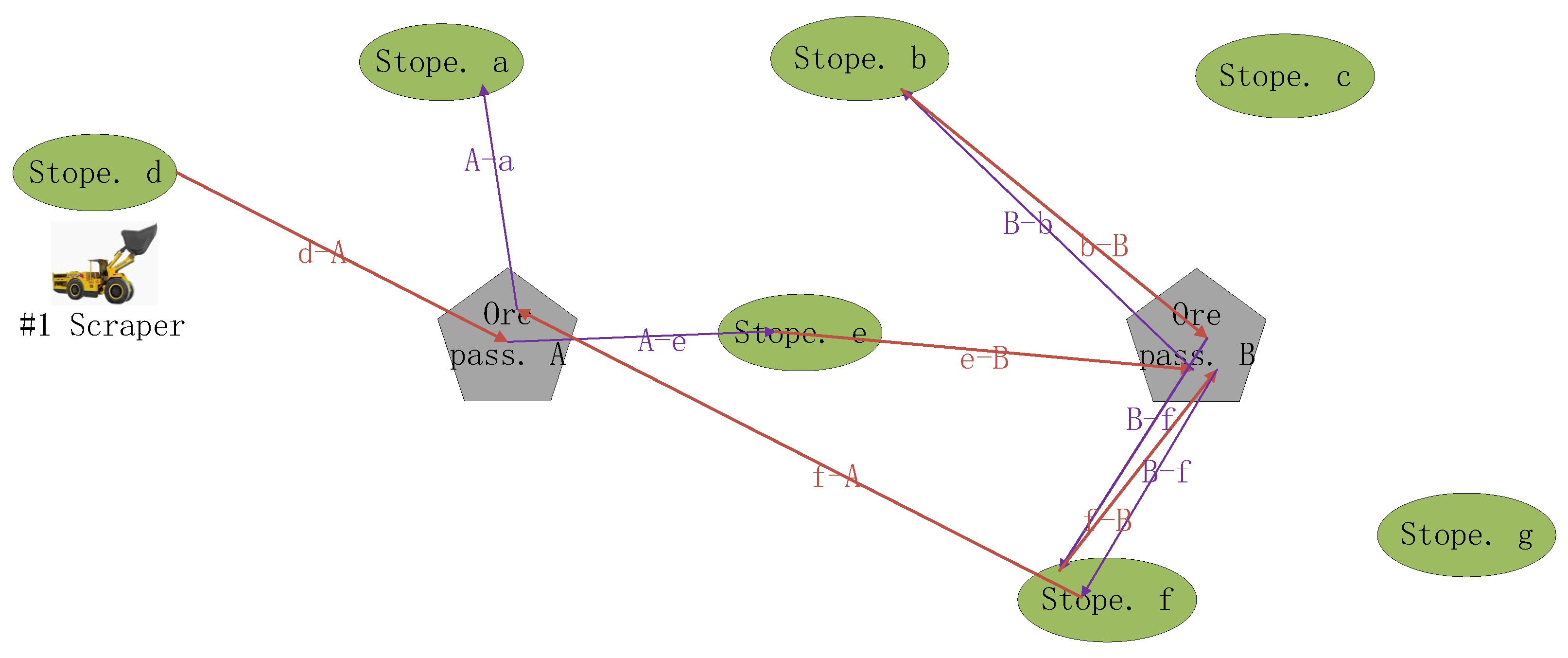
- Initialize the population. The scale is N. Each individual in the population consists of N+M chromosomes. The individual chromosomes are independent of each other. The maximum and minimum lengths of chromosomes are set. The length of each chromosome is randomly generated between the maximum and minimum values. The chromosomes are coded using characters, with lowercase for stopes, capital letters for ore passes, and the letter ‘Z’ for the main shaft. For example: represents the operating route of a scraper, while represents the operating route of an electric locomotive.
- (3)
- Determine the objective function. The Pareto ranking hierarchical comparison method is used for multiple objective functions.
- (4)
- Using rapid non-dominated sorting based on Pareto dominance, divide the current population into several dominance layers, select the best individuals in the first dominance layer based on the reference point-based constraint dominance relationship method, and extract them as a single population that does not participate in genetic manipulation. Then, subpopulation is generated through the crossover, mutation, and breaking of the genetic algorithm, with a scale of N. Crossover: randomly select chromosomes of the same nature for different individuals in the population to cross over random gene positions. Mutation: Chromosomal genetic properties mutate at random. Breaking: Each chromosome randomly chooses whether to perform the break operation, if so, cut two genes to the last position of the chromosome. The progeny population is generated through the operation sequence of crossover, mutation, and breaking.
- (5)
- Combine the offspring population and the parent population to form the population, use the non-dominated sort based on Pareto dominance to divide into several different non-dominated layers, and select N higher-level individuals as the next parent population. Individuals in the same level are selected using a reference point-based constraint dominance relationship method, also the best individual in the first dominance level of the parent population is selected using the same method.
- (6)
- Compare and select the optimal individual produced by the t + 1 generation with the optimal individual of the t generation. Use the method based on the reference point to select the superior individual among the two adjacent generations of optimal individuals. If the optimal individual of the t + 1 generation is superior, it will be placed in a separate population, and the original t generation optimal individual will be placed in t, where the best individual of the t + 1 generation is located, and form a new parent group.
- (7)
- Judge whether the parent population meets the termination conditions. If not, then t = t + 1, repeat steps (4), (5), and (6). If the termination conditions are met, then output the best individual.
5. Computational Study
5.1. Optimization Results
5.1.1. Resource Plan
5.1.2. Haulage Equipment Dispatch Plan
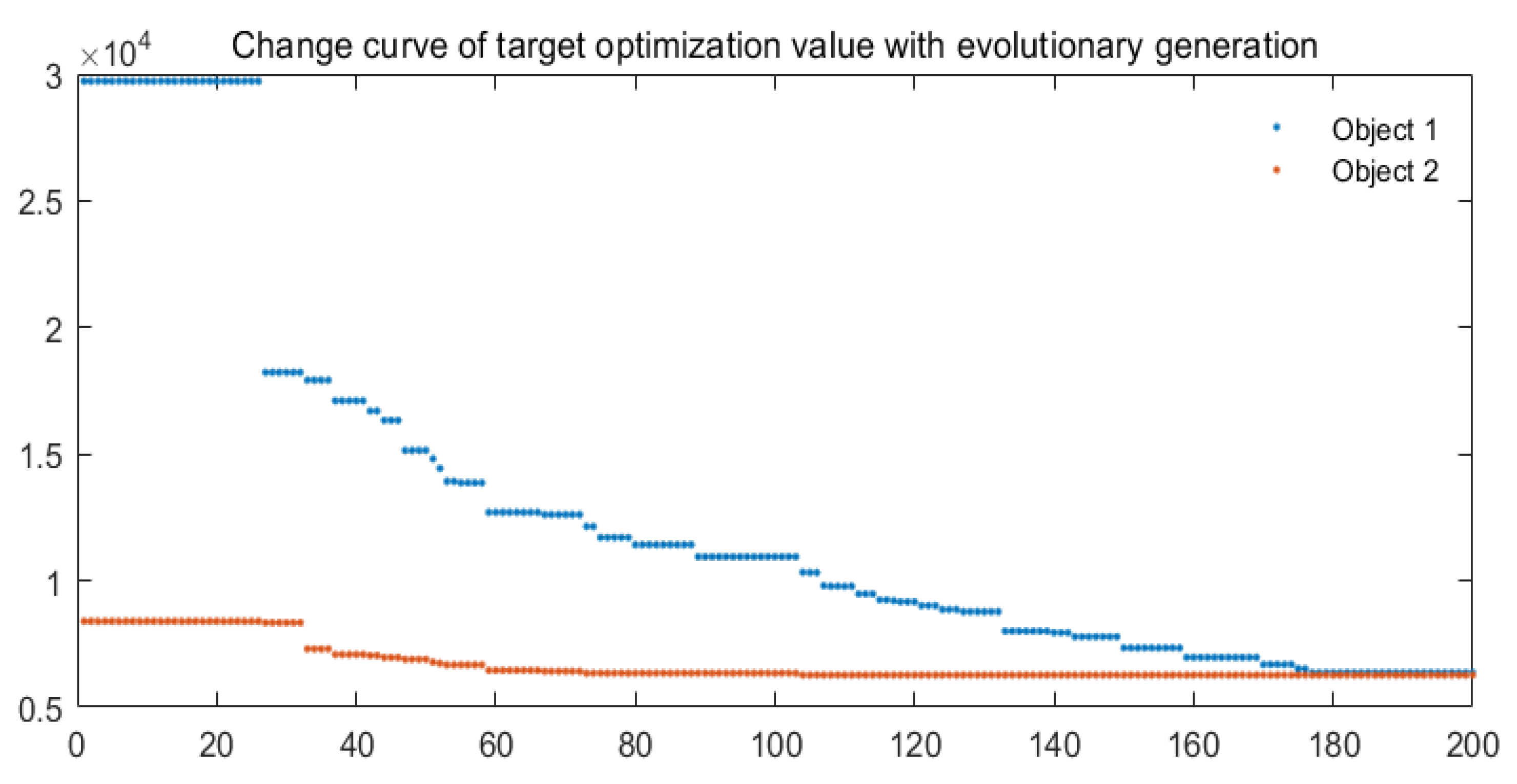
5.2. Result Analysis
6. Discussion
7. Conclusions
Author Contributions
Funding
Data Availability Statement
Acknowledgments
Conflicts of Interest
References
- Topal, E. Early start and late start algorithms to improve the solution time for long-term underground mine production scheduling. J. South. Afr. Inst. Min. Metall. 2008, 108, 99–107. [Google Scholar]
- Sandanayake, D.S.S.; Topal, E.; Ali Asad, M.W. A heuristic approach to optimal design of an underground mine stope layout. Appl. Soft Comput. 2015, 30, 595–603. [Google Scholar] [CrossRef]
- Wu, H.; Li, J. Open-pit Mine Production Planning: The Current, Problem& Strategies. Met. Mine 2005, 4, 4–6+42. [Google Scholar]
- Newman, A.M.; Rubio, E.; Caro, R.; Weintraub, A.; Eurek, K. A Review of Operations Research in Mine Planning. Interfaces 2010, 40, 222–245. [Google Scholar] [CrossRef] [Green Version]
- Zhan, K. Development trend of trackless mining equipment in underground metal mines. Min. Technol. 2006, 3, 34–38. [Google Scholar]
- Yi, X. Development Trend of Trackless Equipment in Mines in my country. Min. Equip. 2019, 1, 10–15. [Google Scholar]
- Li, Y.; Tong, G. General situation of the development of mine production planning method. Met. Mine 1994, 12, 11–16. [Google Scholar]
- Ming, J.; Li, G.; Hu, N. Optimization of Production Planning for Underground Metal Mines Based on Market. J. Univ. Sci. Technol. Beijing 2013, 35, 1215–1220. [Google Scholar]
- Nehring, M.; Topal, E.; Kizil, M.; Knights, P. Integrated short- and medium-term underground mine production scheduling. J. South. Afr. Inst. Min. Metall. 2012, 112, 365–378. [Google Scholar]
- O’sullivan, D.; Newman, A. Optimisation-based heuristics for underground mine scheduling. Eur. J. Oper. Res. 2015, 241, 248–259. [Google Scholar] [CrossRef]
- Zhou, K.; Gu, D. Optimization of Stoping Sequence in Underground Mining by Using Genetic Algorithm Method. China Min. Mag. 2001, 5, 52–56. [Google Scholar]
- Hou, J.; Hu, N.; Li, G.; Ma, Z.; Li, D.; Gong, J. Dynamic Optimization of Production Plans for Multi-Metal Underground Mines. Chin. J. Eng. 2016, 38, 453–460. [Google Scholar]
- Foroughi, S.; Hamidi, J.K.; Monjezi, M.; Nehring, M. The integrated optimization of underground stope layout designing and production scheduling incorporating a non-dominated sorting genetic algorithm (NSGA-II). Resour. Policy 2019, 63, 101408. [Google Scholar] [CrossRef]
- Gligoric, Z.; Gligoric, M.; Dimitrijevic, B.; Grozdanovic, I.; Milutinovic, A.; Ganic, A.; Gojkovic, Z. Model of room and pillar production planning in small scale underground mines with metal price and operating cost uncertainty. Resour. Policy 2020, 65, 101235. [Google Scholar] [CrossRef]
- Jiang, C.; Peng, P.; Wang, L. 3D Visualization Production Planning in Underground Ming Based on Simulating Technology. China Min. Mag. 2015, 24, 152–156. [Google Scholar]
- Liu, D.; Wang, L.; Chen, X.; Zhong, D.; Xu, Z. Study on Multi Objective Optimization and Application of Medium and Long Term Plan for Underground Mine. Gold Sci. Technol. 2018, 26, 228–233. [Google Scholar]
- Sarin, S.C.; West-Hansen, J. The long-term mine production scheduling problem. IIE Trans. 2005, 37, 109–121. [Google Scholar] [CrossRef]
- Newman, A.M.; Kuchta, M. Using aggregation to optimize long-term production planning at an underground mine. Eur. J. Oper. Res. 2007, 176, 1205–1218. [Google Scholar] [CrossRef]
- Riff, M.-C.; Otto, E.; Bonnaire, X. A New Strategy Based on GRASP to Solve a Macro Mine Planning. In Proceedings of the International Symposium on Foundations of Intelligent Systems, Prague, Czech Republic, 14–17 September 2009; pp. 483–492. [Google Scholar]
- Little, J.; Knights, P.; Topal, E. Integrated optimization of underground mine design and scheduling. J. South. Afr. Inst. Min. Metall. 2012, 113, 775–785. [Google Scholar]
- Mousavi, A.; Sellers, E. Optimisation of production planning for an innovative hybrid underground mining method. Resour. Policy 2019, 62, 184–192. [Google Scholar] [CrossRef]
- Campeau, L.-P.; Gamache, M. Short-term planning optimization model for underground mines. Comput. Oper. Res. 2020, 115, 104642. [Google Scholar] [CrossRef]
- Gligoric, Z.; Beljic, C.; Gluscevic, B.; Cvijovic, C. Underground Lead-Zinc Mine Production Planning Using Fuzzy Stochastic Inventory Policy. Arch. Min. Sci. 2015, 60, 73–92. [Google Scholar]
- Gamache, M.; Grimard, R.; Cohen, P. A shortest-path algorithm for solving the fleet management problem in underground mines. Eur. J. Oper. Res. 2005, 166, 497–506. [Google Scholar] [CrossRef]
- Saayman, P.; Craig, I.K.; Camisani-Calzolari, F.R. Optimization of an autonomous vehicle dispatch system in an underground mine. J. South Afr. Inst. Min. Metall. 2006, 106, 77–86. [Google Scholar]
- Nehring, M.; Topal, E.; Little, J. A new mathematical programming model for production schedule optimization in underground mining operations. J. South. Afr. Inst. Min. Metall. 2010, 110, 437–446. [Google Scholar]
- Sun, Y.; Lian, M. Research on Vehicle Routing and Scheduling Problems Based on Improved ACA in Underground Mine. Met. Min. 2010, 2, 51–54. [Google Scholar]
- Åstrand, M.; Johansson, M.; Zanarini, A. Underground Mine Scheduling of Mobile Machines using Constraint Programming and Large Neighborhood Search. Comput. Oper. Res. 2020, 123, 105036. [Google Scholar] [CrossRef]


| Number | Result | Total Storage/t | Remaining Storage/t | Grade/% |
|---|---|---|---|---|
| (1, 1, 4, 3) | 1 | 2883.92 | 2883.92 | 24.03 |
| (1, 1, 8, 3) | 1 | 2951.56 | 2951.56 | 61.74 |
| (1, 1, 11, 3) | 1 | 2631.26 | 2631.26 | 44.26 |
| (1, 1, 1, 2) | 1 | 2951.37 | 2951.37 | 36.46 |
| (1, 1, 6, 2) | 1 | 2601.16 | 2601.16 | 49.15 |
| (1, 1, 9, 1) | 1 | 2667.56 | 2667.56 | 49.28 |
| (1, 1, 12, 1) | 1 | 2916.49 | 2916.49 | 56.74 |
| (2, 1, 1, 3) | 1 | 2643.29 | 2643.29 | 35.77 |
| (2, 1, 4, 3) | 1 | 2708.67 | 2708.67 | 42.90 |
| (2, 1, 10, 3) | 1 | 2947.29 | 2947.29 | 31.48 |
| (2, 1, 2, 1) | 1 | 2938.19 | 2938.19 | 52.25 |
| (2, 1, 5, 1) | 1 | 2646.24 | 2646.24 | 54.64 |
| (2, 1, 8, 1) | 1 | 2951.56 | 2951.56 | 61.74 |
| (2, 1, 11, 1) | 1 | 2969.06 | 2969.06 | 44.26 |
| (2, 1, 7, 3) | 1 | 2671.67 | 2671.67 | 48.00 |
| Others | 0 | / | / | / |
| Ore Pass | Stope/(Number) | ||||||
|---|---|---|---|---|---|---|---|
| a | b | c | d | e | f | g | |
| (1, 1, 4, 3) | (1, 1, 8, 3) | (1, 1, 11, 3) | (1, 1, 1, 2) | (1, 1, 6, 2) | (1, 1, 9, 1) | (1, 1, 12, 1) | |
| A | 75.5 | 149.3 | 179.2 | 97.8 | 100.5 | 145.6 | 210.3 |
| B | 154.2 | 85.6 | 96.2 | 205.2 | 137.3 | 79.7 | 100.5 |
| Ore Pass | Stope/(Number) | ||||||
|---|---|---|---|---|---|---|---|
| a | b | c | d | e | f | g | |
| (1, 1, 4, 3) | (1, 1, 8, 3) | (1, 1, 11, 3) | (1, 1, 1, 2) | (1, 1, 6, 2) | (1, 1, 9, 1) | (1, 1, 12, 1) | |
| A | 52.49 | 105.7 | 147.5 | 64.5 | 67.8 | 104.3 | 172.6 |
| B | 110.7 | 57.5 | 61.3 | 144.2 | 84.6 | 54.0 | 68.2 |
| Ore Pass | Stope/(Number) | |||||||
|---|---|---|---|---|---|---|---|---|
| s | t | u | v | w | x | y | z | |
| (2, 1, 1, 3) | (2, 1, 4, 3) | (2, 1, 7, 3) | (2, 1, 10, 3) | (2, 1, 2, 1) | (2, 1, 5, 1) | (2, 1, 8, 1) | (2, 1, 11, 1) | |
| C | 87.3 | 86.7 | 144.7 | 173.7 | 91.8 | 114.7 | 152.9 | 177.4 |
| D | 157.6 | 133.3 | 92.3 | 132.7 | 145.7 | 87.2 | 67.1 | 134.7 |
| E | 214.7 | 195.7 | 113.8 | 56.4 | 215.3 | 187.3 | 105.4 | 80.5 |
| Ore Pass | Stope/(Number) | |||||||
|---|---|---|---|---|---|---|---|---|
| s | t | u | v | w | x | y | z | |
| (2, 1, 1, 3) | (2, 1, 4, 3) | (2, 1, 7, 3) | (2, 1, 10, 3) | (2, 1, 2, 1) | (2, 1, 5, 1) | (2, 1, 8, 1) | (2, 1, 11, 1) | |
| C | 54.5 | 54.2 | 106.7 | 129.8 | 56.3 | 73.2 | 111.4 | 132.3 |
| D | 110.3 | 89.6 | 56.7 | 90.5 | 107.3 | 55.1 | 43.8 | 92.3 |
| E | 162.3 | 141.4 | 72.7 | 34.3 | 160.9 | 137.9 | 69.6 | 51.7 |
| Main Shaft | Ore Pass | ||||
|---|---|---|---|---|---|
| A | B | C | D | E | |
| Z | 900 | 963 | 935 | 973 | 892 |
| Main Shaft | Ore Pass | ||||
|---|---|---|---|---|---|
| A | B | C | D | E | |
| Z | 725 | 772 | 741 | 694 | 711 |
| Ore Pass | Stope | ||||||||||||||
|---|---|---|---|---|---|---|---|---|---|---|---|---|---|---|---|
| a | b | c | d | e | f | g | s | t | u | v | w | x | y | z | |
| A | 19 | 20 | 26 | 20 | 26 | 30 | 35 | / | / | / | / | / | / | / | / |
| B | 21 | 13 | 16 | 28 | 15 | 18 | 15 | / | / | / | / | / | / | / | / |
| C | / | / | / | / | / | / | / | 9 | 14 | 7 | 17 | 9 | 16 | 19 | 17 |
| D | / | / | / | / | / | / | / | 13 | 9 | 6 | 13 | 8 | 12 | 6 | 7 |
| E | / | / | / | / | / | / | / | 14 | 4 | 10 | 6 | 15 | 13 | 7 | 6 |
| Main Shaft | Ore Pass | ||||
|---|---|---|---|---|---|
| A | B | C | D | E | |
| Z | 6 | 7 | 6 | 5 | 5 |
| Method | The Tonnage of Ore Transported by the Scraper/t | The Tonnage of Ore Transported by the Electric Locomotive/t | Total Waiting Time/h |
|---|---|---|---|
| NSGA-III | 1677 | 1508 | 3.5 |
| GA | 1118 | 1005 | 11 |
Publisher’s Note: MDPI stays neutral with regard to jurisdictional claims in published maps and institutional affiliations. |
© 2021 by the authors. Licensee MDPI, Basel, Switzerland. This article is an open access article distributed under the terms and conditions of the Creative Commons Attribution (CC BY) license (https://creativecommons.org/licenses/by/4.0/).
Share and Cite
Li, N.; Feng, S.; Ye, H.; Wang, Q.; Jia, M.; Wang, L.; Zhao, S.; Chen, D. Dispatch Optimization Model for Haulage Equipment between Stopes Based on Mine Short-Term Resource Planning. Metals 2021, 11, 1848. https://doi.org/10.3390/met11111848
Li N, Feng S, Ye H, Wang Q, Jia M, Wang L, Zhao S, Chen D. Dispatch Optimization Model for Haulage Equipment between Stopes Based on Mine Short-Term Resource Planning. Metals. 2021; 11(11):1848. https://doi.org/10.3390/met11111848
Chicago/Turabian StyleLi, Ning, Shuzhao Feng, Haiwang Ye, Qizhou Wang, Mingtao Jia, Liguan Wang, Shugang Zhao, and Dongfang Chen. 2021. "Dispatch Optimization Model for Haulage Equipment between Stopes Based on Mine Short-Term Resource Planning" Metals 11, no. 11: 1848. https://doi.org/10.3390/met11111848
APA StyleLi, N., Feng, S., Ye, H., Wang, Q., Jia, M., Wang, L., Zhao, S., & Chen, D. (2021). Dispatch Optimization Model for Haulage Equipment between Stopes Based on Mine Short-Term Resource Planning. Metals, 11(11), 1848. https://doi.org/10.3390/met11111848