Dynamic Simulations of Manufacturing Processes: Hybrid-Evolving Technique

Abstract

Hybrid physical-data-driven modeling techniques have steadily been developed to address the multi-scale and multi-physical aspects of dynamic process simulations. The analytical and computational features of a new hybrid-evolving technique for these processes are elaborated herein and its industrial applications are highlighted. The authentication of this multi-physical and multi-scale framework is carried out by developing an integrated simulation environment where multiple solver technologies are employed to create a reliable industrial-oriented simulation framework. The goal of this integrated simulation framework is to increase the predictive power of material and process simulations at the industrial scale.

1. Introduction

The predictive power of numerical simulations for modeling and optimizing dynamic material processes have rigorously been examined by scientists and engineers to avoid extensive and costly experimental and repeated trial series. The most vital issue related to these numerical simulation schemes is to generate reliable and accurate results in a reasonable computational time while handling this process modeling with reasonable details and realistic conditions. The conventional Finite Element (FE) and Computational Fluid Dynamic (CFD) solvers have broadly been employed as pillars of the computing strategy for solving multi-physical phenomena during the considered processes. However, due to the multi-phase and multi-scale natures of these processes, more sophisticated simulation frameworks are required to handle the modeling of different phases of material at different length scales. Hence, in recent years, some multi-solver simulation frameworks along with extensive interfacing and bridging technologies were proposed to handle the simulation of material processes at different phases and length scales.

To establish this integrated simulation framework, reliable interfacing and coupling procedures are required to implement the multi-solver scheme which is a pillar of the proposed Through Process Simulations (TPS) of materials which might include casting process to the forming of final parts [1]. To help establish a ground for such an integrated simulation framework, new and innovative hybrid techniques have widely been proposed [2,3,4], which help to improve analytical and numerical aspects of simulations. These upgraded and sophisticated analytical and numerical simulations are founded on hybrid physical-data-driven schemes where data processing and handling techniques are used to improve the analytical and numerical modeling. The center stone of the idea is to combine the power of Artificial Intelligent (AI) and Machine Learning (ML) techniques with various existing capabilities of analytical and numerical techniques [5]. Hence, the key here is to integrate sound physical and analytical techniques with emerging numerical simulation technologies and supplement the integration process with benefits of the hybrid modeling scheme.

In the work herein, the ongoing research on new evolving and dynamic mesh numerical concepts along with hybrid physical-data driven modeling and the integration of AI-computational framework (using Genetic Algorithm Symbolic Regression, GASR) will be introduced [6]. The framework would address some of the long-standing problems of speed, accuracy, and reliability of numerical tools for dynamic material processes. The hybrid-evolving numerical solution proposed herein is based on a computational concept which institutes the sound physical\mathematical models and does not only rely on the improved algorithm or solver technology for the material and process simulations. Hence, some fundamental numerical performances of the simulation technique are described. Additionally, some outcomes of a simple case study are shown which have been utilized using the proposed hybrid framework. By this means, the aspects of hybrid physical-data-driven modeling are interrogated using the developed GASR tool. One of the main contributions of this paper is to show how new computational technologies combined with hybrid modeling and suitable AI scheme can transform the traditional material and process simulation techniques.

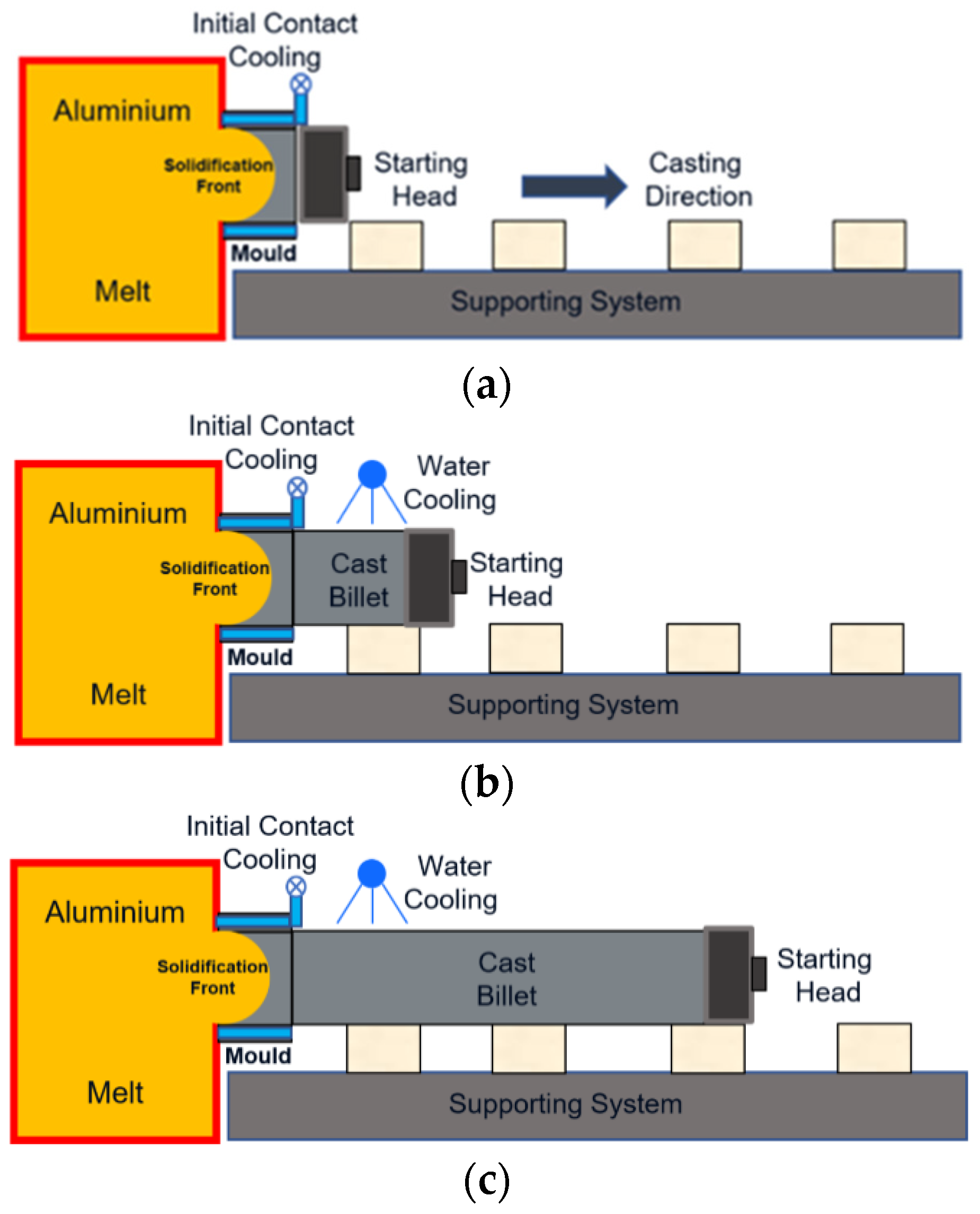
2. Dynamic Processes

The optimization of different industrial processes including, casting, extrusion, forging, and rolling have long been considered, and many technical\economic advantages on the one hand and also difficult technical challenges, on the other hand, have been examined. The use of numerical simulations for optimizing these processes has undoubtedly gained popularity in the last couple of decades and new and innovative methods have been developed to be a part of design-optimize-verify processes or even used as a part of real-time monitoring and automation in the production lines [7,8,9,10,11]. The FE and CFD solvers have traditionally been utilized for these material process simulations where multi-physical\phase and multi-scale aspects of the material evolutions have been considered.

The conventional meshing and spatial discretization schemes have initially been utilized in these numerical techniques to define a fixed number of simpler subspaces\elements with approximate or exact functions (e.g., shape functions). These discretized numerical domains are then formulated into an algebraic system of equations which can be solved with the FE and CFD solvers. However, many material processes, like casting, extrusion or even Additive Manufacturing (AM) processes are characterized by their gradual production in the time domain. These continuously growing domains for the dynamic processes are principally described with the rate of material and thermal energy insertion during the process (e.g., casting speed, AM deposition rate). The main challenges for the simulation of these processes are the dynamic nature of these numerical domains, their continuous material insertion, and the evolution of thermal energy characteristics during these processes.

Although today’s meshing technologies have become very efficient during simulations (e.g., adaptive re-meshing), even for the complex geometries and also bodies with large deformations, the issues of dynamic changes of the domain during simulations and their evolving discretization scheme have not been systematically addressed. For the dynamic processes like the casting process and AM, the traditional numerical discretization strategy was based on the domain discretization for the whole final part\billet. The generated elements in these domains are then deactivated at the start of the transient simulation to be later activated piece-wise based on the casting speed (or deposition rate) during the process simulation.

Although this “Block deactivation\activation Technique” (BT) can successfully be applied to some industrial casting applications like vertical and horizontal casting processes (shown in Figure 1), the size of the numerical matrices and system of equations is large for the duration of the transient analysis (deactivation of elements at the start of the process would not remove their matrices from the equation solver). To mitigate this problem, there have been some attempts to introduce innovative discretization techniques [12,13,14] for dynamic systems including mixed and merge/splitting element and cell division techniques. In these techniques, the numerical domain can be divided into Lagrangian, Eulerian, and Arbitrary Lagrangian-Eulerian (ALE) zones. For the casting and extrusion (and also AM) applications, the transient extension of the part during the simulation can numerically be modeled using the splitting element layers at interfaces. Although the approach can alleviate the existence of a large system of equations from the start of the simulation, it has limitations in terms of interface geometries and boundaries for the more complex dynamical systems.

For the process simulation of the continuous and semi-continuous casting and its complicated fluid-mushy-solid coupled analyses (e.g., multi-phase analyses), it is essential to use an advanced numerical approach, capable of dealing with melt flow, thermal energy transfer, solidification, and also solid-state conditions. The melt fluid flows into the mould and its low turbulence/laminar characteristics, mushy and solidification zone (with its metallurgical aspects), and also the final solid zones need to be simulated accurately to achieve desired results. These sophisticated numerical simulations have already found their way into the mainstream industrial tools [15,16,17] to enable the simulation of chain processes for production lines. Although the early multi-phase simulations of these processes are an important part of the framework, the details of these simulations are not discussed here in this paper. To limit the in-depth technical discussions within a single manuscript, only the thermal-mechanical simulations of dynamic material processes are presented herein. More technical discussions about the conventional material processes can be found in [18,19,20].

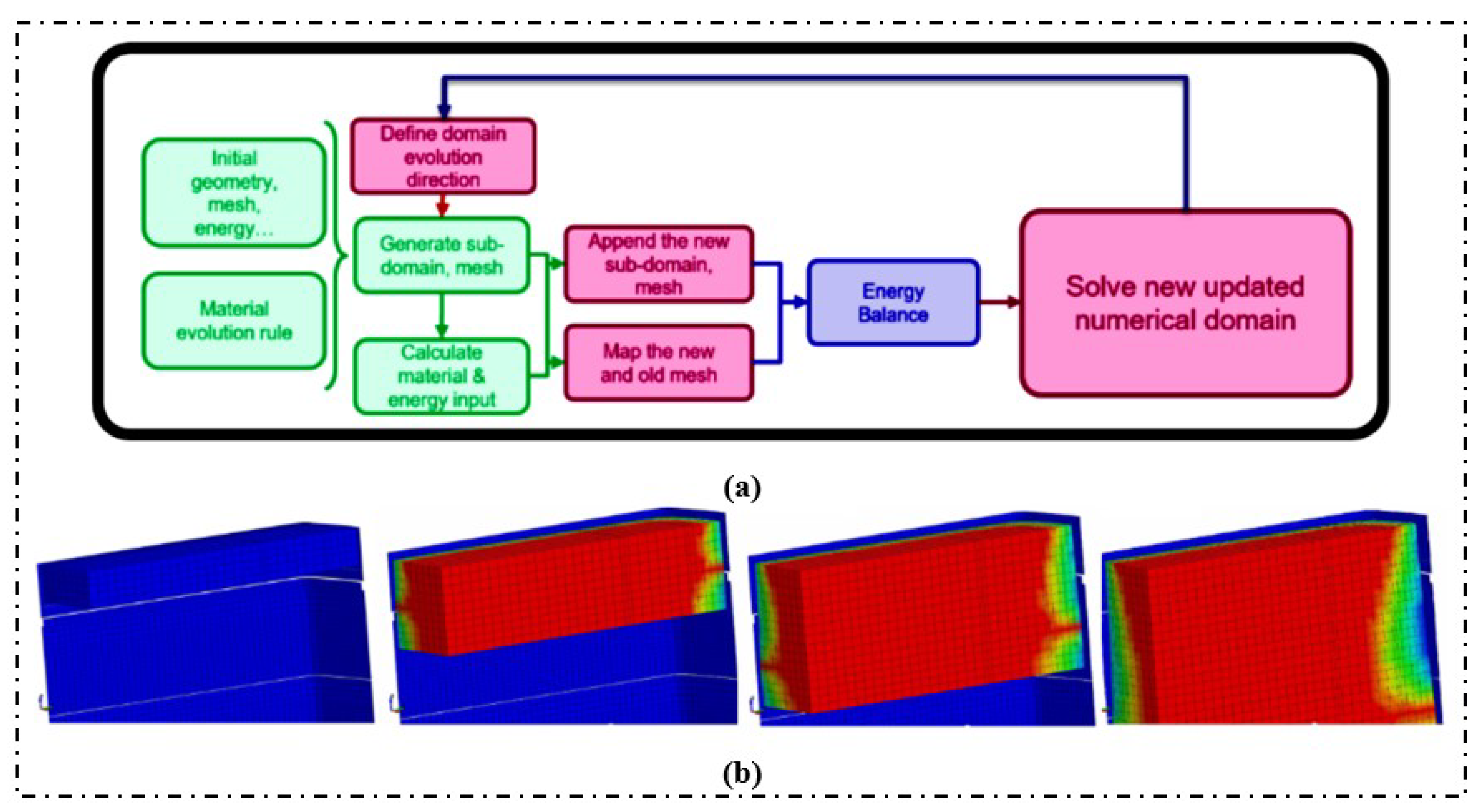
3. Evolving Domain Technique

The increasing computational power during the last couple of decades has greatly affected the way the traditional material process simulations were conducted and more advanced schemes like coupled multi-physical and multi-phase material modeling have quickly emerged. Furthermore, the pace of design for more energy-efficient and quality-oriented industrial processes has significantly picked up in the last two decades where more innovative and smart virtual tools are utilized to accelerate these processes.

The new concept of evolving domain and its Dynamic Mesh Technique (DMT) has been developed recently [20,21,22,23] to overcome numerical problems related to the continuous evolution and transient generation of numerical domains. It treats the extended parts of the domain as a dynamic zone (e.g., mesh block) which can be appended\evolved in a predefined or calculated manner and ultimately be attached to the main domain through a mapping-boundary concept. As the newly generated meshes are attached to the original domain, a mapping procedure would be performed to handle the new material\energy input.

For the mapping at the interfaces between the existing discretized domain with a newly appended mesh block and to overlap grids with multi-resolution (e.g., overlapping meshes with different sizes) some mathematical representations have already been developed. The Partition of Unity Finite Element Method (PUFEM), Overlapping Sphere Elements (OSE) and a few other techniques have already been proposed to handle the grid-inconsistency [24,25,26]. For overlapping meshes at the boundary of a numerical domain, let us assume two interfacing grids with overlapping conditions at the boundaries of Ω1 and Ω2 numerical domains. For linear finite element grids with base functions ${\{v_i\}}_{i\in I}$ and ${\{w_j\}}_{j\in J}$, the overlapping set can be written as [24,25,26];

$${\{{\varnothing }_1{v}_i,{\varnothing }_2{w}_j\}}_{i\in I,j\in J}$$

(1)

If the overlapping meshes are represented with a linear independent relation as;

$${\varnothing }_1{{\displaystyle \sum }}_i{\alpha }_i{v}_i+{\varnothing }_2{{\displaystyle \sum }}_j{\beta }_j{w}_j=0$$

(2)

and if it is assumed that ${\varnothing }_2=\mathrm{1}-{\varnothing }_1$ then it can be shown that;

$${\varnothing }_1\left({{\displaystyle \sum }}_i{\alpha }_i{v}_i-{{\displaystyle \sum }}_j{\beta }_j{w}_j\right)=-{{\displaystyle \sum }}_j{\beta }_j{w}_j$$

(3)

$${{\displaystyle \sum }}_i{\alpha }_i{v}_i-{{\displaystyle \sum }}_j{\beta }_j{w}_j=Const.$$

(4)

To form a stiffness matrix for the interfacing\overlapping meshes, an assembly can firstly be formed for non-overlapping elements (as a conventional assembly process) and secondly, overlapping elements’ terms can be entered with multiple entries. More comprehensive discussions about the multi-resolution interfacing\overlapping grids can be found in the literature [25,26].

Figure 2 shows a schematic workflow and dynamic mesh generation for the evolving domain framework where mesh blocks are inserted during the transient simulation at subsequent time steps. For the continuous casting and extrusion simulations, a directional vector (horizontal or vertical) can be predefined to start the directional boundary insertion and mapping scheme for the generated mesh blocks\layers to resemble the transient extension of the billet\part. The dynamically generated mesh blocks or element rows can be appended to the original numerical domain between restarts depending on the speed and requirement of the numerical model for the industrial process. As the numerical solution is performed on a full parallel-processing machine, decomposition of the extending domain for multiple instances of the solver at each restart shall independently be carried out for the transient solution. The generated element blocks (with the same or different sizes) are integrated into the original domain matrices by a reassembly process at restarts points (and become a part of the main domain) as the billet extension step with pre-defined casting speed comes to the end.

Additionally, for the estimation of the thermal energy evolution and cooling during the transient process, HTC calculations were carried out to calculate the cooling rates and thermal gradients. For continuous and semi-continuous casting processes, one of the popular cooling strategies is to use water spray cooling. The numerical modelings of cooling processes are also essential to develop a deep understanding of the thermal evolution and the volatile temperature fields during casting processes. In many casting processes, the cast billet is impinged by a water jet to extract the thermal energy from inside of the billet. During the cooling process, the billet undergoes large temperature fluctuations, especially near its surface. Hence, it is essential to investigate and control the thermal event to minimize the occurrence of defects on the surface or sub-surface (hot tearing, cold cracking…).

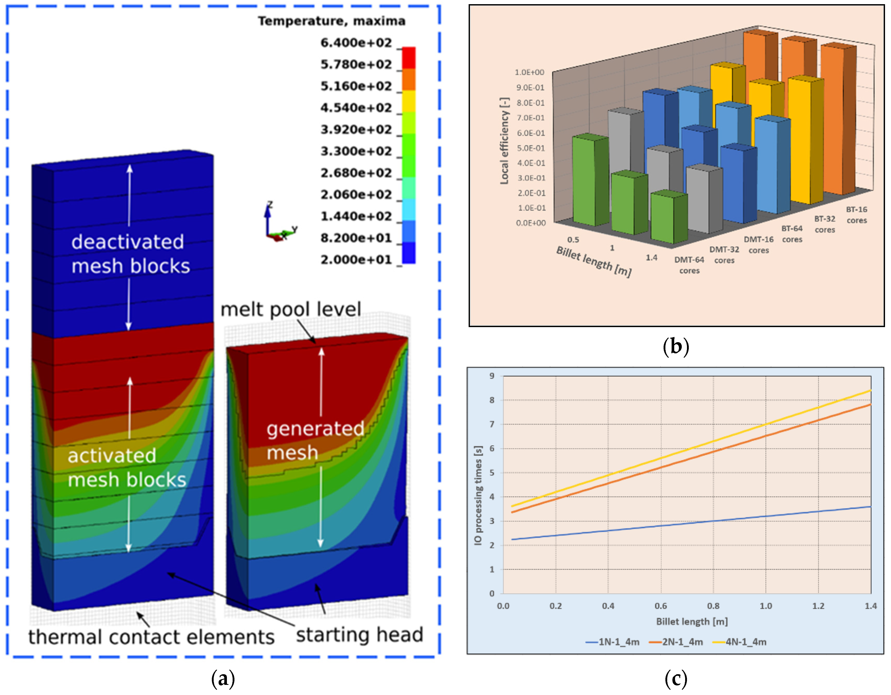
4. Computational Performance

For the continuous casting application, the issues of long billet sizes and time-dependent generation scheme based on a pre-defined casting speed are encouraging a new approach for simulating such processes. One of the main burdens of these new techniques is the computational time and resources. For dynamic systems, it is essential to have a strategy to evolve the numerical domain according to the real pace of the manufacturing process which ultimately delivers a dynamic and growing computational domain. The proposed DMT technique can deliver a method where accurate results can be obtained using growing and evolving domains [4,9,11]. The computational resources for this technique are commissioned gradually as the size of the real billet and its simulated counterpart are growing during the process. Restarting solvers at discrete time steps comes at additional costs for the repeated matrices’ assemblies and extra Input\Output (IO) activities.

The practical applications of the proposed DMT for real industrial cases can only be feasible when it can be shown that the technique is capable of competing with the best available techniques (e.g., BT) in terms of computational performance. To assess the computational efficiency of the DMT technique against the conventional BT a comprehensive numerical investigation has been carried out to study an industrial size vertical semi-continuous casting process. For the BT simulation, element blocks are predefined and the whole model is pre-loaded at the start of the simulation while the contacts between the blocks are activated consecutively.

Table 1. Defined parameters for casting process.

Melt Temperature [°C]	Billet Width [m]	Billet Thickness [m]	Casting Speed [m s−1]	Cooling Water Temperature [°C]	HTC- Air Cooling [kW m−2 K−1]	HTC- Water Cooling [kW m−2 K−1]
630	1.24	0.3	0.01	20	1.5 (average)	11 (average)

shows the casting process parameters for both simulation techniques, while

Table 2. Scenarios Table for DMT and BT case studies using a single computing node with 16 cores.

Scenario No.	Billet Length [m]	No. of Elements	CPU Time DMT [s]	CPU Time BT [s]	IO Time DMT [s]	IO Time BT [s]	CPU Ratio DMT/BT
S1	0.5	27,189	16,345	20,581	78.62	6.90	79%
S2	1	41,357	45,577	77,387	179.18	7.02	59%
S3	1.4	59,573	84,545	163,063	271.84	13.77	52%

shows a scenario table designed to assess the computational time and resources of both techniques for all scenarios on a single computing node. Additionally, Figure 3a shows the BT and DMT numerical models for the vertical semi-continuous casting process and their meshing strategies. Due to the double symmetric condition of the rectangular billet, only a quarter of the billet is modeled and meshed for the transient simulation to save computational time and resources. As it is shown in Figure 3a, different meshing and contact strategies were used to carry out the casting simulations for DMT and BT. While both techniques have employed contact elements to simulate the cooling boundaries (air and water cooling), for BT, the contacts had to be set up for the full length of the billet. Alternatively, for DMT, as new mesh layers are generated and attached to the main domain at solver restarts, contact setups needed to be updated [4,9,11].

The computational efficiency of DMT in terms of CPU time and IO resources should be investigated using industrial-scale case studies on a parallel computing platform. Hence, a table for numerical simulations of industrial-scale scenarios has been prepared for estimation of computational efficiency. Table 2 shows the simulated scenarios for both DMT and BT models on different numbers of computing nodes. For the purpose of comparison, numerical models with three different geometries (for the billet lengths 0.5 m, 1 m, and 1.4 m) were created and their corresponding structured meshes were generated accordingly. These models were simulated on a parallel computing platform with the technical specifications shown in

Table 3. Technical specifications and version of operating software for parallel computing nodes.

CPU Name	No. of Sockets	Cores per Socket	Total Memory [MB]	Communication Between Nodes	Parallelization Scheme	LS-DYNA Release	Accuracy
Intel Xeon E5-2687W v4	2	8	65536	InfiniBand	Platform MPI 08.02.00.00 [10060]	MPP R8.1.0	Double precision

.

To compare the simulation results, the computational time-history results were post-processed to calculate the CPU and IO computational times. The three-dimensional plot of local computational efficiency against three billet lengths and the number of computational cores is shown in Figure 3b. The local efficiency can be defined as the ratio of the total simulation time of a base scenario for the specified billet length (i.e., wall clock time) divided by the CPU time for each scenario. The most efficient scenario using 16 cores for the DMT technique was used as a base scenario for each billet length. Accordingly, the higher the efficiency values shown in Figure 3, the lower the total simulation times for the casting scenarios.

The results of the comparative study presented in Figure 3 show that concerning numerical efficiency, DMT can outperform BT almost in every scenario. It can also be clearly seen how the billet length and the parallelization influence the computational efficiency where DMT can benefit more from heavy parallelization than BT. Only in the case of 64 cores and only for the short billet length of 0.5 m, BT can slightly beat DMT using 16 cores [4]. Furthermore, Figure 3c shows the increase in IO processing times for DMT at each restart point (for 1.4 m length billet) using different numbers of computational nodes (1, 2, and 4 number of nodes). Due to the increased number of elements and thus history variables, the time and effort for reading and writing data, decomposing the mesh for parallelization, and initializing the matrices increase steadily over the whole transient simulation. It is also clear that using more than one computational node leads to a significant increase in input/output time while the difference between using 2 nodes (16 cores) and 4 nodes (64 cores), on the other hand, is not significant. Despite the higher IO time for the DMT, the total simulation wall clock time is still significantly lower than the conventional technique due to the fact that the CPU computational time is generally more than two orders of magnitude larger than IO times for real-size casting applications.

5. Conventional Cooling Models

Different aspects of numerical simulations of material processes are founded on complicated phenomena governed by the multi-physical and multi-phase interactions including thermal evolution and heating\cooling modeling. The cooling modelings during these material processes and their numerical simulations are traditionally based on a methodology of using theoretical and analytical knowledge along with some practical experiences. As conventional water impingement cooling is still popular in many material processes, the numerical modelings of these processes are essential to developing a deep understanding of thermal evolutions and their effect on final product quality.

During these processes (e.g., casting, rolling, extrusion, etc.), billet\parts are impinged with a water jet to extract thermal energy and to cool down to room temperature. Although a lot of research has been conducted in the last twenty years to numerically calculate\estimate the thermal evolution and heat transfer phenomena during industrial material processes, the complex multi-physical\phase nature of these events could not fully be described. Hence, simpler analytical estimations of Heat Transfer Coefficient (HTC) during these processes have broadly been used to accelerate the modeling process. The mathematical representation of the cooling process on hot surfaces can be expressed with the simplified governing equations for the water spray cooling system as [27,28,29];

$$\nabla .U=0\hspace{1em}\hspace{1em}\frac{\partial U}{\partial t}=-\nabla \left(\frac{P}{\rho }\right)+\frac{1}{Re}{\nabla }^{2}U$$

(5)

where U, P, ρ and Re are velocity vector, pressure, density, and Reynolds number, respectively. The spray wet area can also be defined as;

$$A=f\left(x,y,z\right)\frac{Q}{V_s}$$

(6)

where f(x,y,z), vs. and Q are coordinate distribution function, surface flow rate, and water flow rate, respectively. Various parameters would affect the thermal energy dissipation during water spray cooling, namely: temperature difference between billet surface and water, water flow rate, angle of impingement, water quality, surface roughness, and some other minor parameters. Since, the type of boiling regime on the hot surface has major effects on the heat dissipation rate, the complex interaction between surface/steam/water and air would determine the real cooling HTC. Figure 4 shows a schematic bubble generation and departure on a horizontal hot surface during a water spray action.

Although there have been many attempts in recent years to carry out interfacial HTC estimations based on the inverse heat transfer calculations using available experimental data (with fitting techniques), the generality and accuracy of these estimation techniques have not been verified [30,31]. To make the HTC estimations simpler, the thermal energy transfer during cooling can be assumed as the summation of different interchanging mechanisms between a hot surface and the water as;

$$q_T=q_1+q_2+q_3$$

(7)

where q₁, q₂ and q₃ are single-phase convective, evaporation, and quenching heat flux densities, respectively. With some mathematical manipulation, for the case of continuous liquid phase (water) and dispersive gases (water vapor and air), the three-phase continuity equation for phase k can be written as [32,33]:

$$\frac{\partial {\alpha }_k}{\partial t}+\nabla ({\alpha }_k{\overrightarrow{U}}_k)=\frac{{\Gamma }_{ki}-{\Gamma }_{ik}}{{\rho }_k}$$

(8)

where k denotes the phase and can be either liquid or gas and i is the non-k phase. The α, ρ, and U represent the phase volume fraction, density, and velocity vector respectively. More detailed discussions about the conventional spray-cooling modeling can be found in [27,28,29,30,31,32,33].

6. Hybrid Cooling Models

The use of hybrid physical-data-driven modeling and its application in material science and engineering have increasingly been promoted over recent years and the implementation of ML and AI technologies within alloy designs and processes have gradually been utilized. These emerging techniques have a great potential for the future of material process engineering and industrial manufacturing where it has already been proven that their potential to generate values in various material process applications and material modeling domains are significant [34,35]. For the material process simulations, ML and AI mean algorithm-based and data-driven schemes which enable better representations of phenomena with more accurate predictions and better continuous learning and improvement. The hybrid models are categorically grouped into different classes, namely; auxiliary, augmented, full, and dynamic hybrid models where different applications can be handled using an appropriate type of hybrid model. The description of these models can briefly be presented as;

➢

For auxiliary hybrid models, parameters in the physical/empirical models are function-fitted using ML and AI tools

➢

In augmented hybrid models, physical models are augmented with terms derived by function-fitting features of ML and AI tools

➢

Fully hybrid models where data trends from ML and AI are used along with physical laws to derive the hybrid model.

➢

Trained (or dynamic) hybrid models where the existing hybrid model is a subject of ML and AI tools for improvement

As these techniques are becoming ostensible for many materials and process modeling applications including dynamic casting and forming applications, the need for a greater understanding of technology utilization has raised within material and process simulation communities. The modeling capabilities of these techniques share the same fundamental intentions, namely; faster and more accurate modeling and the ability to dynamically change the rules and functions using new emerging data.

To ease the analytical overburden for the cooling modeling, the concepts of augmented hybrid modeling have willingly been employed here to estimate HTCs during the casting process. Since the mass conservation of the sum of the volume fractions in (8) should be unity (${\sum }_k{\alpha }_k=1$), the momentum terms for any of the phases in the equation should be conserved as [36,37,38,39,40];

$$\frac{\partial }{\partial t}\left({\alpha }_k{\rho }_k{U}_k\right)+\nabla .\left({\alpha }_k{\rho }_k{U}_k{U}_k\right)=-{\alpha }_k\nabla p+{\alpha }_k{\rho }_{k}g+\nabla .{\alpha }_k\left({\tau }_k+{\tau }_k^t\right)+M_k$$

(9)

where p and g are pressure and gravitational acceleration. The M_k is the total interfacial force which can be defined as the rate of bubble generations and their movement relative to the hot surface during material processes as [36,37,38,39,40];

$$M_k=F_D+F_W+F_L+F_B+F_V+F_{TD}+{\sum }_{j=1}^N\left({\dot{m}}_{jk}{U}_j-{\dot{m}}_{kj}{U}_k\right)$$

(10)

where F_D, F_W, F_L, F_B, F_V and F_TD are the drag, the wall lubrication (smoothness), lift, buoyancy, virtual mass, and turbulence drag forces (the Basset force is ignored herein due to negligible effects). The last term on the right-hand side of the equation is defined as momentum transfer associated with mass transfer. The energy conservation equation for each phase can also be written as [36,37,38,39,40];

$$\frac{\partial }{\partial t}\left({\alpha }_k{\rho }_k{h}_k\right)+\nabla .\left({\alpha }_k{\rho }_k{U}_k{h}_k\right)-\nabla .\left[{\alpha }_k\left({\lambda }_k\nabla T_k+\frac{{\mu }_t}{{\sigma }_h}\nabla h_k\right)\right]=Q_k$$

(11)

where h, λ, T and Q are enthalpy, thermal conductivity, temperature, and interfacial heat transfer respectively. For the wall lubrication force (also known as Frank force), which is the effect that moving the bubbles away from the hot surface, the values can be estimated as [36,37,38,39,40];

$$\begin{gathered} F_w={\alpha }_d{\rho }_c{C}_w{\left\{\left(v_d-v_c\right)-\left[\left(v_d-v_c\right).n_w\right]n_w\right\}}^2{n}_w{C}_W= \\ {C}_{WE}max\left[0,\frac{1}{C_{WD}}\frac{1-\frac{y_w}{C_{WC}{d}_b}}{y_W{\left(\frac{y_W}{C_{WC}{d}_b}\right)}^{p-1}}\right] \end{gathered}$$

(12)

where n_w, C_w, C_wE are the normal unit vector for the hot surface, the wall lubrication coefficient, and bubble Bond coefficient. The p, C_WC, and C_WD are correction coefficients and can be assumed as p = 1.7, C_WC = 10 and C_WD = 6.8 for the casting cooling spray system. The bubble Bond coefficient can also be estimated as,

$$C_{WE}=\{\begin{array}{c}{e}^{-0.933E+0.179}\hspace{1em}1\le E\le 5\\ 0.007E+0.04\hspace{1em}5\le E\le 33\hspace{1em}E=\frac{\Delta \rho g{L}^2}{\sigma }\\ 0.179\hspace{1em}33<E\end{array}$$

(13)

where E is the bond number which is defined as a dimensionless number measuring the importance of surface tension forces compared to body forces and is used to characterize the shape of bubbles moving in a continuous fluid. The Δρ, L and σ are density differences, characteristic length, and surface tension force per unit length. For the spray cooling during the casting process, the bond number can be written as [36,37,38,39,40];

$$E=\frac{g\left({\rho }_c-{\rho }_d\right)d_b}{\sigma }$$

(14)

where d_b is the expected bubble diameter. Although the drag force F_D can approximately also be estimated using analytical calculations (with some simplified assumptions), the low accuracy of the results would hamper the HTC calculations for jet and spray cooling. Hence, an augmented hybrid model is used here to combine the analytical and data-driven techniques for the calculation of the interfacial force.

To start generating data for the calculation of the bubble drag force, a series of numerical simulations using detailed CFD modelings have been performed. A scenario table has then been defined for the drag force calculations based on varying bubble diameters and flow velocities.

Table 4. Numerical simulation scenarios for different bubble diameters and water flow rates.

	Vel. [m/s]	0.1	0.2	0.5	0.8	1	1.5	2	2.5	3	4
Dia. [m]
0.001		×	×	×	×	×	×	×	×	×	×
0.002		×	×	×	×	×	×	×	×	×	×
0.005		×	×	×	×	×	×	×	×	×	×
0.02		×	×	×	×	×	×	×	×	×	×
0.05		×	×	×	×	×	×	×	×	×	×
0.1		×	×	×	×	×	×	×	×	×	×

shows the scenario table for the numerical simulations where different scenarios based on bubble diameters and water flow rate (e.g., water velocity at nozzles) are defined. For the data handling and postprocessing of the drag force data, the GASR technique has been employed. GASR is one of the interesting data processing techniques where measured and/or calculated data can be fitted by suitable mathematical formulae (from a different family of functions) using genetic and\or evolutionary algorithms. The technique has gradually been developed for computer implementation in recent years and some computer tools are already available based on GASR technologies. HeuristicLab [6] is one of the open-source academic software tools which have been developed to deal with a variety of data-driven modeling problems. It is prominently useful for problems where computational simulations are combined with optimization and design features within science and engineering research activities.

The verification of drag force calculation for a single bubble has initially been carried out using simplified analytical and 2D detailed CFD techniques. One of the simple and popular analytical technique which can be used to approximate the bubble drag force can be written as [36,37,38,39,40];

$$F_D=C_D\frac{1}{8}{\rho }_c{A}_{int}\left|v_r\right|v_r{}^{\alpha }$$

(15)

$$C_D=\frac{24}{R{e}_b}\left(1+0.15R{e}_b{}^{0.678}\right)R{e}_b=\frac{{\rho }_c\left|v_r\right|d}{{\mu }_c}$$

(16)

where C_D, ρ_c, $A_{int}=\frac{\pi d^2}{4}$, d, α, and v_r are the drag coefficient, density of continuous phase (water), interfacial area, bubble diameter, correction factor, and the phase’s relative velocity (v_r = v_d − v_c, the velocity difference between continuous and disperse phases), respectively. Figure 5 shows the comparison of drag forces for a single bubble using the simplified analytical (red) and the detailed CFD techniques (blue), assuming d = 2 mm, α = 1.5, and ρ_c = 1000 kg/m³.

The drag force data for the GASR multi-dimension regression analyses have then been generated using the results of the detailed CFD simulations. For the initial velocity field near the hot surface, global transient CFD analyses have been performed to calculate the water velocity field near the wall where bubbles are generated. Figure 6a,b show the global CFD simulation for the water cooling impingement on the billet surface and the thermal boundary setup for the vertical casting process. While Figure 6c show the detailed CFD simulations for the bubble dynamics for two different bubble diameters.

The calculation of bubble’s drag forces using detailed CFD simulations has broadly been carried out for all planned scenarios and a small database has been generated for GASR training. In the work herein, the method of symbolic regression is freely used to obtain mathematical expressions of functions that can fit the cooling data based on simple rules and broad generalization. It differs from the conventional regression analyses (linear or nonlinear) where parameters are optimized in the mathematical model, rather it generates a routine to create models and their parameters for better a fitting scheme or for the purpose of getting better insights into the dataset.

Figure 7 shows the graphical presentation of the tree diagram for GASR function fitting along with resulting expressions for the bubble drag force with varying water velocities and the bubble diameters. The calculation of HTC values on the interface between the hot billet surface and water is generally governed by the classical thermal energy transfer law;

$$q=HTC\left(T_b-T_w\right)$$

(17)

where T_b, T_w are temperatures of billet surface and impinging water. As the water flow momentum\velocity and pressure vary over the billet surface during the cooling process, the HTC is not uniform over the whole billet surface. Additionally, the HTC calculations for the casting processes can be split into four distinct temperature ranges (see

Table 5. New hybrid HTCs’ equations for water impingement.

Zone Number	HTC Estimations
I–pre-boiling zone 40 < Tb < 100 °C	$HT{C}_{pre}=\alpha {\left(\frac{Q}{L_b}\right)}^{\beta }\left(7e2\ast T_b-1.67e3\right)$
II–nucleate boiling zone 100 < Tb < 235	$HT{C}_{nu}=\left(\frac{\mu H_{fg}}{T_{sat}{c}_f^{\alpha }}\right){\left(\frac{C_p{T}_b}{H_{fg}}\right)}^{\alpha }{\left(\frac{\sigma \mu C_p}{Kg({\rho }_w-{\rho }_v{}_{})}\right)}^{\beta }$
III–transition boiling zone 235 < Tb < 400	$HT{C}_{tra}=HT{C}_{nu}\left(1-{\left(\frac{T_b-T_{CHF}}{T_b}\right)}^{\gamma }\right)$
IV–film boiling zone 400 < Tb < 550	$HT{C}_f=HT{C}_{tra}\left(1-{\left(\frac{T_b-T_{Le}}{T_b}\right)}^{}{(H_1+H_2)}^{\lambda }\right)$ $H_1=\frac{\gamma }{T_b}\times {\left(\frac{k_w^{3}g{\rho }_w{H}_{fg}\left({\rho }_w-{\rho }_v\right)\left(1+\frac{c_p{T}_b}{2H_{fg}}\right)}{{\mu }_w{T}_b{\left(\frac{\sigma }{g\left({\rho }_w-{\rho }_v\right)}\right)}^{\beta }}\right)}^{\alpha }$ $H_2=\frac{5.4\times {10}^4}{T_b}\left(1+0.055T_b\right)v_s^{\kappa }$

), namely;

➢

Pre-boiling: surface temperature below the water boiling temperature (T < 100°C) where single-phase calculation can be used to estimate the HTC values

➢

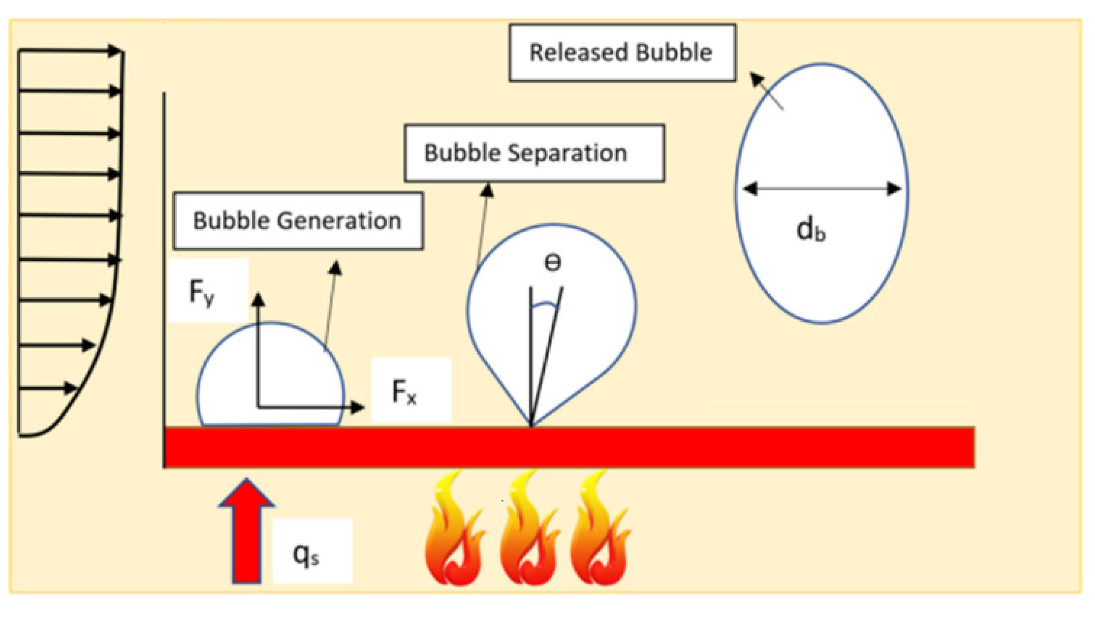
Nucleate boiling: surface temperature between water boiling temperature and Critical Heat Flux (CHF) temperature where nucleate the boiling regime is dominant. The formation of the discrete bubbles and their movement under drag, lift, and Frank lubrication forces (as discussed earlier) enhances the local fluid motion resulting in an increasing convective HTC. At higher billet surface temperatures near the CHF temperature, the discrete bubbles would coalesce into large size bubbles which further enhances the water flow (the so-called “fully developed nucleate boiling regime”). The rate of change for the surface HTC in the nucleate boiling regime is significant even with small surface temperature changes. For many industrial casting applications, the water-sprayed nucleate boiling regime is preferred since it is generating a high cooling rate.

➢

Transition boiling: surface temperature between CHF and Leidenfrost temperatures where transition boiling regime is taking place. The transition boiling regime and its modeling is one of the challenging issues for HTC calculations during industrial processes. In this type of boiling regime, the surface thermal energy exchange reduces as the billet surface temperature increases.

➢

Film boiling: surface temperature above the Leidenfrost temperature where vapor films are covering the surface of the hot billet. The modeling of cooling for this temperature range can be divided into several cooling regimes based on the different interface of fluid (water) and vapor as continuous, discrete, stable, and unstable.

The continuous HTC functions for the variation of billet surface temperatures have to be defined from hotter temperatures at the top of the billet to the cooler temperatures at the lower elevations to enable the simulation of the whole casting process at an industrial scale.

7. Hybrid-Evolving Technique: Case Study

To investigate the application of the evolving domain technique combined with the hybrid cooling models for industrial casting processes, a conventional vertical casting process has been simulated. As stated earlier, the conventional approach for dynamic systems like casting processes on FE solvers is to pre-mesh the whole cast domain (since the final shape of the domain is known) and to activate elements during the simulation. The CPU computational time and memory storage issues are the main drawbacks of such an approach which restricted the application of the technique for practical industrial casting simulations (especially for limited in-core computer storage space). Hence, for the continuous casting applications herein, a gradual extension of the numerical domain during the solution could avoid solving large matrices for all time steps and save computer resources during the calculation.

As part of the multi-physical and multi-phase simulation framework, the hybrid-evolving technique deals with the cooling phenomena at boundaries while the dynamic mesh module with its efficient parallel-processing scheme can perform fast and accurate FE analyses. For the casting process case study herein, the combination of hybrid physical-data driven technique and the dynamic generative computational scheme has been employed to promote the application of these new trends in the material science

7.1. HTC Estimations

For the vertical casting application, the thermal energy transfer during the process is complicated and cumbersome to accurately predict for the final FE simulations. The casting HTC values change rapidly during the startup condition where different cooling regimes add to the modeling complications. The HTCs generally rise rapidly with the increasing billet surface temperatures until a critical temperature is reached where the unstable and film boiling regimes would reduce the associated HTCs. As stated earlier, the estimation of CHF temperature point and its associated heat flux can help to understand and optimize the billet surface cooling rates and thermal-mechanical stress\strain conditions within the cast billet. The critical billet surface temperature for this study can be estimated at 220 °C to 275 °C (depending on surface roughness and water quality) where cooling on the hot billet surface is achieved by heat transfer from the billet to a free-falling film of water running down on the outside of the billet surface.

Using the analytical and hybrid physical-data-driven models presented in the previous section, a new set of HTC equations has been derived to model the heat energy evolution during the casting process. Appendix A and Appendix B present a brief description of the basic mathematical concepts and their parameter definitions while Table 5 and Figure 8 show the final derived HTC equations and their graphical representations. Although the use of a hybrid modeling technique results in long equations for the HTC estimations, the computer implementations of these equations would ease the calculation times.

As it can be seen in Figure 8, the HTC values are rising towards the CHF point where maximum cooling can be achieved for both experimental measurements and the hybrid model. Although the maximum thermal heat transfer for both models is similar the HTC measured and calculated values below CHF shows some inconsistency. At first glance, it seems that the hybrid model is overestimating the HTC values for billet surface temperatures between 60 °C to 230 °C. The experimental HTC graph is calculated based on the method in [41,42,43] where temperature measurements were obtained using a set of installed thermo-couples. Figure 9 shows the in-house testing apparatus for plate cooling tests along with the thermo-couple arrangements and the view of the water jet impingement. Using the apparatus, water can be impinged on a fixed and stationary plate using an appropriate size nozzle. Due to difficulties of measurements on the surface of the hot plate, the thermo-couples were mounted on the back of the plate inside a set of pre-drilled holes. The distance of these thermo-couples to the surface of the plate is a minimum 3 mm which makes the recorded temperatures within the bulk of the plate (not exactly on the surface). Hence, for these thermo-couples, the large thermal gradient forming at the very near of the plate surface cannot be captured accurately. Subsequently, the final HTC estimations using the experimental data seem to show underestimated values (e.g., showing zero HTC at about 60 °C) which may explain some of the inconsistencies between the recorded and calculated values at the lower temperatures.

7.2. Hybrid Evolving Simulation

In this case study, an industrial contact-less vertical casting process with rectangular cross-section has been modeled using the dynamic and evolving domain technique [4]. To avoid the complicated mold-filling and fluid-thermal-mechanical interaction simulations, a simple filling condition has been estimated and an initial state of the billet is assumed (e.g., after 50 mm of casting) along with initial thermal conditions. A preliminary structured mesh has been generated with thermal and displacement degrees of freedom. The convection and radiation of the melt (at the top of the mold) are taken into account using the results of free-convention CFD simulations (shown in Appendix B, Figure A1).

For the water-cooling HTCs, the values based on the hybrid modeling have been implemented and used for the rectangular quarter-model billet (using input parameters shown in Appendix B,

Table A1. Definition of parameters for hybrid HTCs equations.

Zone Number	Parameters	Validity
I–pre-boiling zone	Q–water flow rate [m3/sec] Lb–billet perimeter [m] Tb –billet surface temp. [°C] α = 1.35 β = 0.3	40 < Tb < 100
II–nucleate boiling zone	μ = 0.000267 [Ns/m2] Hfg = 2257e3 [J/kg] cf = 0.016 [J/s] Cp = 4219 [J/kg K] K = 0.68 [W/m K] g = 9.81 [m/s2] rw = 995 [kg/m3] rv = 0.6 [kg/m3] σ = 0.059 [N/m] α = 0.8 β = −0.515	100 < Tb < 235
III–transition boiling zone	TCHF = 235 [°C] g = 0.42	235 < Tb < 400
IV–film boiling zone	vs= 1 [m/s] α = 0.4 β = 0.5 $\gamma$ = 0.5 k = 0.6 l = 0.15	400 < Tb < 550

). Figure 10 shows the FE simulation of the billet and the resulting cooling curves for the Hybrid-evolving model. Figure 10a,b show the generation of dynamic mesh layers with their temperature contours during the evolving scheme for the billet quarter model, while Figure 10c shows the temperature comparison for the measured and simulated billet surface temperatures below the water impingement zone. As it appears from the comparison of the cooling curves, although the hybrid cooling model can predict the temperature gradient at the start of the casting process relatively well, it shows some degree of instability in the transition boiling zone (temperature between 280 °C to 400 °C). Despite all the efforts to adjust the data on the simulated HTCs (results using the hybrid cooling model) to the phenomena at this temperature range, due to the difficulties in the modeling of the stochastic unstable film formation on the billet surface (film formation and breakage) the results show some degrees of discrepancy.

8. Conclusions

The hybrid-evolving approach introduced in this paper employs a new numerical evolving-domain technique combined with analytical-numerical-data driven hybrid models to simulate industrial casting processes. One of the advantages of this combined approach is to increase the accuracy and flexibilities of the process simulations while limiting the required computational time and resources. The technique relishes enough agility and flexibility to be implemented on mainstream commercial solvers for material processes. The framework is also easily adaptable to various dynamic material processes and provides a practical simulation routine for these processes at an industrial scale.

At the start of the manuscript, some technical aspects of the new evolving domain and dynamic mesh technique have shortly been presented and the computational performance of the technique is investigated. In the following parts of the paper, the contagious concepts of multi-phase cooling modeling combined with its augmented genetic-algorithm ML model have briefly been scrutinized and the potential application of the method for industrial material processes are highlighted using a case study for the vertical casting application.

At the first glance, it can be presumed that for the evolving domain technique the mandatory repeated initializations and solver matrices’ re-assembly processes at every restart can introduce some disadvantages in terms of computational efficiency. However, detailed computational investigations have proved that processing smaller size matrices used throughout the simulations in this technique can outperform the conventional simulation techniques, especially on the parallel computational nodes. Furthermore, there is a possibility to shorten IO time for these initializations using embedded mesh data within the active computer memory of the FE solver. Thereby, the required input data could be passed to the solver directly instead of the conventional way via external input files.

As a final statement, the intention herein is to promote and encourage the use of a combination of hybrid modeling techniques with the latest developments on dynamic process simulations to upgrade computational material science to the next level. The opportunity to follow the trend on the new hybrid modeling schemes for further material processes would be taken and this would be the subject for the extension of the research work presented herein.

References

1. Horr, A.M. Multi-resolution simulations of material processes for e-mobility applications. In Proceedings of the 7th Transport Research Arena TRA 2018, Vienna, Austria, 16–19 April 2018. [Google Scholar] [CrossRef]
2. Farias A de de Almeida, S.L.R.; Delijaicov, S.; Seriacopi, V.; Bordinassi, E.C. Simple machine learning allied with data-driven methods for monitoring tool wear in machining processes. Int. J. Adv. Manuf. Technol. 2020, 109, 2491–2501. [Google Scholar] [CrossRef]
3. Tao, F.; Cheng, J.; Qi, Q.; Zhang, M.; Zhang, H.; Fangyuan, S. Digital twin-driven product design, manufacturing and service with big data. Int. J. Adv. Manuf. Technol. 2018, 94, 3563–3576. [Google Scholar] [CrossRef]
4. Horr, A.M.; Kronsteiner, J. On Numerical Simulation of Casting in New Foundries: Dynamic Process Simulations. Metals 2020, 10, 886. [Google Scholar] [CrossRef]
5. Horr, A.M. Notes on New Physical & Hybrid Modelling Trends for Material Process Simulations. J. Phys. Conf. Ser. 2020, 1603, 012008. [Google Scholar]
6. Wagner, S.; Affenzeller, M. HeuristicLab: A Generic and Extensible Optimization Environment. In Proceedings of the International Conference in Coimbra, Portugal, 18–19 July 2005; Adaptive and Natural Computing Algorithms; Springer: Berlin/Heidelberg, Germany, 2005; pp. 538–541. [Google Scholar]
7. Vijayaram, T.R.; Sulaiman, S.; Hamouda, A.M.S.; Ahmad, M.H.M. Numerical simulation of casting solidification in permanent metallic molds. J. Mat. Pro. Technol. 2006, 178, 29–33. [Google Scholar] [CrossRef]
8. Zhihong, G.; Hua, H.; Yuhong, Z.; Shuwei, Q. Numerical Simulation of Squeeze Casting of AZ91D Magnesium Alloy. In Proceedings of the 2010 International Conference on Digital Manufacturing & Automation, Changcha, China, 8–20 December 2010; pp. 30–33. [Google Scholar]
9. Brötz, S.; Horr, A.M. Framework for progressive adaption of FE mesh to simulate generative manufacturing processes. J. Manuf. Lett. 2020, 24, 52–55. [Google Scholar] [CrossRef]
10. Lindwall, A.L.J.; Lindgren, L.E. Thermal FE-simulation of PBF using adaptive meshing and time stepping. In Proceedings of the Simulation for Additive Manufacturing, Munich, Germany, 11–13 October 2017; pp. 62–63. [Google Scholar]
11. Horr, A.M. Computational Evolving Technique for Casting Process of Alloys. J. Math. Probl. Eng. 2019, 2019, 6164092. [Google Scholar] [CrossRef] [Green Version]
12. Claus, S.; Bigot, S.; Kerfriden, P. Cutfem Method for Stefan-Signorini Problems with Application in Pulsed Laser Ablation. SIAM J. Sci. 2018, 40, B1444–B1469. [Google Scholar] [CrossRef]
13. Bastian, P.; Engwer, C. An unfitted finite element method using discontinuous Galerkin. J. Num. Meth. Eng. 2009, 79, 1557–1576. [Google Scholar] [CrossRef]
14. Fausty, J.; Bozzolo, N.; Muñoz, D.; Bernacki, M. A novel level-set finite element formulation for grain growth with heterogeneous grain boundary energies. J. Mat. Des. 2018, 160, 578–590. [Google Scholar] [CrossRef]
15. Kleeberg, C. Latest Advancements in Modelling and Simulation for High Pressure Die Castings. In Proceedings of the ALUCAST, Chennai, India, 3–5 December 2010; Aluminium Casters’ Association. pp. 1–18. [Google Scholar]
16. Haldenwanger, H.G.; Stich, A. Casting simulation as an innovation in the motor vehicle development process. In Modeling of Casting, Welding and Advanced Solidification; Process IX, SIM 2000; Sahm, R., Hansen, P.N., Conley, J.G., Eds.; United Engineering Foundation: Philadelphia, PA, USA, 2000. [Google Scholar]
17. Malik, I.; Anwar Sani, A.; Medi, A. Study on using Casting Simulation Software for Design and Analysis of Riser Shapes in a Solidifying Casting Component. J. Phys. Conf. Ser. 2020, 1500, 012036. [Google Scholar] [CrossRef]
18. Francis, L. Materials Processing, A Unified Approach to Processing of Metals, Ceramics and Polymers; Academic Press: Cambridge, MA, USA, 2015; pp. 10–13. [Google Scholar]
19. Zhang, L.; Allanore, A.; Wang, C.; Yurko, J.A.; Crapps, J. Materials Processing Fundamentals; John Wiley: Hoboken, NJ, USA, 2013; pp. 63–72. [Google Scholar]
20. Horr, A.M. Integrated Material Process Simulation for Lightweight Metal Products. In Computational Methods and Experimental Measurements XVII; WIT Transactions on Modelling and Simulation; WIT Press: Southampton, UK, 2015; Volume 1, pp. 201–212. [Google Scholar]
21. Horr, A.M.; Kronsteiner, J.; Mühlstätter, C. Recent Advances in Aluminium Casting Simulation: Evolving Domains & Dynamic Meshing. In Proceedings of the Congress ALUMINUM, Verona, Italy, 20–24 June 2017; pp. 20–24. [Google Scholar]
22. Horr, A.M. Thermal Energy Approach for Aluminium Process Simulations: Source-Capacity Technique. J. Mater. Today Proc. 2019, 10, 263–270. [Google Scholar] [CrossRef]
23. Horr, A.M. On Analytical Concepts of Novel Multi-Resolution Casting Simulations. Proc. IOP Conf. Ser. Mater. Sci. Eng. 2019, 529, 012055. [Google Scholar] [CrossRef]
24. Liu, F.; Nashed, Z.; N’Guerekata, G.; Pokrajac, D.; Qiao, Z.; Shi, X.; Xia, X. Advances in Applied and Computational Mathematics; Nova Science Publishers: New York, NY, USA, 2006; pp. 38–46. [Google Scholar]
25. Cai, X.C.; Dryja, M.; Sarkis, M. Overlapping Nonmatching Grid Mortar Element Methods for Elliptic Problems. SIAM J. Num Anal. 1999, 36, 581–606. [Google Scholar] [CrossRef] [Green Version]
26. Mingyan, H.; Ziping, H.; Cheng, W.; Pengtao, S.; Shuang, Z. An overlapping domain decomposition method for a polymer exchange membrane fuel cell model. Proc. Comp. Sci. 2011, 4, 1343–1352. [Google Scholar]
27. Bellet, M.; Salazar-Betancourt, L.; Jaouen, O.; Costes, F. Modelling of Water Spray Cooling. Impact on Thermomechanics of Solid Shell and Automatic Monitoring to Keep Metallurgical Length Constant. In Proceedings of the 8th European Continuous Casting Conference ECCC, Graz, Austria, 23–26 June 2014; pp. 1202–1210. [Google Scholar]
28. Wendelstorf, J.; Spitzer, K.H.; Wendelstorf, R. Spray water cooling heat transfer at high temperatures and liquid mass fluxes. Int. J. Heat Mass Transf. 2008, 51, 4902–4910. [Google Scholar] [CrossRef]
29. Krause, F.; Schüttenberg, S.; Fritsching, U. Modelling and simulation of flow boiling heat transfer. Int. J. Num. Meth. Heat Fluid Flow 2010, 20, 312–331. [Google Scholar] [CrossRef]
30. Horr, A.M. Optimisation of Aluminium Casting Technology: Thermal Energy Approach. In Proceedings of the Euro Aluminium Congress, Dusseldorf, Germany, 25–26 November 2015; Session 2. pp. 1–13. [Google Scholar]
31. Horr, A.M.; Betz, A. Advanced fluid-thermal-mechanical casting simulation of lightweight alloys. In Proceedings of the International Symposium of Liquid Metal Processing & Casting, Leoben, Austria, 20–24 September 2015; pp. 490–497. [Google Scholar]
32. Slayzak, S.J.; Viskanta, R.; Incropera, F.P. Effects of interactions between adjoining rows of circular, free-surface jets on local heat transfer from the impingement surface. ASME J. Heat Transf. 1994, 116, 88–95. [Google Scholar] [CrossRef]
33. Lienhard, J.H. Liquid Jet Impingement. In Annual Review of Heat Transfer; Tien, C.L., Ed.; Begell House: New York, NY, USA, 1995; Chapter 4; Volume 6, pp. 199–270. [Google Scholar]
34. Montáns, F.J.; Chinesta, F.; Bombarelli, R.G.; Nathan Kutz, J. Data-driven modeling and learning in science and engineering. C. R. Mécanique 2019, 347, 845–855. [Google Scholar] [CrossRef]
35. Pan, Y.; Hu, M. A data-driven modeling approach for digital material additive manufacturing process planning. In Proceedings of the 2016 International Symposium on Flexible Automation (ISFA), Cleveland, OH, USA, 1–3 August 2016; pp. 223–228. [Google Scholar]
36. Wang, D.M.; Alajbegovič, A.; Su, X.M.; Jan, J. Numerical simulation of water quenching process of an engine cylinder head. In Proceedings of the 4th ASME/JSME Joint Fluids Engineering Conference, Honolulu, HI, USA, 6–10 July 2003; Volume 1, pp. 1571–1578. [Google Scholar]
37. Greif, D.; Kopun, R.; Kosir, N.; Zhang, D. Numerical Simulation Approach for Immersion Quenching of Aluminum and Steel Components. Int. J. Auto. Eng. 2017, 8, 45–49. [Google Scholar] [CrossRef] [Green Version]
38. Frank, T.; Shi, J.M.; Burns, A.D. Validation of Eulerian multiphase flow models for nuclear safety applications. In Proceedings of the 3rd International Symposium on Two-Phase Flow Modelling and Experimentation, Pisa, Italy, 22–25 September 2004. [Google Scholar]
39. Tomiyama, A. Struggle with computational bubble dynamics. In Proceedings of the ICMF ’98, 3rd International Conference of Multiphase Flow, Lyon, France, 8–12 June 1998; pp. 1–18. [Google Scholar]
40. Ma, C.; Tian, Y.P.; Tian, Y.C.; Lei, D.H. Liquid jet impingement heat transfer with and without boiling. J. Therm. Sci. 1993, 2, 32–49. [Google Scholar] [CrossRef]
41. Kominek, J. Methodology of evaluation of heat transfer experiment on aluminum sample. In Proceedings of the 24th International Conference on Metallurgy and Materials, Brno, Czech Republic, 3–5 June 2015; pp. 1203–1208. [Google Scholar]
42. Raudensky, M. Heat transfer coefficient estimation by inverse conduction algorithm. Int. J. Num Meth. Heat. 1993, 3, 257–266. [Google Scholar] [CrossRef]
43. Pohanka, M.K.; Awoodbury, A. Downhill Simplex Method for Computation of Interfacial Heat Transfer Coefficients in Alloy Casting. Inverse Probl. Eng. 2003, 11, 409–424. [Google Scholar] [CrossRef]
44. Ruch, M.A.; Holman, J.P. Boiling Heat Transfer to a Freoon-113 Jet Impinging Upward onto a Flat Heated Surface. Int. J. Heat Mass Transf. 1975, 18, 51–60. [Google Scholar] [CrossRef]
45. Monde, M.; Kitajima, K.; Inoue, T.; Mitsutake, Y. Critical heat flux in a forced convective subcooled boiling with an impinging jet. Inst. Chem. Eng. Sym. Ser. Heat Transf. 1994, 7, 515–520. [Google Scholar]
46. Monde, M.; Okuma, Y. Critical heat flux in saturated forced convective boiling on a heated disk with an impinging jet–chf in l-regime. Int. J. Heat Mass Transf. 1985, 28, 547–552. [Google Scholar]
47. Berenson, P.J. Film-Boiling Heat Transfer from a Horizontal Surface. J. Heat Transf. 1961, 83, 351–356. [Google Scholar] [CrossRef]
48. Jäger, S.; Horr, A.M.; Scheiblhofer, S. Thermal evolution effects on solidification process during continuous casting. In Proceedings of the 6th Decennial International Conference on Solidification Processing, Old Windsor, UK, 25–28 July 2017; pp. 675–678. [Google Scholar]
Figure 1. Schematic horizontal casting process at; (a) initial condition; (b) end of transient condition and; (c) steady-state condition.
Metals 11 01884 g001
Figure 2. (a) Schematic workflow for evolving domain framework; (b) meshing initiation step and its generation and insertion during transient simulation at subsequent restarts [11].
Metals 11 01884 g002
Figure 3. (a) BT and DMT models with their meshing strategies and overlaying temperature contours; (b) 3D plot of computational efficiency for various billet lengths and number of cores; (c) filtered IO times for DMT at each restart point (for 1.4 m length billet) using one, two and four nodes.
Metals 11 01884 g003
Figure 4. Schematic bubble dynamics stages on hot surface. Adapted with permission from ref. [22]. 2021 Elsevier.
Metals 11 01884 g004
Figure 5. Comparison of bubble drag forces for simplified analytical and CFD technique.
Metals 11 01884 g005
Figure 6. (a) Global CFD simulation for water impingement; (b) thermal boundary setup for vertical casting process; (c) local velocity results of detailed CFD bubble dynamics simulations for two different bubble diameters.
Metals 11 01884 g006
Figure 7. (a) Graphical representation of tree-diagram for GASR function fitting; (b) Resulting function for the bubble drag force with varying water velocities and the bubble diameters.
Metals 11 01884 g007
Figure 8. Comparison of calculated HTCs for hybrid and experimental methods.
Metals 11 01884 g008
Figure 9. (a) Plate cooling test apparatus; (b) thermo-couple arrangements for the plate, (c) side view of water jet impingement.
Metals 11 01884 g009
Figure 10. (a,b) Generation of dynamic mesh layers with overlaying temperature contours; (c) temperature curves for measured and simulated methods.
Metals 11 01884 g010