Understanding Uncertainty in Microstructure Evolution and Constitutive Properties in Additive Process Modeling

Abstract

Coupled process–microstructure–property modeling, and understanding the sources of uncertainty and their propagation toward error in part property prediction, are key steps toward full utilization of additive manufacturing (AM) for predictable quality part development. The OpenFOAM model for process conditions, the ExaCA model for as-solidified grain structure, and the ExaConstit model for constitutive mechanical properties are used as part of the ExaAM modeling framework to examine a few of the various sources of uncertainty in the modeling workflow. In addition to “random” uncertainty (due to random number generation in the orientations and locations of grains present), the heterogeneous nucleation density $N_0$ and the mean substrate grain spacing $S_0$ are varied to examine their impact of grain area development as a function of build height in the simulated microstructure. While mean grain area after 1 mm of build is found to be sensitive to $N_0$ and $S_0$, particularly at small $N_0$ and large $S_0$ (despite some convergence toward similar values), the resulting grain shapes and overall textures develop in a reasonably similar manner. As a result of these similar textures, ExaConstit simulation using ExaCA representative volume elements (RVEs) from various permutations of $N_0$, $S_0$, and location within the build resulted in similar yield stress, stress–strain curve shape, and stress triaxiality distributions. It is concluded that for this particular material and scan pattern, 15 layers is sufficient for ExaCA texture and ExaConstit predicted properties to become relatively independent of additional layer simulation, provided that reasonable estimates for $N_0$ and $S_0$ are used. However, additional layers of ExaCA will need to be run to obtain mean grain areas independent of build height and baseplate structure.

1. Introduction

Additive manufacturing (AM) processes for alloys are an exciting frontier in metallurgical and materials science and engineering, in part due to the ability to manufacture unique geometries and compositions not possible via traditional metallurgical processing [1,2], as well as the potential for local control over microstructure and properties. However, realizing this potential for local microstructure and property control is difficult in practice. As discussed extensively in recent review articles on the subject, microstructure and properties within AM builds result from complex multiscale relationships between material parameters and processing conditions [3,4,5,6,7]. By taking advantage of these relationships, a large number of studies have attempted to control features of AM microstructure (and resulting properties) for various alloys and specific AM processes. One method of controlling microstructure is through altering aspects of the energy source itself, such as changing scan rotation between layers [8], modifying the beam shape [9], using nonlinear spot or island-based scan strategies [10,11,12], varying volumetric energy density [13], and using a pulsed beam with varied frequency and energy [14]. Other aspects of the process can also be altered to affect microstructure and properties; for example, the application of an external magnetic field [15], the use of ultrasonic vibration [16,17], or the variation in the supports and machining conditions in the case of a deposition that requires support rods [18]. The feedstock material composition will also affect microstructure and properties. Examples include the variation of Al content in a steel alloy [19], adding trace quantities of grain refining solutes and inoculants to titanium alloy melt pools [20], and various combinations of alloying elements for Ni-base alloys [21]. Whether varying aspects of the process or the material, all of the aforementioned studies demonstrated some degree of control over various aspects of microstructure (particularly grain size distribution, texture, and phase fractions) and/or properties (particularly elastic modulus, tensile strength, and crack susceptibility).

As manufacturing and characterizing microstructure and properties for all sets of process conditions and materials is not practical, many of the aforementioned studies included materials modeling components. For example, Ref. [9] used a computational fluid dynamics model along with analytical modeling of grain structure transitions to rationalize observed grain shapes, Ref. [18] used mechanical response modeling to aid in part design, and [13,21] used thermodynamic calculations to understand and control the phases present in manufactured parts. However, modeling AM can be challenging due to the large degree of uncertainty surrounding various input parameters and the details of multiscale physical phenomena. Coupled modeling of processing, microstructure development, and constitutive properties can provide insights into AM, but the sensitivity of the models to the various sources of uncertainty may lead to inaccurate predictions and obscure aspects of process–microstructure–property relationships. The present work takes advantage of various codes capable of running on pre-Exascale hardware that were developed in part through the Exascale Additive Manufacturing project (ExaAM) [22] to address this challenge. Specifically, we use an ensemble of simulations to examine the sensitivity of microstructure prediction to uncertain input parameters and physics associated with solidification and the sensitivity of constitutive properties to the predicted microstructure. Figure 1 shows the relevant portion of the ExaAM workflow: the model of temperature field and melt pool evolution (OpenFOAM) [23,24], the model of as-solidified microstructure development (ExaCA) [25], and the model of constitutive properties (ExaConstit) [26]. It is noted that input uncertainties, model error, and error associated with model coupling will propagate downstream to property prediction; the focus of the present work is on ExaCA and how variation in ExaCA predictions due to uncertainty in initial and boundary conditions impact ExaConstit results.

The following section gives more background into coupled melt pool–microstructure–property models for AM processing and further defines specific goals of the present modeling effort that address gaps in the literature. An overview of the cellular automata (CA) algorithm, parameters, conditions, and microstructure output of interest from ExaCA is then given along with a brief overview of ExaConstit and the procedure for model coupling. This is followed by predicted microstructure results and analysis of predicted properties to put the modeled microstructure variations in context. Finally, the main takeaways of the work are given, followed by future work planned using ExaCA. While this study focuses on a specific scan pattern (90 degree rotations between layers) and material (Inconel 625), it is not designed to reproduce a specific result from experiment but rather to demonstrate model capabilities and their usefulness in investigating the sensitivity of microstructure and properties to uncertain inputs.

2. Background

The evolution of grain structure in AM depends on the complex fluid flow and heat transport processes common to AM melt pools, as the temperature field in the material and grain structure evolution at the solid–liquid interface are inherently linked. As-solidified microstructure is controlled by the conditions in the vicinity of the melt pool as well as the alloy composition; the morphology of the solidification front is often cells or dendrites growing perpendicular to the melt pool boundary, though it may also include primary or secondary phase nucleation and growth [27]. This solidification behavior is dependent not only on the magnitude of thermal gradient G and cooling rate $\dot{T}$, but on underlying substrate conditions, variation in the direction of G as a function of location in the melt pool and time, and solute and interfacial effects at the solid–liquid interface [4,5,28]. For cubic crystal systems, including the as-solidified FCC Inconel 625 modeled in the present work, dendritic solidification proceeds along the <001> crystallographic directions. Dendritic grains with <001> directions closely aligned with the direction of the thermal gradient at the solidification front will therefore be geometrically favored for advance [29]. In turn, this leads to highly textured grain structures that are highly anisotropic in the build direction [30,31], with correspondingly anisotropic properties [32,33,34].

Modeling of as-solidified microstructure during alloy solidification can be accomplished through various methods, each with their own benefits and drawbacks. Recent review articles have discussed many of these methods, including those at the scale of individual cells and dendrites such as phase field and dendritic needle network models, and those at the scale of the grains themselves, such as the cellular automata and kinetic Monte Carlo models [35,36]. While subgrain features such as microsegregation, cell or dendrite morphology, and dendrite arm spacing are useful insights from the higher fidelity models such as phase field, these models are often limited to small fractions of large problems (such as AM melt pools) due to their high computational cost. ExaCA is based on the grain-scale cellular-automata (CA)-based method for modeling alloy solidification originally proposed by Gandin and Rappaz, which makes subscale assumptions on dendrite growth velocity as a function of local undercooling and models the grain envelopes, rather than the cellular or dendritic structure explicitly [37,38,39]. While at a lower fidelity than phase field (i.e., subgrain level details such as microsegregation are not explicitly modeled), the grain-scale CA method can account for the key problem physics, namely nucleation, and undercooling- and orientation-dependent dendrite growth kinetics, while being sufficiently computationally simple to simulate large problem sizes and ensembles of simulations. Several CA models for AM grain structure have been developed via coupling to semianalytical, finite element, finite volume, and thermal lattice Boltzmann-based computational fluid dynamics models for various electron and laser-based AM processes [40,41,42,43,44,45]. As the CA algorithm can simulate dendritic growth of any cubic crystal structure, it has been applied to austensitic stainless steel, $\beta$ titanium, and Inconel solidification, and accurately reproduced experimentally observed grain size, morphology, and texture distributions in many cases.

The large thermal gradients in the melt pool tend to favor epitaxial growth of existing grains at the melt pool boundary. However, nucleation can still be important under certain processing conditions and/or in melt pools inoculated with additional particles, as nucleation of fine, relatively equiaxed grains has been linked to strength and ductility compared to alloy microstructures with more columnar grains [46]. While some CA simulations neglect nucleation entirely, focusing on conditions where nucleation’s role on microstructure development can be safely ignored, many other CA models include this effect either at the melt pool surface, in the bulk undercooled liquid, or both [40,45,47,48,49,50,51]. The nucleation densities in these studies vary several orders of magnitude, and only a few studies examine the effect of changing nucleation density values on the resulting grain structure prediction [48,52]. This is a notable source of uncertainty in CA simulations of AM microstructure, as details of heterogeneous grain nucleation during AM processing is still an area of active research.

In additional to temperature field and nucleation considerations, the grain structure of a layer’s substrate (whether it is a baseplate, or partially remelted grains from a previously deposited layer) will also have an effect on the competition between epitaxial and nucleated grain growth [53]. After a large number of layers (as is the case in many AM parts, which may consist of thousands of deposited layers or more), the effect of the baseplate grain structure would be expected to be negligible, with impingement of grains from previous layers (from the baseplate and nucleation events) eventually reaching a quasisteady state in grain size as a function of build height. The final layer of a build is also distinct from other regions as it does not remelt, and will also have a different microstructure than the layers near the substrate and in the “bulk” part [54,55]. It has been observed that different alloy phases, grain shapes, textures, hardness, and yield strengths were present in regions of microstructure taken from varied distances from the top build surface [56,57]. While a grain structure used for calculation of constitutive properties should be representative of a bulk part’s grain structure, and not skewed by the grain structure of the baseplate nor the transient microstructure of the final layer, the number of layers needed to achieve this representative region of microstructure is likely scan-pattern- and alloy-dependent. For example, the aluminum alloy grain structure analyzed by [58] and the titanium alloy prior-$\beta$ grain structure analyzed by [59] both appeared to show an initial transient microstructure in approximately the first 0.5 to 0.7 mm of build above the baseplate surface, before becoming relatively static further along in the build. The CA calculations and EBSD measurements of [44] for powder bed fusion of Inconel 718 show that cross-sections taken from 1 and 10 mm above the baseplate have significantly different grain areas and texture. Meanwhile, the CA model of [42] used to simulate selective laser melting of Ti-6Al-4V showed that the number of grains present as a function of simulated layer leveled off after about 15 layers, and the CA model of [60] used to simulate selective electron beam melting of Inconel 718 showed that the average grain diameter became static after 4 to 5 mm of build.

While many models of AM have focused on the connection between process and microstructure, others have expanded to include modeling of part properties using the simulated microstructure. Modeling of material stress–strain response requires information regarding multiple microstructural features, including grain-scale microstructural information as well as phase and subgrain data [36]. Mechanical property modeling has been performed using generated grain-scale microstructure data from phase field models [61], Voronoi tessellations [62], procedurally generated grain structures designed to resemble those from AM processing [63], and CA grain structures [60,64,65]. Given the dependence of constitutive part properties on microstructure, and the dependence of microstructure on processing conditions, frameworks developed to combine process, grain structure, and property models fill an important multiscale materials modeling need [64]. The present work represents the results of such a framework, coupling a process model (OpenFOAM), a grain structure model (ExaCA), and a crystal plasticity finite element model (ExaConstit) as part of the ExaAM workflow. By doing so, we aim to answer questions regarding the development of grain size and texture as a function of the number of layers simulated, as well as how this development is influenced by heterogeneous nucleation. Whether or not the initial condition (substrate grain size) or the boundary condition (heterogeneous nucleation density) dominates grain structure development, and the downstream impact of each of these sources of uncertainty on ExaConstit-simulated properties, will be addressed.

3. Materials and Methods

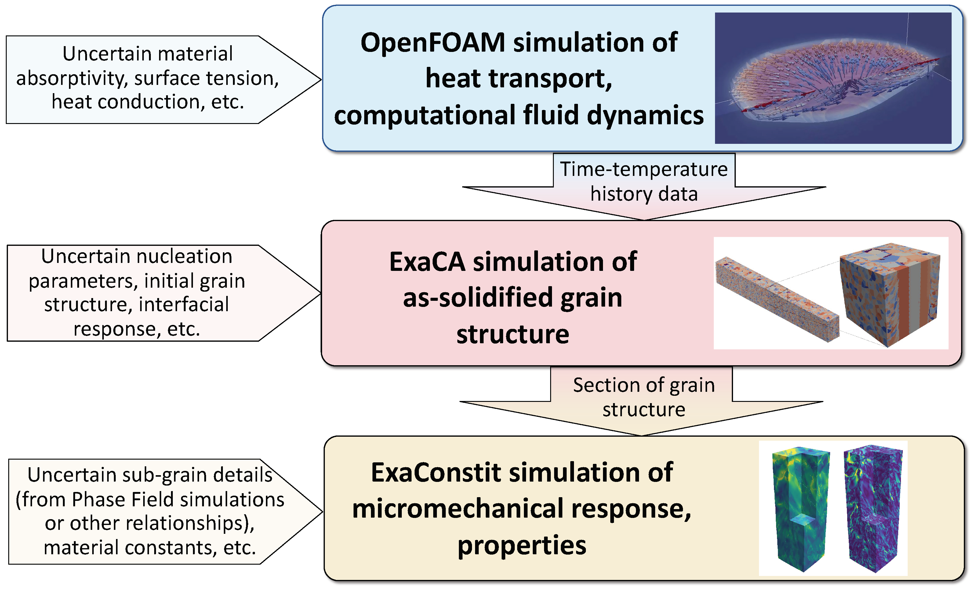
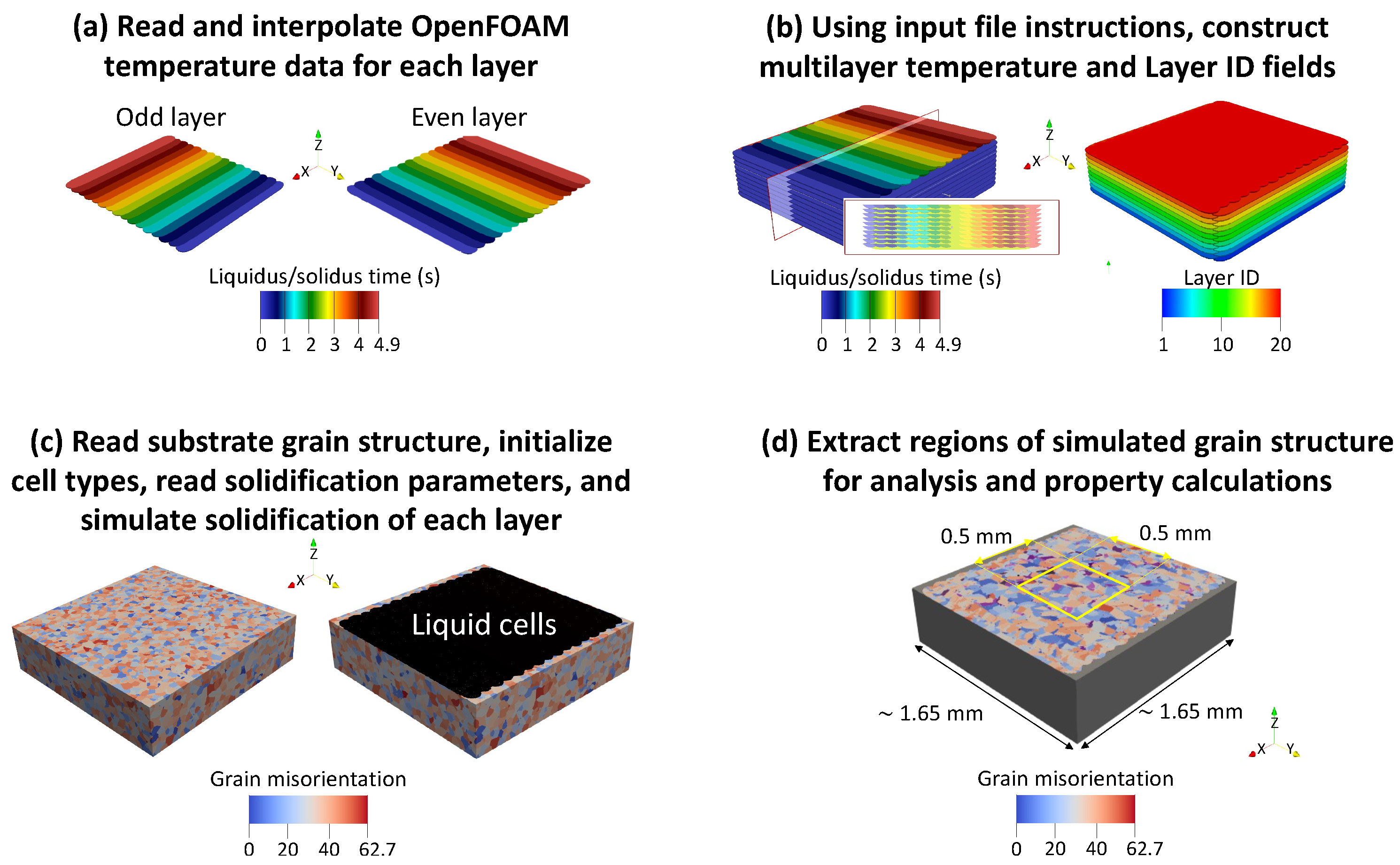
3.1. Workflow Description

An example of the workflow used to generate microstructure results is shown in Figure 2. Temperature input data were generated using a custom application developed using the OpenFOAM computational fluid dynamic platform to simulate heat and mass transfer in welding and additive manufacturing; more details on this application are given in [24]. This data were generated for two raster scan patterns: an “odd” layer, with each pass by the heat source alternating between the positive and negative X directions, and an “even” layer, with each pass by the heat source alternating between the positive and negative Y directions. The scan and material parameters for the relevant material, Inconel 625, are given in

Table 1. Material and scan parameters used in the OpenFOAM model for liquid and solid Inconel 625. The temperature-dependent parameters were considered as constants beyond 2000 K.

Parameter	Value
Laser efficiency	31%
Laser power	195 W
Laser depth	4.899 × 10−5 m
Laser radius (Gaussian beam shape)	1.041 × 10−4 m
Laser velocity	0.8 m/s
Laser passes per layer	16
Laser line offset	100 $\mathsf{\mu }$m
Liquidus temperature	1620 K
Solidus temperature	1410 K
Thermal expansion coefficient for liquid	1.25 × 10−4 K−1
Dendrite arm spacing for drag force	1 $\mathsf{\mu }$m
Thermocapillary coefficient	−3.08 × 10−4 N/(m · K)
Solid and liquid density (function of T)	8603.74–0.68278·T kg/m3
Solid heat capacity	428.38 + 0.23638·T J/(kg·K)
Solid thermal conductivity	8.9164 + 0.014743·T W/(m·K)
Liquid heat capacity	725.74 J/(kg·K)
Liquid thermal conductivity	8.9164 + 0.014743·T W/(m·K)
Latent heat of fusion	217,540 J/kg
Dynamic viscosity	0.003032 kg/(m·s)
Reference density for buoyancy	7569.92 kg/m3
Reference temperature for buoyancy	1620 K
Spatial resolution of generated	5 $\mathsf{\mu }$m
liquidus/solidus time data

; the result for each layer is a series of melt tracks approximately 30 to 40 $\mathsf{\mu }$m deep and 150 to 175 $\mathsf{\mu }$m wide. As shown in Figure 2a, these temperature data are a “sparse” form of the full time-temperature history as previously described by [66], consisting of a list of Cartesian coordinates from the OpenFOAM simulation that went above the alloy liquidus temperature. These coordinates are given on a regular grid, alongside the times at which each coordinate went below the liquidus and solidus temperatures for the final time. A trilinear interpolation scheme is used to interpolate this liquidus and solidus time from the OpenFOAM grid spacing to the CA cell size. By using temperature data of this form, the CA implicitly makes the assumption that solidification from remelted boundaries has a negligible effect on microstructure, as only the final time that a given CA cell undergoes solidification is calculated. This assumption previously appeared valid for shallow melt pools and raster scan patterns resembling those used in this present work [66]. In addition to the interpolated liquidus and solidus time data, input values are required for the number of layers simulated, the ordering of the layers, and the offset in the Z (build) direction between layers. Unless otherwise mentioned, in the present work, we simulate 65 layers of alternating even and odd scan patterns, offset by 20 $\mathsf{\mu }$m in the build direction. Using the temperature data and multilayer input values, a multilayer field of liquidus and solidus time values can be assembled. This assembly is schematically illustrated in Figure 2b. Temperature data from older layers are overwritten with data from newer layers, as only the final time that a given CA cell undergoes solidification is calculated. A field of “layer ID” values lists the layer during which each cell solidifies; since liquidus and solidus time values start at zero for each layer, linking the solidus and liquidus data with the appropriate layer is necessary.

Once the OpenFOAM data has been read and initialized by ExaCA, a substrate grain structure must be generated. This was performed using ExaCA itself as a preprocessing step to generate a “baseplate” microstructure as shown in Figure 2c: initializing an appropriately sized simulation domain of liquid cells, calculating the probability that a given cell of size $∆x$ will be the center of a baseplate grain based on an input mean substrate grain diameter $S_0$, and generating a random number $R_{substrate}$ between 0 and 1 for each cell. For cells where the condition

$$R_{substrate}<\frac{{∆x}^3}{{S_0}^3}$$

(1)

is satisfied, randomly oriented grain seeds (each grain has one of 10,000 possible random orientations) are placed at these sites. The model described in Section 3.2 is then used to let these grains growth at a constant rate until all liquid cells are claimed by a grain.

After reading in the appropriate OpenFOAM and substrate data for a given run, ExaCA will also read an input data file containing cell size, time step, and parameters governing nucleation and growth; these parameters and their use will be discussed in the following section. Finally, after the completion of an ExaCA simulation, a region 0.5 mm in the X and Y directions is taken from the center of the resulting microstructure for use in grain statistics calculation (shown schematically in Figure 2d and described further in Section 3.3) and properties analysis (described further in Section 3.4).

3.2. CA Model Description

The computational domain is divided into a regular grid of cells, with spacing $∆x$. A time step, $∆t$, is selected and used to convert the “liquidus time” data into values of “critical time step”, i.e., the time step at which a cell goes below the liquidus temperature for the final time. The difference between the liquidus and solidus times and temperatures is used together with $∆t$ to define an “undercooling change” value, or the rate at which the magnitude of the undercooling increases each time step following the “critical time step”, at which the cell has zero undercooling. Cells that do not have liquidus and solidus time data are part of the substrate, and are initialized as solid type. Cells that have liquidus and solidus time data are part of the melt pool and initialized as liquid type, with the exception of those that border solid cells that are initialized as active type. The cell undercooling is only tracked for active and liquid type cells, and only proceeding each cell’s critical time step (at which the undercooling is set to 0, and decremented by the cell’s undercooling change value each time step). Cells initialized as solid or active type have a grain ID value taken from the substrate input file, where each grain ID corresponds to an orientation taken from a list of 10,000 possible random orientations for the FCC Inconel 625 crystal structure.

The CA algorithm uses a series of rules associated with specific cell types to advance the system state each time step. The main set of rules relates to tracking the solidification front inside of undercooled active cells, which represent the solid–liquid interface, and the “capture” of adjacent liquid cells by grains associated with active cells. The decentered octahedron method, originally published by Gandin and Rappaz [39] and briefly summarized here, is used to model these grain growth and cell capture processes. The decentered octahedron method ensures that grain growth, regardless of grain orientation, is independent of the Cartesian grid directions. All active cells are initialized with associated octahedra, with the six-half diagonal directions of each octahedron aligned with the <001> directions of each cell’s grain orientation. These octahedra represent the grain envelopes, containing cellular or dendritic morphologies that the present model does not explicitly simulate. All octahedra are tracked independently from one another, even those belonging to the same parent grain ID. When the time step exceeds an active cell’s critical time step, the dimensionless size of said active cell’s octahedron, L, is increased by an increment

$$∆L=\frac{∆t}{∆x}(A(∆T){}^3+B(∆T){}^2+C(∆T)).$$

(2)

each time step based on the local undercooling in the cell, $∆T$. This interfacial response function links the local cell undercooling to the dimensionless dendrite growth velocity (in turn dependent on subscale phenomena such as solute diffusion and interfacial energy) and the expansion of the grain envelope. The polynomial form of the interfacial response function shown in Equation (2) and the associated constants A, B, and C are taken from a previously modeled nickel-based alloy [41], which in turn was chosen based on the interfacial response function calculated for pure nickel [67] and adjusted to match experimental grain structure data. As each active cell’s octahedron grows, any liquid cell adjacent to the active cell may become “captured” when the octahedron engulfs the liquid cell center. The liquid cell then becomes an active cell, becomes a member of the original active cell’s grain, and is given its own octahedron with the same orientation as the original active cell’s octahedron. The placement of octahedra centers, the initial size of new octahedra, and the geometry calculations involved in the cell capture process are provided in the original work on the decentered octahedron algorithm [39]. The max size of $∆L$ in Equation (2) is capped at 0.05 to avoid octahedron growth so rapid that the grain growth becomes dependent on the code’s iteration order through active cells. When an active cell no longer has any liquid neighbors, it becomes a solid cell, and its octahedron is no longer tracked. This process is repeated until all liquid cells associated with a given layer ID have been converted to active or solid cells, after which simulation of the next layer ID begins.

Heterogeneous nucleation in the CA model is governed by a nucleation density $N_0$, a mean nucleation undercooling $∆T_N$, and a standard deviation of the nucleation undercooling $∆T_{\sigma }$. This is performed in a slightly simplified manner as in the literature due to the simplifying assumptions of [66]: it is known a priori which cells will undergo solidification, and that each of these cells will only solidify once (intermediate remelting and solidification events are neglected). At the beginning of the simulation, a random number $R_{nucleation}$ between 0 and 1 is generated for each liquid cell. If the condition

$$R_{nucleation}<N_0{(∆x)}^3$$

(3)

is satisfied, the liquid cell is considered a potential nucleus site. Each potential nucleus is randomly assigned a nucleation undercooling value, taken from a Gaussian distribution with a mean of $∆T_N$ and standard deviation of $∆T_{\sigma }$. The potential nucleus will either become extinct if the liquid cell is captured by an adjacent active cell prior to reaching its assigned nucleation undercooling, or successfully become a nucleus if it remains liquid type upon reaching its assigned nucleation undercooling. If the nucleation event is successful, the cell becomes a new active cell, becomes part of a new grain, and is assigned an octahedron which will grow via the previously discussed decentered octahedron algorithm.

The values used for all CA model parameters are given in

Table 2. Default values for CA model parameters considered in the present work.

Parameter	Symbol	Value
Cell size	$∆x$	1.666 $\mathsf{\mu }$m
Time step	$∆t$	0.083 $\mathsf{\mu }$s
Interfacial response fitting parameter 3rd order	A	−1.0302 × 10−7 m/(s · K3)
Interfacial response fitting parameter 2nd order	B	1.0533 × 10−4 m/(s · K2)
Interfacial response fitting parameter 1st order	C	2.2196 × 10−3 m/(s · K)
Heterogeneous nucleation density	$N_0$	1013/m3
Mean nucleation undercooling	$∆T_N$	5 K
Standard deviation of nucleation undercooling	$∆T_{\sigma }$	0.5 K
Mean substrate grain diameter	$S_0$	45 $\mathsf{\mu }$m
Offset in build direction for new layers	None	20 $\mathsf{\mu }$m
Number of layers simulated	None	65

. These are used unless otherwise mentioned—notably, the heterogeneous nucleation density $N_0$ and mean substrate grain diameter $S_0$ will later be varied from their default values to examine their roles on microstructure development. As a brief aside, the CA cell size of 1.666 $\mathsf{\mu }$m is one third of the OpenFOAM data resolution of 5 $\mathsf{\mu }$m. A previous study using OpenFOAM data at 5 $\mathsf{\mu }$m resolution and various ExaCA $∆x$ using similar scan parameters found that this was the largest cell size able to achieve reasonably converged grain shape results [66]. For a general set of scan parameters, CA cell size and temperature field resolution required to fully resolve texture are unknown; however, cell sizes on the order of microns generally appear able to capture texture evolution in AM melt pool solidification [68]. Cell sizes on the order of microns are also more than an order of magnitude smaller than most AM part feature sizes (for example, the thin open cellular structure shown by [2] has internal support bars on the order of 10 s of microns), which should allow future work modeling grain structure in fine geometries in addition to bulk parts.

3.3. CA Data Analysis

To quantify the change in grain structure as a function of distance from the domain’s bottom surface (i.e., how the grain structure changes as a function of deposited layer), we introduce two parameters: a mean grain cross-sectional area $\varsigma$, and a mean weighted grain cross-sectional area $\overline{\varsigma }$. Using the entire domain cross-section for calculation of these parameters would skew the means via inclusion of substrate grains at and beyond the lateral bounds of the melted region, so we instead define an area in X and Y that is expected to be representative of the grain structure far from the scan edges. In the case of the even and odd layer scan patterns simulated through OpenFOAM, we select the 0.5 by 0.5 mm region (area of 0.25 mm², see yellow outline in Figure 2d) furthest from the boundaries for analysis. With a cell size of 1.666 $\mathsf{\mu }$m, this region is 300 cells wide in the X and Y directions. At a given Z coordinate within this representative area, the mean grain cross-sectional area is given by

$$\varsigma =\frac{0.25{\mathrm{mm}}^2}{N_G},$$

(4)

where $N_G$ is the number of unique grain ID values represented at the Z coordinate of interest. As many AM microstructures are dominated by a small number of grains with large cross-sectional areas, using a simple average of grain cross-sectional areas can skew small if many small grains are present. We introduce a weighted mean grain cross-sectional area for this reason, defined as

$$\varsigma =\frac{1}{0.25{\mathrm{mm}}^2}\sum _{i=1}^{i=N_G}{A_i}^2.$$

(5)

In Equation (5), the “weights” are the grain areas themselves, as $A_i$ is the cross-sectional area of a grain with grain ID “i”. Multiplying each $A_i$ by itself in Equation (5) in turn weights the average toward the areas of the largest grains. Paraview images of the resulting grain structure provide a qualitative way to examine ExaCA results. Two different colormaps are used in these Paraview images, one for grains that were originally part of the substrate, and one for grains that formed via heterogeneous nucleation events. The colormaps describe grains’ misorientation relative to the positive Z (build) direction, that is, the difference in angle between the positive Z direction and the closest aligned <001> direction for the grain orientation, which can range from 0 to 62.8 degrees based on crystal geometry [69].

Regions of grain structure are printed for use by ExaConstit in property calculations, in a format listing cell X, Y, Z, and grain ID values (with a corresponding file mapping each grain ID to one of the possible 10,000 random orientations). These representative microstructure regions are 300 by 300 by 300 CA cells in size, using the same 300 by 300 area in X and Y from the mean grain area calculations. Two separate 300 cell regions in the Z direction are selected, a “lower” region consisting of Z coordinates 170 through 469 (roughly corresponding to layers 15 through 39), and an “upper” region consisting of Z coordinates 470 through 769 (roughly corresponding to layers 40 through 64). The microstructure from the first 14 layers is excluded from these representative volumes as it is expected to skew towards the random texture and grain size of the substrate, and the final (65th) layer is excluded as the final layer of a build is well-known as being unrepresentative of the grain structure as a whole. In addition to comparing properties of grain structures with different $S_0$ and $N_0$, upper and lower regions are compared to quantify property variation in different spatial locations of the build.

3.4. Crystal Plasticity Model

In order to run the crystal plasticity simulations, we rely on three open source libraries. The crystal plasticity constitutive response is provided by the ExaCMech library [70] and then fed into ExaConstit to solve for the bodies response to an applied load. ExaConstit [26] is a general quasistatic nonlinear solid mechanics velocity-based finite element application built on the MFEM framework [71]. ExaConstit solves for the balance of linear momentum as given in Equation (6) using typical solid mechanics FEM discritizations of the weak form for nonlinear materials.

$$\nabla ·\sigma =0$$

(6)

ExaCMech provides a number of different elastoviscoplastic crystal plasticity models available to the user. These models all employ large strain kinematics with varying crystal-scale constitutive responses for the elastic and plastic response. A detailed description of these sorts of models can found in [72,73]. A brief description of the kinematics and constitutive response of the material will be described here. Starting from the velocity gradient, $\mathbf{L}$, we can decompose the kinematic response into the following:

$$\mathbf{L}=\dot{\mathbf{F}}{\mathbf{F}}^{-1}={\dot{\mathbf{V}}}^e{\mathbf{V}}^{e-1}+{\mathbf{V}}^e{\widehat{\mathbf{L}}}^p{\mathbf{V}}^{e-1}$$

(7)

where $\mathbf{F}$ is the deformation gradient, ${\mathbf{V}}^e$ is the elastic left stretch tensor, and ${\widehat{\mathbf{L}}}^p$ is defined as:

$${\widehat{\mathbf{L}}}^p={\dot{\mathbf{R}}}^{*}{\mathbf{R}}^{*T}+{\mathbf{R}}^{*}{\dot{\mathbf{F}}}^p{\mathbf{F}}^{p-1}{\mathbf{R}}^{*T}$$

(8)

where ${\mathbf{R}}^{*}$ is the lattice rotation and ${\mathbf{F}}^p$ is the plastic deformation gradient. The plastic velocity gradient, ${\overline{\mathbf{L}}}^p={\dot{\mathbf{F}}}^p{\mathbf{F}}^{p-1}$, appearing in Equation (8) is directly related to the combined macroscopic shearing of the slip systems:

$${\overline{\mathbf{L}}}^p=\sum _{\alpha =1}^n{\dot{\gamma }}^{\alpha }{\overline{\mathbf{s}}}^{\alpha }\otimes {\overline{\mathbf{m}}}^{\alpha }$$

(9)

where ${\dot{\gamma }}^{\alpha }$ is the plastic shearing rate on the $\alpha$ slip system and ${\overline{\mathbf{s}}}^{\alpha }\otimes {\overline{\mathbf{m}}}^{\alpha }$ is the Schmid tensor defined in the crystal reference frame. Our plastic shearing rate is described by our choice of models for our slip kinetics and hardening models. For this study, we make use of a power law slip kinetics formulation with a Voce hardening model. Our slip kinetics takes on the following form:

$${\dot{\gamma }}^{\alpha }={\dot{\gamma }}_0{\left(\frac{{\tau }^{\alpha }}{g^{\alpha }}\right)}^{\frac{1}{m}}\mathrm{sgn}\left({\tau }^{\alpha }\right)$$

(10)

where ${\dot{\gamma }}_0$ is a reference shearing rate, ${\tau }^{\alpha }$ is a resolved shear stress on the $\alpha$ slip system, $g^{\alpha }$ is the critically resolved shear strength on the $\alpha$ slip system, and m is the rate sensitivity of slip. The resolved shear stress can be computed as the following:

$${\tau }^{\alpha }=\sigma :{({\widehat{\mathbf{s}}}^{\alpha }\otimes {\widehat{\mathbf{m}}}^{\alpha })}_{sym}$$

(11)

where $\sigma$ is the Cauchy stress. We describe $g^{\alpha }$ using a Voce hardening model as defined below:

$${\dot{g}}^{\alpha }=h_0\left(\frac{g_{sat}-g^{\alpha }}{g_{sat}-g_0^{\alpha }}\right)\sum _{\beta =1}^{n_{slip}}{\dot{\gamma }}_{\beta }$$

(12)

where $h_0$ is the strength hardening coefficient, $g_0$ is the initial critically resolved shear strength, and $g_{sat}$ is the saturation critically resolved shear strength.

The crystal elastic moduli for the Inconel 625 used in the simulations are listed in

Table 3. Single crystal elastic constants (Inconel 625) employed in simulation, along with the elastoviscoplastic model constants used for Inconel 625.

Parameter	Value
$C_{11}$	243.3 GPa
$C_{12}$	156.7 GPa
$C_{44}$	117.8 GPa
$h_0$	791.0 MPa
$g_0$	328.5 MPa
$g_{sat}$	788.0 MPa
m	0.03
$m^{\prime }$	0.0
${\dot{\gamma }}_0$	1.0 s−1
${\dot{\gamma }}_{s0}$	$5\times {10}^{10}$ s−1

along with the slip system parameters. The elastic moduli were taken from [74]. The choice of elastoviscoplastic model parameters are based upon stress–strain data obtained from the stress-relieved AM Inconel 625 in [75].

4. Results

4.1. Baseline Uncertainty in CA Microstructures

To quantify the variation in grain structure as a function of the number of deposited layers, a baseline for the spread in grain area statistics based on the two significant sources of “randomness” in ExaCA needs to be established. First, we set the mean substrate grain diameter $S_0$ and heterogeneous nucleation density $N_0$ to the default values from Table 2. The first source of randomness is the random number generator seed used to generate substrate grain orientations and locations, i.e., the seed used in generation of $R_{substrate}$ values used in the comparison from Equation (1). The second source of uncertainty is the random number generator seed used to generate heterogeneous nuclei locations, i.e., $R_{nucleation}$ values used in the comparison from Equation (3), and their associated activation undercooling values. Three different random number generator seeds are used for each of these two sources of uncertainty, generating three statistically equivalent substrates and three statistically equivalent sets of nucleation sites. The nine possible permutations of these seeds are used in simulation initialization, and the resulting mean grain cross-sectional area ($\varsigma$) and weighed mean cross-sectional area ($\overline{{\varsigma }_W}$) as a function of build height are shown in Figure 3 and Figure 4, respectively. As the curves in Figure 3 are similar and have a degree of noise, $\varsigma$ values are plotted as a moving average with a period of 25 data points (41.666 $\mathsf{\mu }$m) for curve visibility.

For all substrates and nucleation seeds, three regimes are seen in Figure 3 as a function of distance from the bottom surface: a sharp drop in $\varsigma$, a steady and slowly flattening increase in $\varsigma$, and a final sharp drop in $\varsigma$ (partially obscured as $\varsigma$ is plotted as a moving average). The two drops are related to nucleation of grains during simulation of the first few layers and the final layer, while the increase is related to the quasisteady-state nucleation and impingement of less favorably oriented grains occurring during the successive simulation of each new layer. Unlike the plot of $\varsigma$, the plot of $\overline{\varsigma }$ in Figure 4 does not show the initial transient nor final transient decrease—by weighting the largest grains more heavily in the average, a smoother, less noisy description of the dominant microstructural features is obtained. The increases in $\varsigma$ and $\overline{\varsigma }$ flattened off significantly after the first 600 $\mathsf{\mu }$m (30 layers or so), and even more after the first 1000 $\mathsf{\mu }$m, though it is not clear that the grain areas have reached a steady state with respect to build height even after all 65 layers. Additionally, the increase in $\overline{\varsigma }$ toward the steady state in Figure 4 appears to be happening more slowly than the corresponding $\varsigma \left(z\right)$ curves in Figure 3.

The spread in $\varsigma$ due to random substrate and nucleation seed increases as a function of build height through the first 250 $\mathsf{\mu }$m of solidification, beyond which there is approximately a ±150 $\mathsf{\mu }$m² or ±7% variation from the mean across all substrates and nucleation seeds. The spread in $\overline{\varsigma }$ due to random substrate and nucleation seed increases as a function of build height through the first 500 $\mathsf{\mu }$m of solidification, beyond which there is approximately a ±500 $\mathsf{\mu }$m² or around ±8% variation from the mean value. Neither nucleation seed nor substrate seems to be the dominant factor in the randomness of the grain area data: we do not see clustering of colors (which would indicate that substrate controls the scatter), nor do we see clustering of line types (which would indicate that nucleation seed controls the scatter).

4.2. CA Predictions with Varied Mean Substrate Grain Diameter

Now that the development of $\varsigma$ and $\overline{\varsigma }$ as a function of build height and random seeds have been quantified, we examine the effect of varied mean substrate grain size $S_0$ on microstructure far from the substrate. We generate five substrates with $S_0$ values ranging from 25 to 65 $\mathsf{\mu }$m as reasonable guesses for AM baseplate grain sizes. $\varsigma$ and $\overline{\varsigma }$ as a function of distance from the bottom build surface starting from these varied initial conditions are shown in Figure 5 and Figure 6, respectively.

As shown in Figure 5, after approximately 600 $\mathsf{\mu }$m (20–25 layers), $\varsigma$ for all substrates is within 20% of its “final” (after all 65 layers) value. After 65 layers of simulation for all substrates, there is a mean grain area spread of around 250 $\mathsf{\mu }$m², a spread similar to the scatter in $\varsigma$ induced through random number variation in the model from Section 4.1. For the three smaller $S_0$ values, $\varsigma$ shows more of a true convergence, as the curves for $\varsigma \left(z\right)$ with $S_0$ < 55 $\mathsf{\mu }$m are mostly indistinguishable after 65 layers. However, the $S_0$ = 55 and 65 $\mathsf{\mu }$m curves remain distinct from the $S_0$ = 25, 35, and 45 $\mathsf{\mu }$m curves. In Figure 6, the $\overline{\varsigma }$ curves show a less clear trend in convergence as a function of distance from the bottom surface, for all substrate grain diameters but particularly $S_0$ = 55 and 65 $\mathsf{\mu }$m. After 65 layers of simulation, a $\overline{\varsigma }$ spread of around 3000 $\mathsf{\mu }$m² is present as a function of $S_0$—a spread more significant than that induced through statistical variation in substrate/nucleation random seed alone (which was closer to 500 $\mathsf{\mu }$m² as shown in Section 4.1).

The difference in mean grain area and mean weighted grain area development among small and large $S_0$ simulations can be rationalized as a result of the two types of competition: that among the baseplate grains, and that between baseplate and nucleated grains. For small $S_0$, favorably oriented grains impinge less favorably oriented baseplate grains relatively quickly during the initial transient layers. However, with large $S_0$, there are fewer baseplate grains and impingement is less likely. For large $S_0$, grains unfavorably oriented with the local thermal gradient direction are therefore more likely to advance due to this lack of competition. In this case, nucleation and growth of new grains (some of which will have more favorable orientations than adjacent epitaxial grains) is the only other mechanism for impinging the less favorably oriented grains. This process is more likely with large $S_0$, as advancing baseplate grains with unfavorable orientation relative to the local thermal gradient direction require larger undercooling to advance in said direction. This larger undercooling provides the opportunity for nucleated grains to grow despite the large thermal gradient magnitude that would normally suppress nucleated grain growth. However, this process of baseplate grain impingement via growing nucleated grains takes many more layers to occur as heterogeneous nucleation of more favorably oriented grains is relatively rare, and the large magnitude of G present at the melt pool boundary still tends to suppress growth of nucleated grains. This explains why the decrease in $\varsigma \left(z\right)$ and $\overline{\varsigma }\left(z\right)$ for $S_0$ = 55 and 65 $\mathsf{\mu }$m in Figure 5 and Figure 6 toward the other curves is much more gradual than the initial transient increase in $\varsigma \left(z\right)$ and $\overline{\varsigma }\left(z\right)$ seen for the $S_0$ = 25, 35, and 45 $\mathsf{\mu }$m curves.

This conclusion is supported by Figure 7, which plots the interior region (away from the scan edges) of the simulated grain structure colored by grain source (baseplate or nucleation) and grain misorientation. It is shown that while high aspect ratio columnar grains of relatively similar area are present for $S_0$ = 25 and 65 $\mathsf{\mu }$m simulations, the larger $S_0$ simulation volume appears to have more nucleated grains (shades of red), particularly toward the top surface. Figure 8 also supports this conclusion; it shows the 001 pole figures using data from the top halves of the volumes from Figure 7 plotted using the MTEX toolbox. For all $S_0$, a reasonably strong (2–3x a uniform random distribution) 001 texture is observed, along with a secondary near-110 texture. However, these also show that the 001 texture is slightly weaker as $S_0$ is increased (lighter shades of green/yellow), and the regions of the pole figure corresponding to unfavorable orientations show slightly increased intensity (lighter shades of gray). This likely corresponds to both unfavorably oriented baseplate grains as well as nucleated grains, as unfavorably oriented baseplate grains as well as nucleated grains (which will have random orientations, though the more favorably oriented nucleated grains would be expected to grow to the largest sizes) lead to a slight decrease in the overall texture. We also note that the tall grains extending through many layers observed in Figure 7 and the 001 textures observed in Figure 8 are commonly seen in simulated and experimental AM of Inconel alloys [18,21,44,60]. While the material and scan parameters used in the present simulation were not designed to reproduce a specific result from experiment, the similarity of the simulated result with other simulations and experimental grain structures validates the present set of simulated process and solidification model parameters as relevant to real AM processing.

4.3. CA Predictions with Varied Nucleation Density

The development of grain structure induced through varying heterogeneous nucleation density $N_0$ was calculated at multiple $S_0$ values to compare the relative importance of $N_0$ and $S_0$. For $S_0$ values of 25, 45, and 65 $\mathsf{\mu }$m, $\overline{\varsigma }\left(z\right)$ was calculated using $N_0$ = 10¹² m⁻³ and 10¹⁴ m⁻³, and compared to a the $N_0$ = 10¹³ m⁻³ results from Section 4.2. This is plotted in Figure 9, where different line colors are used for different $N_0$ and different line markers are used for different $S_0$. Purely epitaxial growth ($N_0$ = 0) for the intermediate substrate grain size $S_0$ = 45 $\mathsf{\mu }$m is also plotted alongside results for the other permutations of $N_0$ and $S_0$.

Convergence of $\overline{\varsigma }$ curves with varied $S_0$ is strongly dependent on $N_0$. The largest $N_0$ in Figure 9 (black) shows $\overline{\varsigma }$ with different substrates to be within 1000 $\mathsf{\mu }$m² after 500 $\mathsf{\mu }$m of build, while the smallest $N_0$ (red) shows little to no convergence of $\overline{\varsigma }$ (each substrate grain diameter’s curve “flattens out”, but at different values $\overline{\varsigma }$ values). The curve corresponding to purely epitaxial growth (purple dashes) is similar to the curve corresponding to the smallest $N_0$ of 10¹² m⁻³ (red dashes). Given that nearly entirely epitaxial solidification is unlikely during AM processing (otherwise, we would see grains spanning the entirety of parts), this nucleation density is likely on the small side. The slower convergence of $\overline{\varsigma }$ curves at smaller $N_0$ and faster convergence of $\overline{\varsigma }$ curves at larger $N_0$ is expected, as reaching a value of $\overline{\varsigma }$ independent of distance from the bottom surface depends on the balance of nucleation and impingement. Impingement is a slow process of baseplate grains blocking other baseplate grains as additional layers are deposited, while nucleation occurs in every layer and introduces new grains. The more new grains are introduced, the fewer layers are needed to reach the quasisteady-state balance of nucleation and impingement. The extreme condition with zero nucleation would be expected to take a large number of layers to reach the point where all impingement has occurred and $\overline{\varsigma }$ is independent of additional layer deposition, while the extreme condition with infinite nucleation would be expected to reach this point after a single layer, as all cells would be home to their own grain. As might be expected, $\overline{\varsigma }$ as a function of build height has a stronger dependence on the substrate grain structure when $N_0$ is small, as impingement of substrate grains via nucleation becomes less common.

Figure 10 shows sections of the grain structures for each $N_0$ value at the fixed $S_0$ of 45 $\mathsf{\mu }$m. As expected based on the minimal difference in Figure 9 between purely epitaxial growth (purple dashes) and the nucleation density of 10¹² m⁻³ (red dashes) for the 45 $\mathsf{\mu }$m substrate diameter, the 10¹² m⁻³ grain structure is almost entirely epitaxial grains, with a small handful of large nucleated grains. The 10¹⁴ m⁻³ grain structure, after the first 0.5 mm or so of the build, is around 50% nucleated grains. Figure 11 shows the 001 and 110 pole figures for the upper halves of the simulation volumes shown in Figure 10, showing that while the overall 001 texture is present in approximately equal magnitudes for all $N_0$, a stronger competing 110 texture is present in the $N_0$ = 10¹⁴ m⁻³ case. This is confirmed by Figure 10, as the largest nucleated grains tended to have misorientation angles relative to the build direction of around 45 degrees (i.e., 110 grain orientations); these 110 grains have tall, columnar shapes similar to the baseplate grains. It is possible that the 110 orientations favored by the largest nucleated grains are related to the local thermal gradient direction in regions of the melt pool favorable for nucleation and growth. The overall grain shape appeared relatively independent on $N_0$ as it did with $S_0$, with more narrow grain areas the primary difference as $N_0$ was increased.

4.4. ExaConstit Model of Constitutive Properties with Varied Mean Substrate Grain Diameter and Nucleation Density

Representative volume elements (RVEs) from the ExaCA simulations using $N_0$ = 10¹² and 10¹³ m⁻³ and $S_0$ = 25, 45, and 65 $\mathsf{\mu }$m were passed to ExaConstit to model their macroscopic behaviors for part scale predictions. The macroscopic stress–strain response and distribution of triaxiality will be examined in this study as they are of use in fitting macroscopic models for part scale predictions [76,77,78,79,80,81,82]. As discussed in Section 3.3, these RVEs consisted of cubes with 300 cells (0.5 $\mathsf{\mu }$m of material) per side, and two RVEs were extracted from each ExaCA simulation: an “upper” RVE corresponding to the top 24 layers of depositied material (excluding the final layer), and a “lower” RVE corresponding to the 24 layers of material below the upper sample. Given that $\varsigma$ and $\overline{\varsigma }$ evolution clearly depended on $N_0$ and $S_0$, crystallographic texture development as a function of build height may not be the same. This difference in texture would be expected to result in differences in ExaConstit’s macroscopic property predictions, particularly when comparing the lower (more influenced by the baseplate) and upper (less influenced by the baseplate) RVEs.

Simulations were carried out under uniaxial tension at $1\times {10}^{-3}{\mathrm{s}}^{-1}$ strain rates out to 5% strain. Figure 12 shows ExaConstit’s prediction for the stress–strain behavior of the various permutations of $S_0$, $N_0$, and RVE location in the build. As expected, the elastic response and plastic response of these RVEs are largely similar given similar grain morphologies and textures of each RVE. However, we do see differences in the yield stress and later responses in the fully-developed plastic flow areas of the curve. For example, the upper $S_0$ = 25 $\mathsf{\mu }$m, $N_0$ = 10¹² m⁻³ curve has the lowest yield stress and macroscopic stress response of the various RVEs. The lower $S_0$ = 65 $\mathsf{\mu }$m, $N_0$ = 10¹² m⁻³ RVE is on the other end of things and has the highest yield stress. To better compare differences in the response, we make use of a heat map to compare the relative percent difference between yield stresses of all samples. The percent differences in yield stress are plotted in Figure 13, and this figure shows that most samples are similar to one another. The yield stress for the upper $S_0$ = 25 $\mathsf{\mu }$m, $N_0$ = 10¹² m⁻³ is the biggest outlier, with a greater than a 5% difference in the response between this RVE and those using $S_0$ = 65 $\mathsf{\mu }$m. For the most part, these differences are largely due to nucleation or baseplate structures having different textures, and the differences are relatively minor. Other limiting factors on the material response, such as defects or pores in the solidified material or statistical variation in builds could play a larger role in an application needs.

To drive porosity-models at the part scale, distributions of the hydrostatic stress can be used to instantiate these models [83]. Rather than examining the hydrostatic stress, we will examine the stress triaxiality, which is defined as

$$Triaxiality=\frac{{\sigma }_h}{{\sigma }_{vm}},$$

(13)

where ${\sigma }_h$ is the hydrostatic stress and ${\sigma }_{vm}$ is the von Mises stress. Figure 14 shows the stress triaxiality distributions for the lower and upper RVEs of varied $N_0$ and $S_0$. These distributions are often used in the mechanics community to investigate potential areas with an increased likelihood of fracture. The width and maximum height of these distributions are nearly identical for all lower and upper RVEs, though it is noted that the lower $S_0$ = 65 $\mathsf{\mu }$m, $N_0$ = 10¹² m⁻³ and upper $S_0$ = 65 $\mathsf{\mu }$m, $N_0$ = 10¹³ m⁻³ distributions have long tails at small triaxiality. While these tails look significant on the histograms, we note that the y-axis counts are given on a log scale, and that the number of elements represented in these tails is relatively insignificant compared to the distribution peaks, which are similar for all RVEs. These tails likely consist of one or two anomalous grains, either from the baseplate or from a specific heterogeneous nucleation event.

4.5. CA Predictions Using Extremes in Substrate Initial Conditions

We can also examine grain structure development starting from the largest possible “extremes” in initial substrate. For the first extreme, we use a single grain as the substrate, selecting the orientation from the list of 10,000 with all axes as closely aligned with the <001> directions as possible. For the second extreme, a single grain is again used as the substrate, but the orientation with growth directions as misaligned as possible from the positive Z direction is selected from the list of 10,000 possible orientations. For the final extreme, each CA cell that is part of the substrate is assigned a different grain ID and orientation, essentially simulating a substrate grain size equivalent to the CA cell size.

Figure 15 shows the resulting grain structures after 120 layers of CA calculations. The top surfaces of the simulation domains show the grain shapes and sizes beginning to resemble those starting from the standard equiaxed substrates from Figure 7 and Figure 10. Starting from the single crystal substrates, nucleated grains partially block regions of the substrate from advancing and growth through multiple layers, though regions of the single crystal substrates are still visible at the top surface after 120 layers. The orientation of the single substrate grain plays a role in layerwise grain structure development as well, with more nucleated grains appearing and advancing after fewer layers with the large misorientation substrate, relative to the small misorientation substrate. This difference is due to the fact that the low misorientation substrate tends to be closer aligned with the thermal gradients in more regions of the melt pool, and therefore its growth is more competitive with nucleated grains (which are less likely to be as closely aligned with the local thermal gradients). The high misorientation grain is less likely to be closely aligned with the thermal gradient direction (as evidenced by the fact that misorientations greater than 45 degrees were rare in Figure 7 and Figure 10), and this high misorientation grain is less competitive with nucleated grains, which are therefore able to form and grow more readily. Large area nucleated grains extending through multiple layers are not as readily seen when starting from the extreme condition where each cell is its own grain. This is likely because with more substrate grains present, regions of the melt pool favorable for nucleation through large misalignment between the thermal gradient direction and substrate grain orientation are less common.

The textures of these simulations are also interesting to note; Figure 16 shows the 001 pole figures using the top 30 layers of the volumes shown in Figure 15. The $S_0$ = 45 $\mathsf{\mu }$m pole figure, reproduced from Figure 8, is also plotted for reference. For the low misorientation single grain substrate, the 001 texture is stubborn (likely due to the fact that it is strongly favored by the thermal conditions), though a weak competing 110 texture does appear through the growth of nucleated grains. For the high misorientation single crystal substrate, the 111 texture from the substrate is still visible in the pole figure, but reasonably strong 001 and 110 textures have also developed. Finally, when starting from the smallest possible grain size, 001 and 110 textures are visible with approximately the same intensity as the $S_0$ = 45 $\mathsf{\mu }$m pole figure, but other orientations such as 210 and 111 remain present as well. These results show that despite the relative insensitivity of texture to $S_0$ after 15+ layers observed in Section 4.2, reasonable initial conditions are still required to obtain a reasonable texture without the need to simulate several millimeters of build. However, we note that if these simulations were continued for thousands of layers, it is expected that even with disparate initial conditions, the microstructures far enough from the initial substrate would still be expected to become indistinguishable.

5. Discussion

The coupled modeling of process, microstructure, and properties were investigated using three codes that serve as part of the ExaAM framework for self-consistent modeling of AM processes. AM raster pattern time–temperature history from the computational fluid dynamics software OpenFOAM served as input to multilayer grain structure simulations with the cellular-automata-based ExaCA code. A series of ExaCA simulations were performed, with the main takeaways as follows:

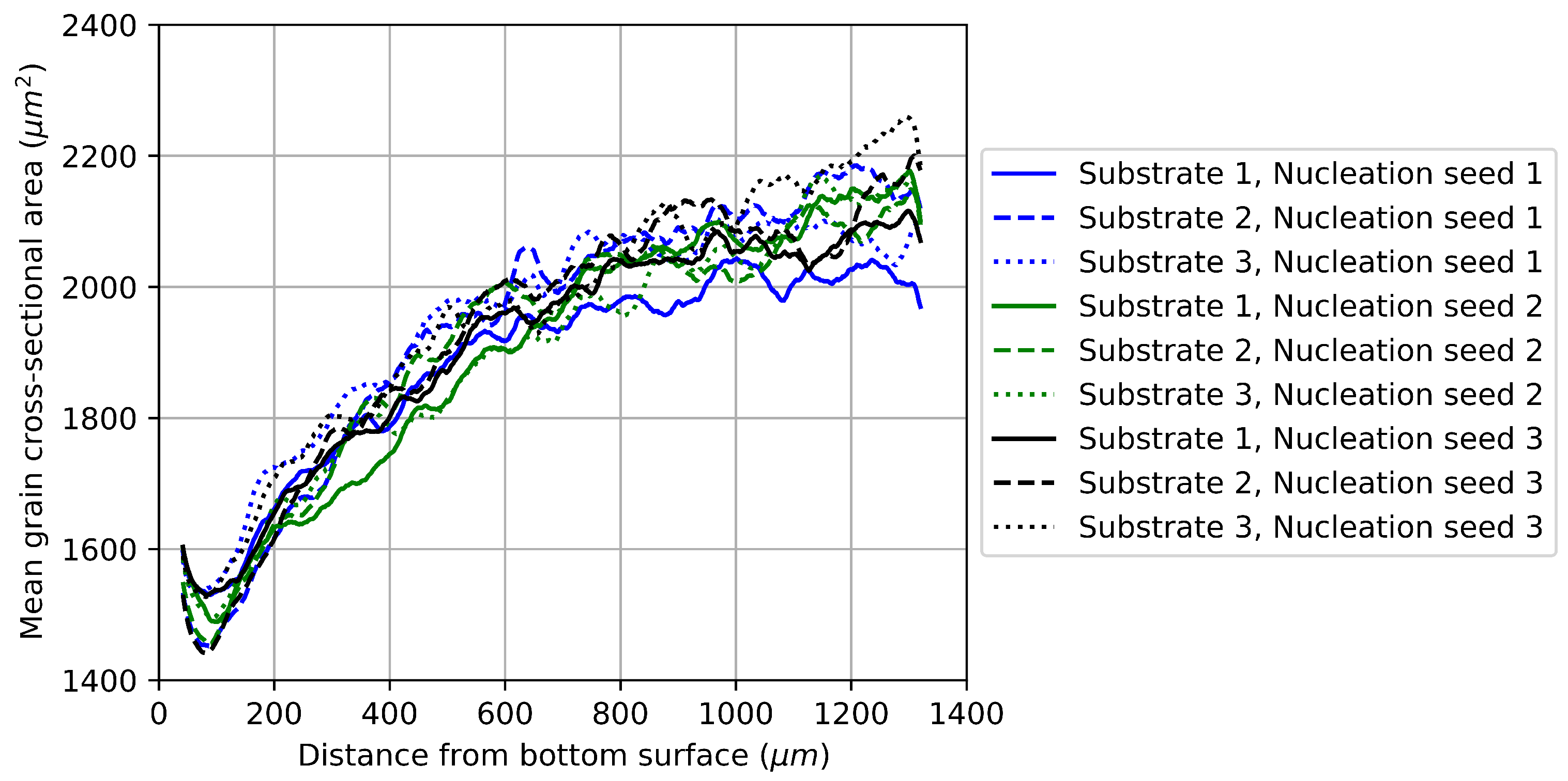
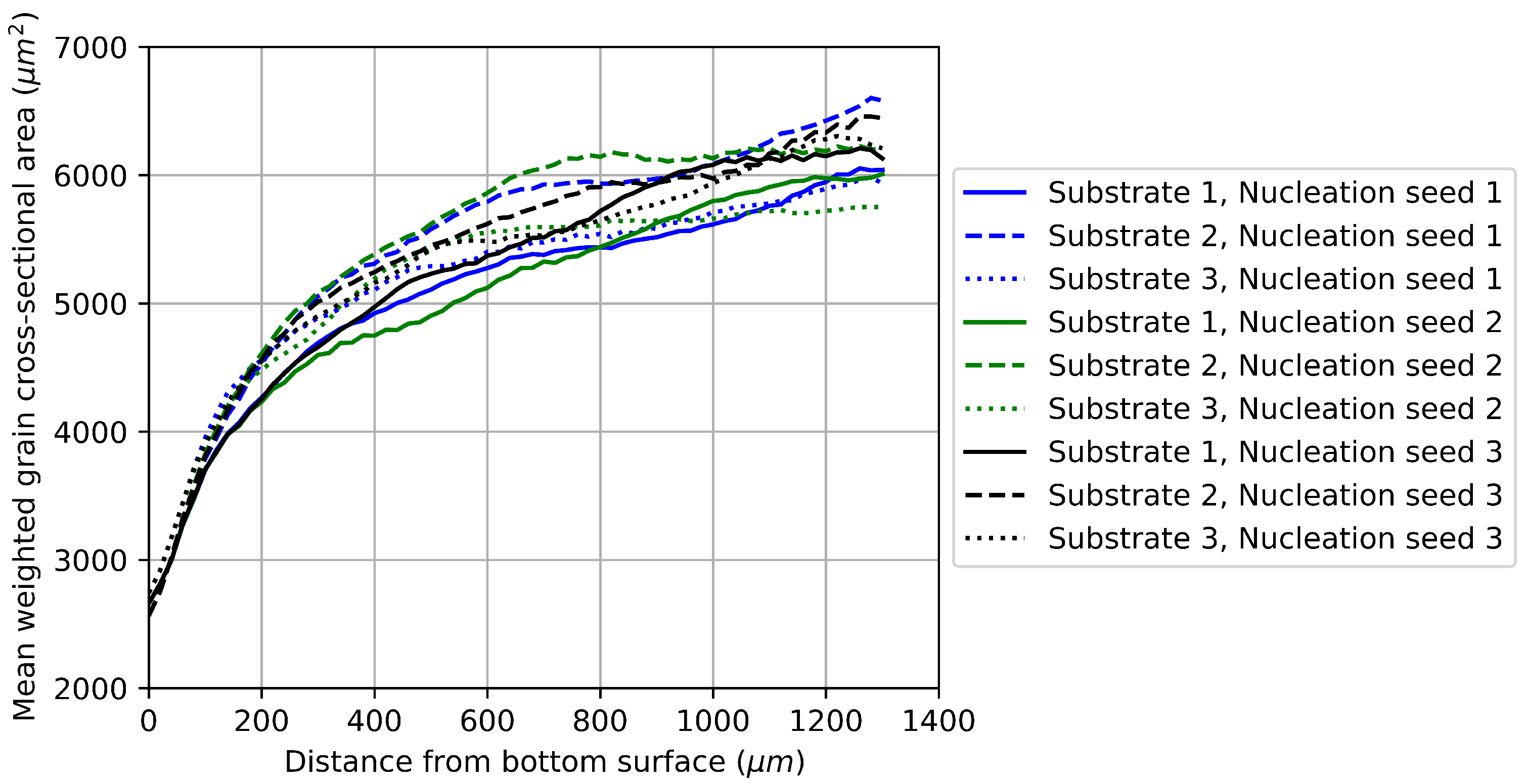
• Mean grain area ($\varsigma$) as a function of build height (z) was plotted for fixed nucleation density and substrate, while varying the random number generator seeds used to generate statistically equivalent sets of nucleation and substrate data. The resulting $\varsigma \left(z\right)$ curves slowly became independent of additional layer deposition (i.e., z), with spreads in the steady-state $\varsigma \left(z\right)$ values of 7%–8% from statistical error due to the random number generation processes. The same was true for mean weighted grain area ($\overline{\varsigma }$).
• Statistical error resulting from substrate generation and nucleation data generation appeared to contribute to the spread in predicted $\varsigma$ and $\overline{\varsigma }$ equally. The average of the $\varsigma$ curves was within 10% of its 65 layer value, and the average of the $\overline{\varsigma }$ curves was within 15% of its 65 layer value, after around 500 $\mathsf{\mu }$m of build (or about 23 layers).
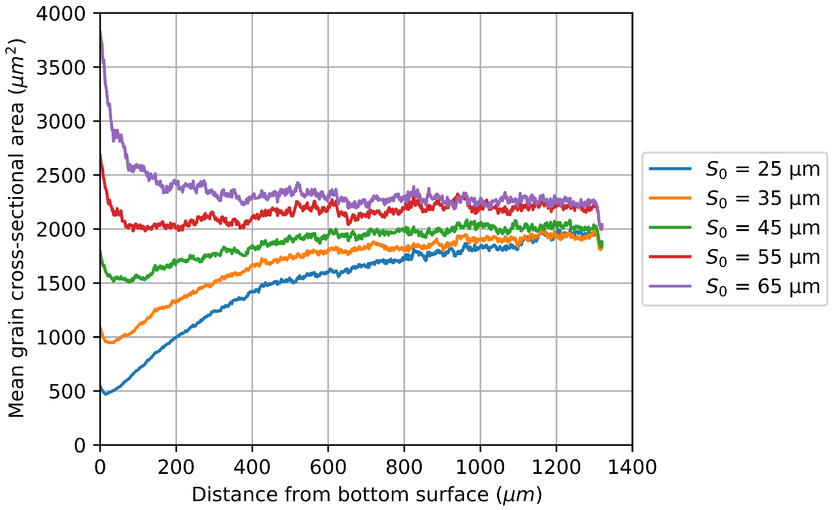
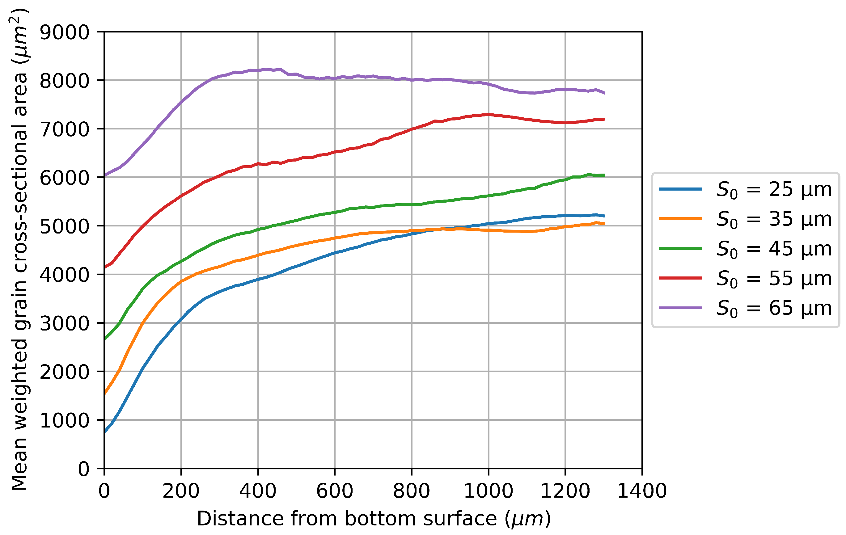
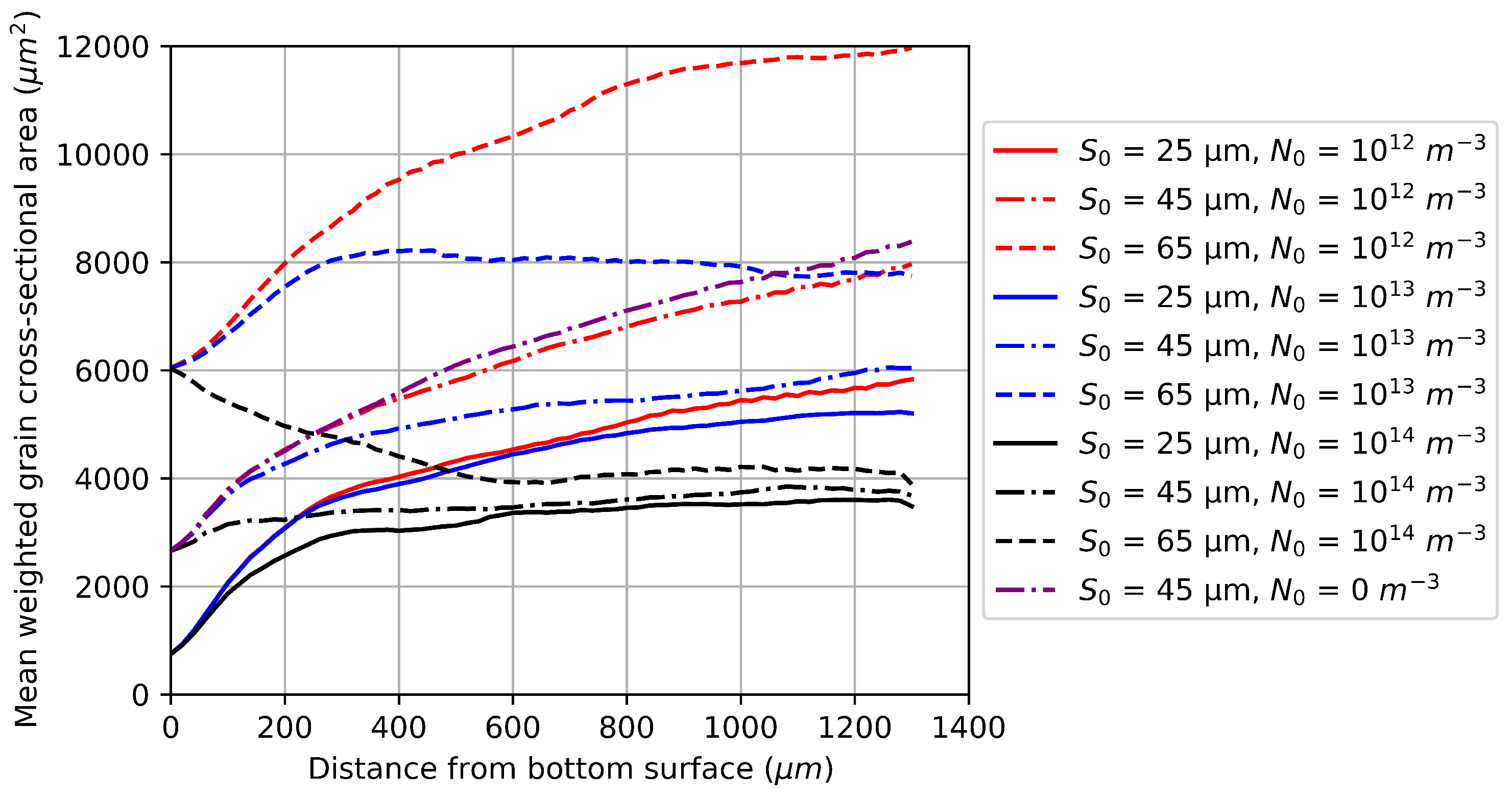
• Examining $\varsigma$ and $\overline{\varsigma }$ curves with ±20 $\mathsf{\mu }$m from the default mean substrate grain diameter $S_0$ = 45 $\mathsf{\mu }$m, it was found that curves with smaller $S_0$ tended to converge more quickly than those at larger $S_0$, and reach steady-state values more quickly than those at larger $S_0$. The spread of these curves with $S_0$ > 45 $\mathsf{\mu }$m after 1.2 mm of simulated build remained significant relative to the uncertainty in $\varsigma \left(z\right)$ and $\overline{\varsigma \left(z\right)}$ due to random number generation alone.
• Steady-state values of $\overline{\varsigma }$ as a function of z were much more readily reached at large $N_0$, regardless of $S_0$; at $N_0$ = 10¹⁴ m⁻³, this steady state appeared to be reached after 0.6 mm of simulated microstructure. As $N_0$ was reduced to 10¹² m⁻³, $S_0$ had a much larger impact on the $\overline{\varsigma }\left(z\right)$ curves, and $\overline{\varsigma }$ was still increasing as a function of z after 1.2 mm of simulated microstructure.
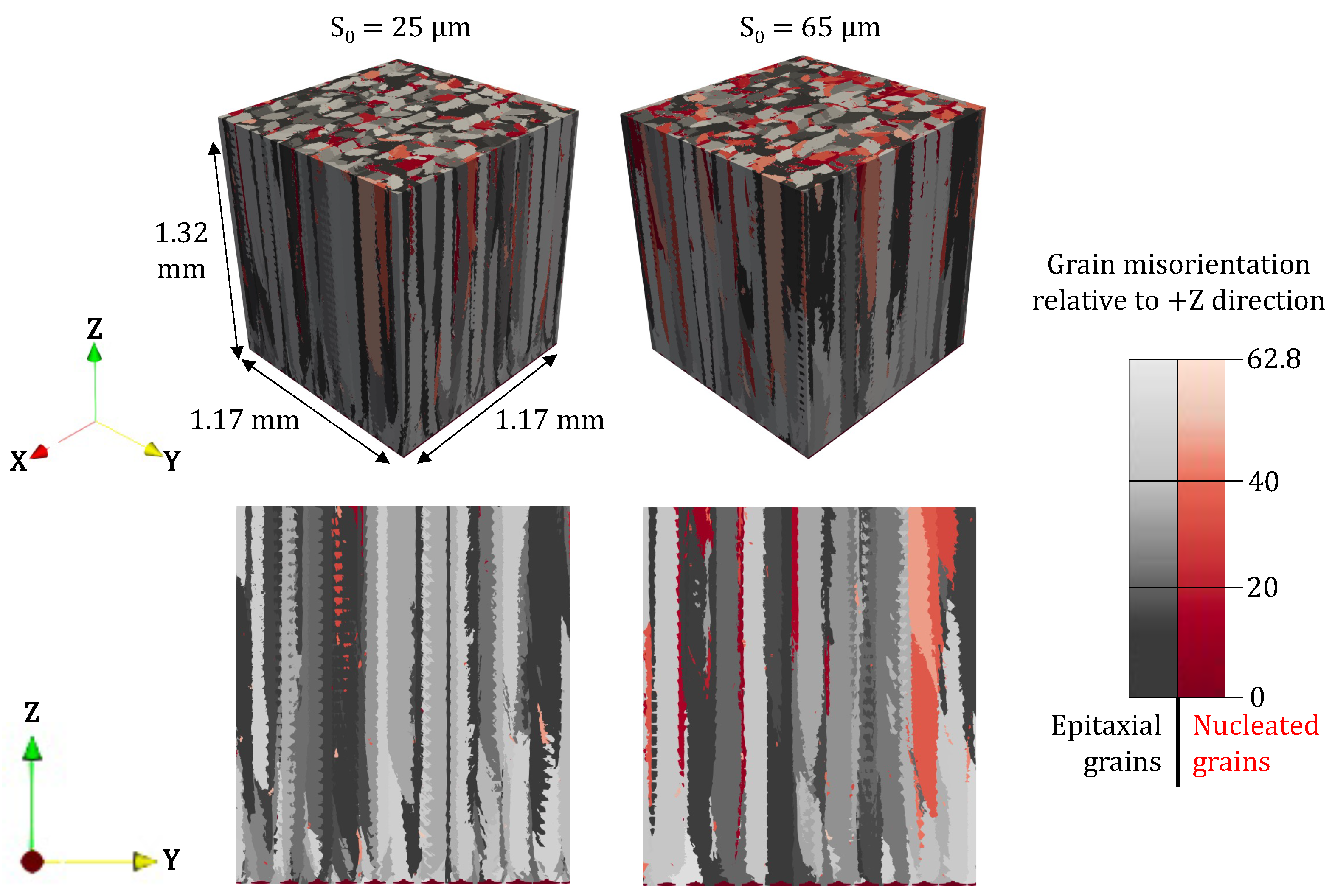
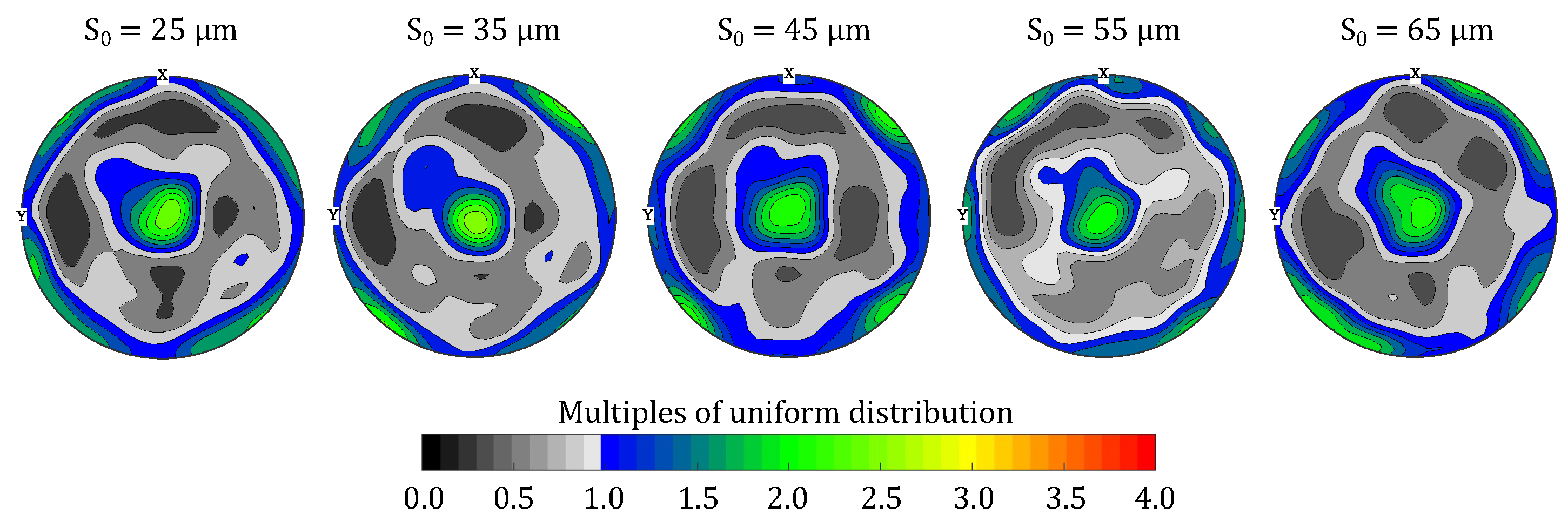
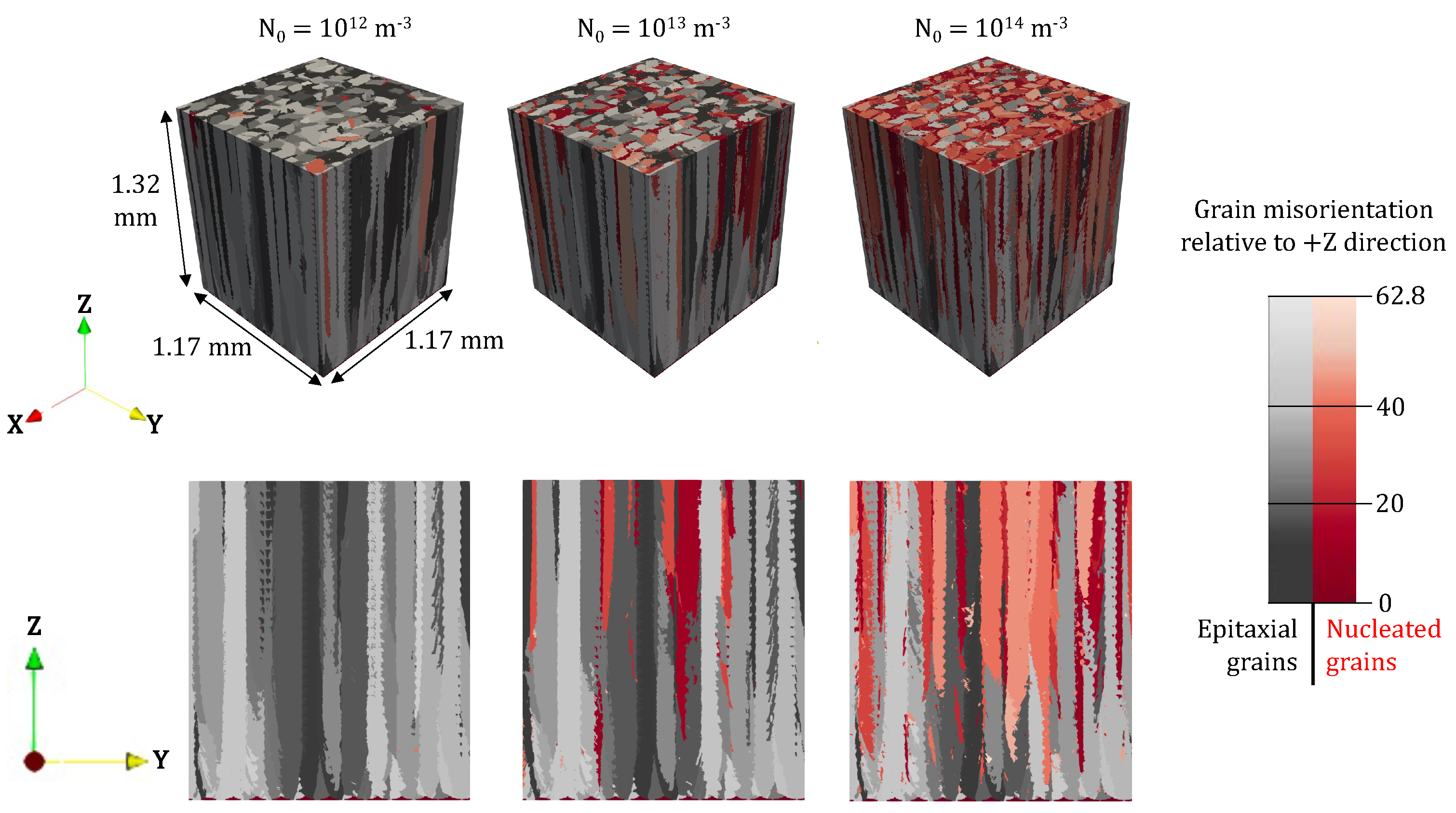
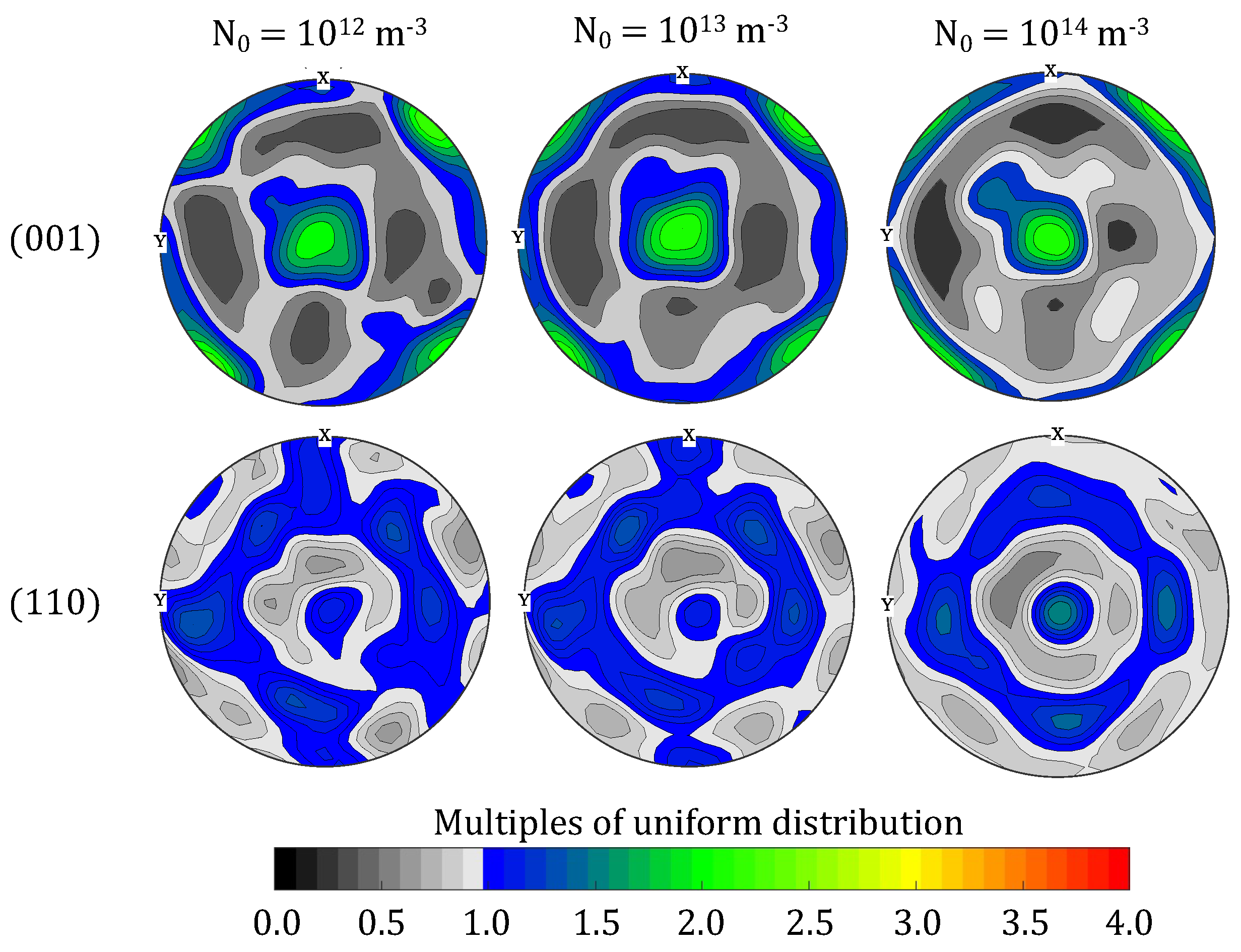
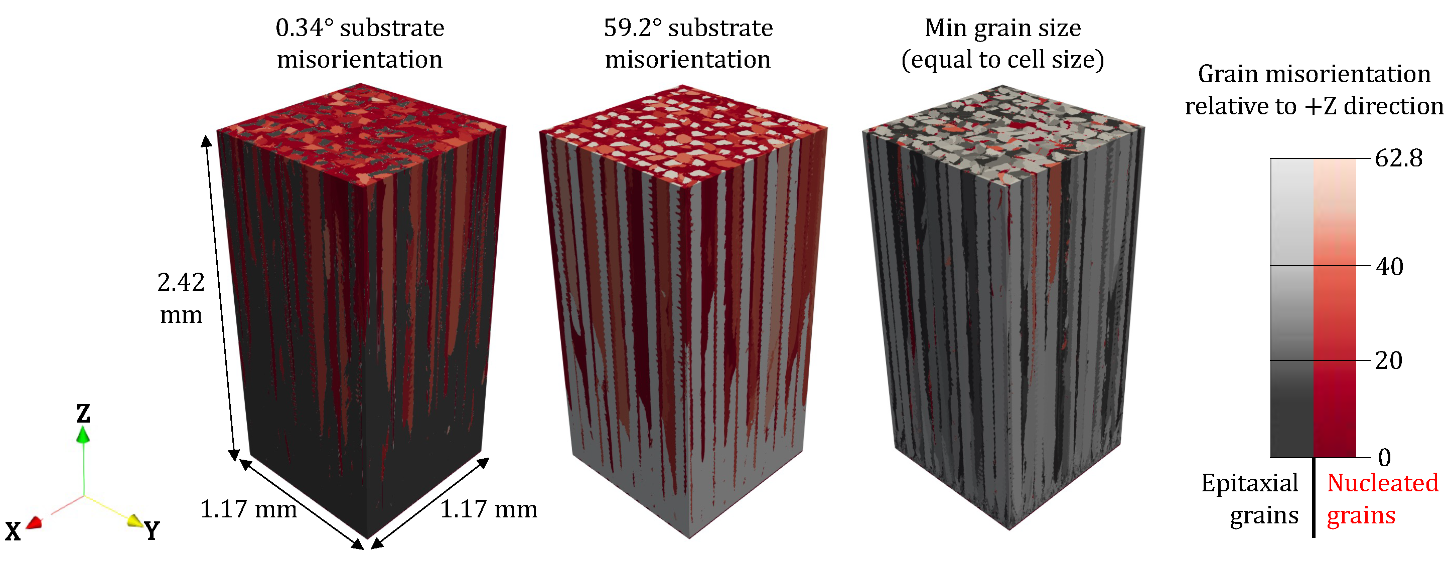
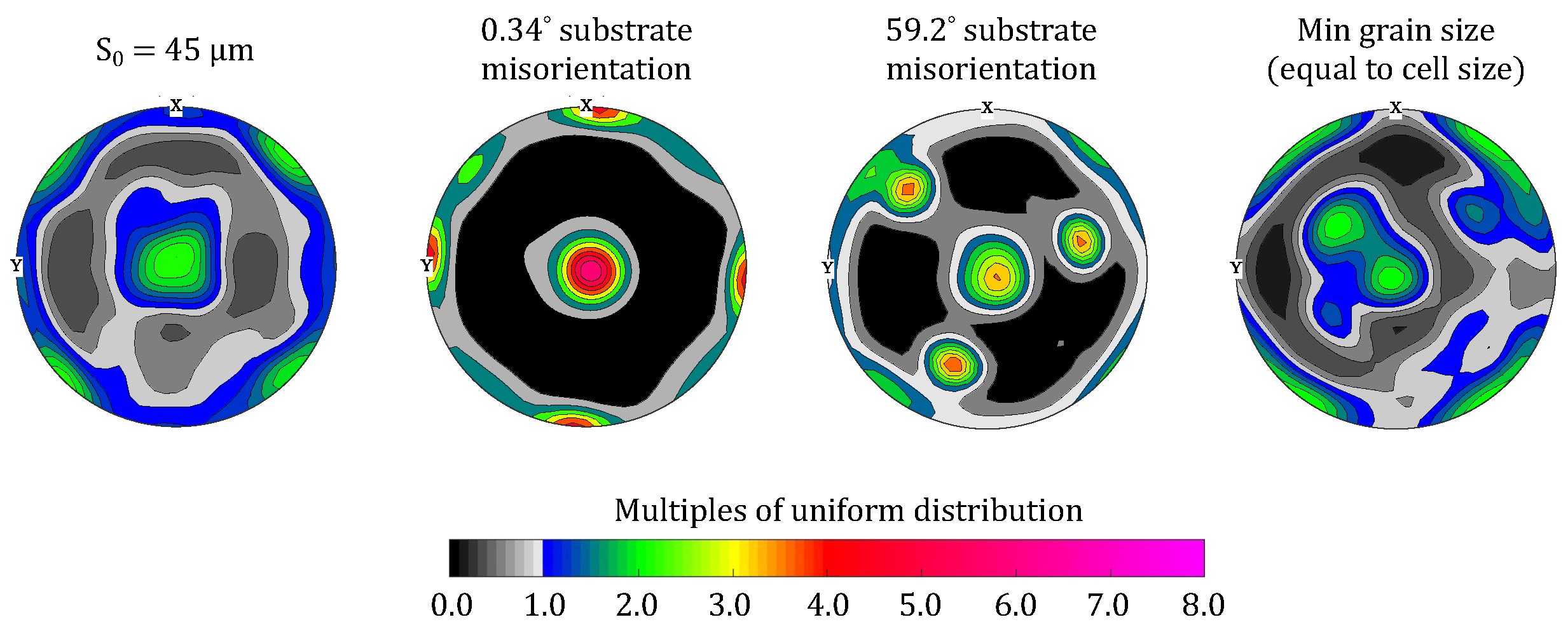
• While $\overline{\varsigma }$ differences due to $N_0$ and $S_0$ were seen throughout the simulated builds (simulations with smaller $S_0$ and larger $N_0$ tending to have smaller grains and reach the steady state more quickly than those with larger $S_0$ and smaller $N_0$), the simulated microstructures were qualitatively similar. The strengths of the 001 and 110 textures, as well as the tall and narrow grain shapes, were similar across all simulations, though it was noted that nucleated grains tended to be more likely than epitaxial grains to have 110 textures.
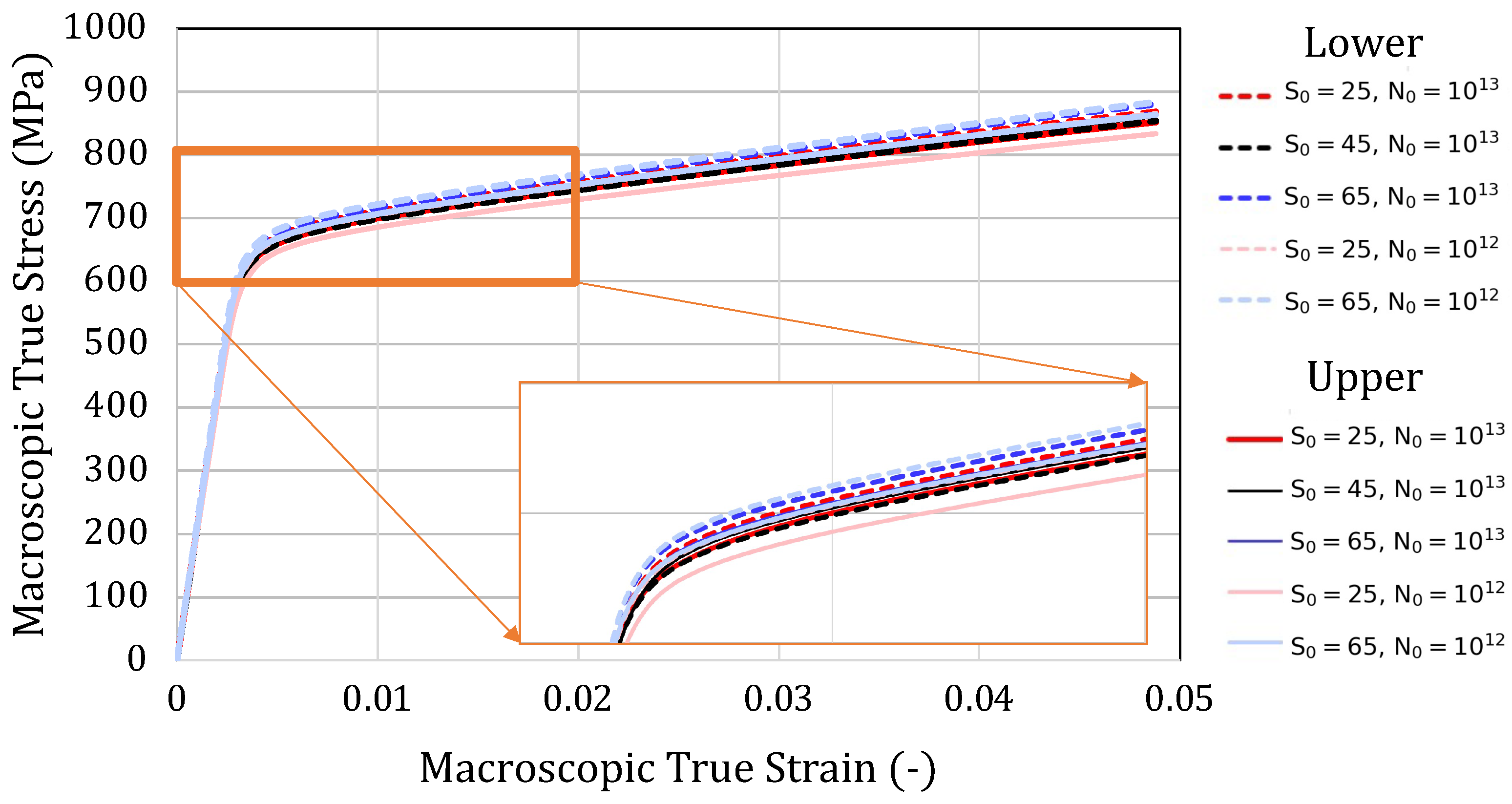
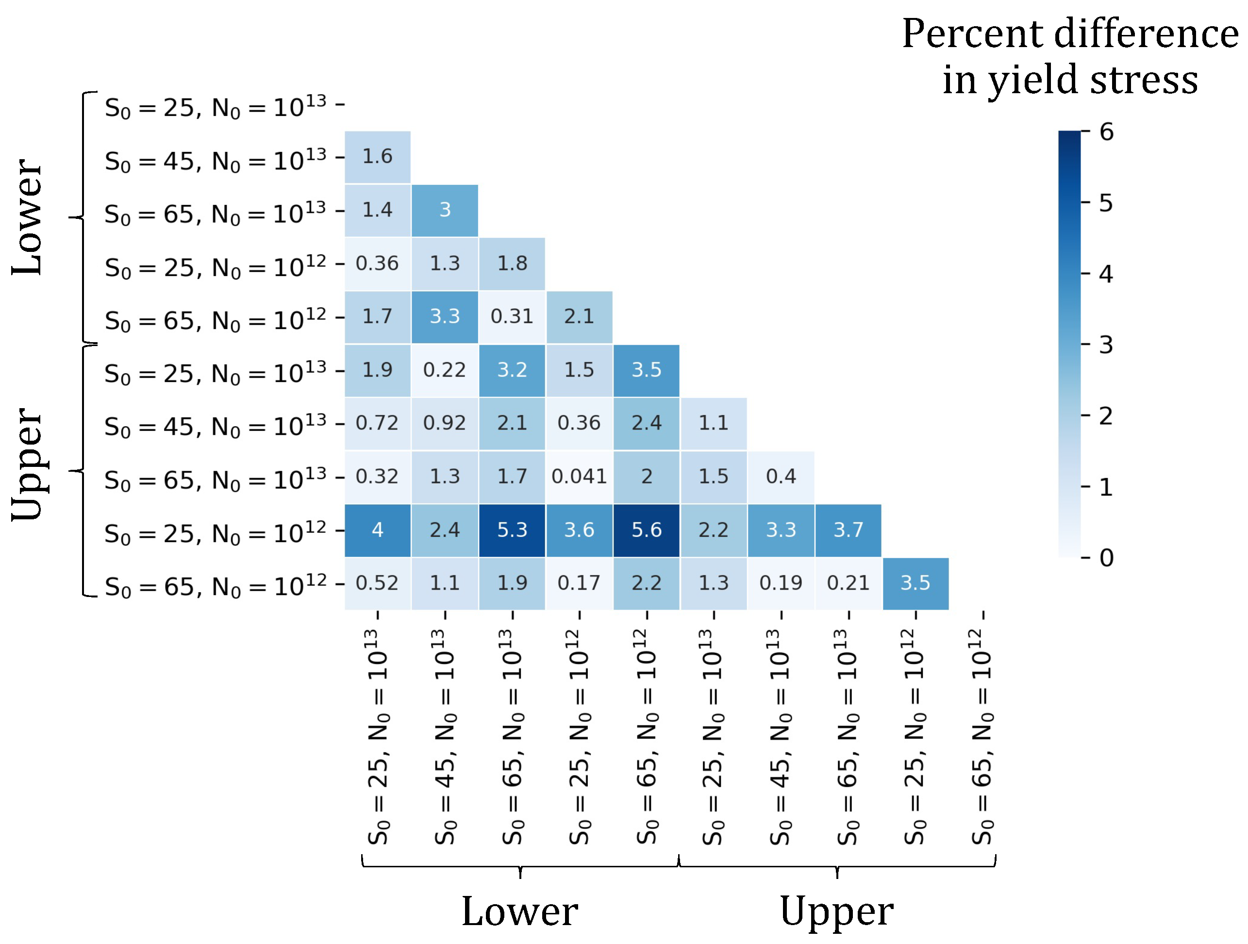
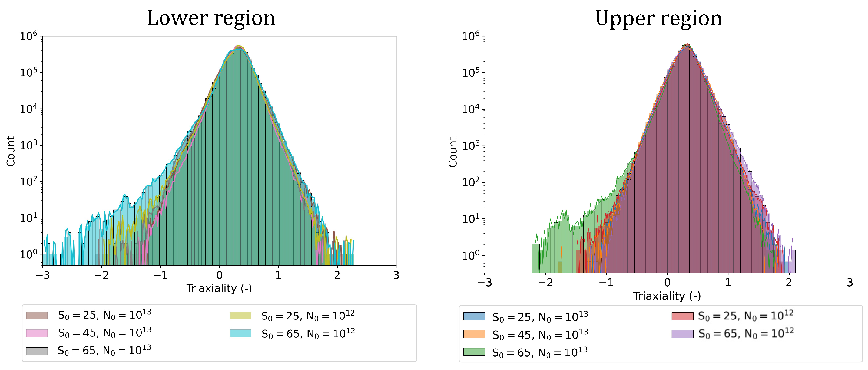
• Using RVEs from different regions of these simulated microstructures as input to ExaConstit calculations, it was found that similar stress–strain behavior and stress triaxiality distributions resulted from RVEs using various permutations of $N_0$ and $S_0$, and yield stress values were within ±6% of each other. Only minor differences were noted in macroscopic mechanical responses between RVEs taken from layers 15 through 39 and RVEs taken from layers 40 through 64, despite differences in $\overline{\varsigma }$ of up to 3x between the RVEs with the smallest and largest grain areas.

We conclude that the initial substrate during simulation of multilayer AM grain growth has a significant effect on grain size development during the first 2 mm of builds for the simulated scan pattern, particularly for small $N_0$ and large $S_0$. In turn, a CA simulation looking to obtain a microstructure representative of a structure far from the baseplate for conditions that favor epitaxial growth should err on the side of smaller $S_0$, particularly when $N_0$ is small. However, reasonable estimations for constitutive mechanical properties can be obtained from simulated grain structures with a range of possible $S_0$ and $N_0$ values. For all $S_0$ and $N_0$ values used, the grain structures and textures were sufficiently similar after 15 simulated layers such that any differences in predicted properties were on the order of the differences due to $S_0$ and $N_0$. This is despite the fact that the microstructures showed non-negligible differences in grain area for different $S_0$, $N_0$, and location in the build, suggesting that the texture and distribution of orientations in space are relatively agnostic to these parameters for the conditions tested. However, we note that when using extremes in $S_0$, such as an extremely small initial grain size or a single grain baseplate, this texture convergence does not readily appear, and that while texture after 15 layers may be relatively insensitive to $S_0$ and $N_0$ for the given material and scan pattern, reasonable input values are still required.

A few caveats apply to the scope of these conclusions. The present study is limited to modeling constitutive property sensitivity to microstructure input, and the sensitivity of microstructure to various uncertain input parameters. In real AM processing, additional physics not accounted for in the present models could complicate the relationships among substrate, nucleation, microstructure as a function of build height, and location-dependent properties. Experimental verification for a given material and scan parameters would be needed to determine to what extent the conclusions drawn regarding microstructure and properties modeling are valid in practice.

In addition to experimental validation of location-specific microstructure, future work using ExaCA includes revising the sparse data assumption from [66], allowing ExaCA analysis using time–temperature history resulting from more complex scan patterns. Generating multiple OpenFOAM input data sets to gauge the relative significance of time–temperature history uncertainty (due to energy absorption, etc) on ExaCA output, relative to the uncertainty in $N_0$ and $S_0$ examined in this study, is also a relevant next step toward consistent prediction of constitutive properties. Future science capability within ExaConstit includes varying the critically resolved shear strength as a function of distance from grain boundaries; a nonuniform resistance to plastic slip would likely yield property predictions that are more sensitive to the varying grain areas observed in the RVEs. Simulation of additional layers within ExaCA to determine the amount of material needed for grain area convergence with small $N_0$ and large $S_0$ may be needed to obtain far from baseplate grain structures, to be fed to an updated ExaConstit that is more sensitive to grain area.

References

- Zhang, W.; Lei, Y.; Meng, W.; Ma, Q.; Yin, X.; Guo, L. Effect of deposition sequence on microstructure and properties of 316L and Inconel 625 bimetallic structure by wire arc additive manufacturing. J. Mater. Eng. Perform. 2021, 30, 8972–8983. [Google Scholar] [CrossRef]
- Calleja-Ochoa, A.; Barrio-Gonzalez, H.; López de Lacalle, N.; Martínez, S.; Albizuri, J.; Lamikiz, A. A new approach in the design of microstructured ultralight components to achieve maximum functional performance. Materials 2021, 14, 1588. [Google Scholar] [CrossRef] [PubMed]
- Collins, P.; Brice, D.; Samimi, P.; Ghamarian, I.; Fraser, H. Microstructural Control of Additively Manufactured Metallic Materials. Annu. Rev. Mater. Res. 2016, 46, 63–91. [Google Scholar] [CrossRef]
- DebRoy, T.; Wei, H.; Zuback, J.; Mukherjee, T.; Elmer, J.; Milewski, J.; Bese, A.M.; Wilson-Heid, A.; De, A.; Zhang, W. Additive manufacturing of metallic components—Process, structure and properties. Prog. Mater. Sci. 2018, 92, 112–224. [Google Scholar] [CrossRef]
- Zhang, X.; Yocom, C.J.; Mao, B.; Liao, Y. Microstructure evolution during selective laser melting of metallic materials: A review. J. Laser Appl. 2019, 31, 031201. [Google Scholar] [CrossRef]
- Oliveira, J.; LaLonde, A.; Ma, J. Processing parameters in laser powder bed fusion metal additive manufacturing. Mater. Des. 2020, 193, 108762. [Google Scholar] [CrossRef]
- Sing, S.; Huang, S.; Goh, G.; Goh, G.; Tey, C.; Tan, J.; Yeong, W. Emerging metallic systems for additive manufacturing: In-situ alloying and multi-metal processing in laser powder bed fusion. Prog. Mater. Sci. 2021, 119, 100795. [Google Scholar] [CrossRef]
- Wan, H.; Zhou, Z.; Li, C.; Chen, G.; Zhang, G. Effect of scanning strategy on grain structure and crystallographic texture of Inconel 718 processed by selective laser melting. J. Mater. Sci. Technol. 2018, 34, 1799–1804. [Google Scholar] [CrossRef]
- Roehling, T.T.; Shi, R.; Khairallah, S.A.; Roehling, J.D.; Guss, G.M.; McKeown, J.T.; Matthews, M.J. Controlling grain nucleation and morphology by laser beam shaping in metal additive manufacturing. Mater. Des. 2020, 195, 109071. [Google Scholar] [CrossRef]
- Lu, Y.; Wu, S.; Gan, Y.; Huang, T.; Yang, C.; Junjie, L.; Lin, J. Study on the microstruture, mechanical property and residual stress of SLM Inconel-718 alloy manufactured by different island scanning strategy. Opt. Laser Technol. 2015, 75, 197–206. [Google Scholar] [CrossRef]
- Raghavan, N.; Simunovic, S.; Dehoff, R.; Plotkowski, A.; Turner, J.; Kirka, M.; Babu, S. Localized melt-scan strategy for site specific control of grain size and primary dendrite arm spacing in electron beam additive manufacturing. Acta Mater. 2017, 140, 375–387. [Google Scholar] [CrossRef]
- Knapp, G.; Raghavan, N.; Plotkowski, A.; DebRoy, T. Experiments and simulations on solidification microstructure for Inconel 718 in powder bed fusion electron beam additive manufacturing. Addit. Manuf. 2019, 25, 511–521. [Google Scholar] [CrossRef]
- Ghayoor, M.; Lee, K.; He, Y.; Chang, C.h.; Paul, B.K.; Pasebani, S. Selective laser melting of 304L stainless steel: Role of volumetric energy density on the microstructure, texture and mechanical properties. Addit. Manuf. 2020, 32, 101011. [Google Scholar] [CrossRef]
- Cheng, M.; Xiao, X.; Luo, G.; Song, L. Integrating control of molten pool technology and solidification texture by adjusting pulse duration in laser additive manufacturing of Inconel 718. Opt. Laser Technol. 2021, 142, 107137. [Google Scholar] [CrossRef]
- Wang, Y.; Chen, X.; Shen, Q.; Su, C.; Zhang, Y.; Jayalakshmi, S.; Singh, R.A. Effect of magnetic field on the microstructure and mechanical properties of inconel 625 superalloy fabricated by wire arc additive manufacturing. J. Manuf. Process. 2021, 64, 10–19. [Google Scholar] [CrossRef]
- Todaro, C.; Easton, M.; Qiu, D.; Zhang, D.; Bermingham, M.; Lui, E.; Brandt, M.; StJohn, D.; Qian, M. Grain structure control during metal 3D printing by high-intensity ultrasound. Nat. Commun. 2020, 11, 142. [Google Scholar] [CrossRef]
- Ma, Q.; Chen, H.; Ren, N.; Zhang, Y.; Hu, L.; Meng, W.; Yin, X. Effects of ultrasonic vibration on microstructure, mechanical properties, and fracture mode of Inconel 625 parts fabricated by cold metal transfer arc additive manufacturing. J. Mater. Eng. Perform. 2021, 30, 6808–6820. [Google Scholar] [CrossRef]
- Pérez-Ruiz, J.D.; Martin, F.; Martínez, S.; Lamikiz, A.; Urbaikain, G.; López de Lacalle, L.N. Stiffening near-net-shape functional parts of Inconel 718 LPBF considering material anisotropy and subsequent machining issues. Mech. Syst. Process. 2022, 168, 108675. [Google Scholar] [CrossRef]
- Köhen, P.; Ewald, S.; Schleifenbaum, J.H.; Belyakov, A.; Haase, C. Controlling microstructure and mechanical properties of additively manufactured high-strength steels by tailored solidification. Addit. Manuf. 2020, 35, 101389. [Google Scholar]
- Bermingham, M.; StJohn, D.; Krynen, J.; Tedman-Jones, S.; Dargusch, M. Promoting the columnar to equiaxed transtion and grain refinement of titanium alloys during additive manufacturing. Acta Mater. 2019, 168, 261–274. [Google Scholar] [CrossRef]
- Tang, Y.T.; Panwisawas, C.; Ghoussoub, J.N.; Gong, Y.; Clark, J.W.; Nemeth, A.A.; McCartney, D.G.; Reed, R.C. Alloys-by-design: Application to new superalloys for additive manufacturing. Acta Mater. 2021, 202, 417–436. [Google Scholar] [CrossRef]
- Turner, J.A.; Belak, J.; Barton, N.; Bement, M.; Carlson, N.; Carson, R.; DeWitt, S.; Fattebert, J.L.; Hodge, N.; Jibben, Z.; et al. ExaAM: Metal additive manufacturing simulation at the fidelity of the microstructure. Int. J. High Perform. Comput. Appl. 2022, 36, 13–39. [Google Scholar] [CrossRef]
- OpenFOAM. 2021. Available online: https://github.com/OpenFOAM (accessed on 7 February 2022).
- Coleman, J.; Plotkowski, A.; Stump, B.; Raghavan, N.; Sabau, A.; Krane, M.; Heigel, J.; Ricker, R.; Levine, L.; Babu, S. Sensitivity of Thermal Predictions to Uncertain Surface Tension Data in Laser Additive Manufacturing. J. Heat Transf. 2020, 142, 122201. [Google Scholar] [CrossRef]
- Rolchigo, M.; Reeve, S.; Stump, J. ExaCA. 2021. Available online: https://github.com/LLNL/ExaCA (accessed on 7 February 2022).
- Carson, R.A.; Wopschall, S.R.; Bramwell, J.A. ExaConstit. 2019. Available online: https://www.osti.gov/doecode/biblio/31691 (accessed on 7 February 2022).
- Basak, A.; Das, S. Epitaxy and Microstructure Evolution in Metal Additive Manufacturing. Annu. Rev. Mater. Res. 2016, 46, 125–149. [Google Scholar] [CrossRef]
- Wang, D.; Song, C.; Yang, Y.; Bai, Y. Investigation of crystal growth mechanism during selectiv laser melting and mechanical property characterization of 316L stainless steel parts. Mater. Des. 2016, 100, 291–299. [Google Scholar] [CrossRef]
- Bai, L.; Le, G.; Liu, X.; Li, J.; Xia, S.; Li, X. Grain morphologies and microstructures of laser melting depositied V-5Cr-5Ti alloys. J. Alloys Compd. 2018, 745, 716–724. [Google Scholar] [CrossRef]
- Wei, H.; Mazumder, J.; DebRoy, T. Evolution of solidification texture during additive manufacturing. Sci. Rep. Nat. 2015, 5, 16446. [Google Scholar] [CrossRef] [Green Version]
- Pham, M.S.; Dovgyy, B.; Hooper, P.A.; Gourlay, C.M.; Piglione, A. The role of side-branching in microstructure development in laser powder-bed fusion. Nat. Commun. 2020, 11, 749. [Google Scholar] [CrossRef]
- Kok, Y.; Tan, X.; Wang, P.; Nai, M.; Loh, N.; Liu, E.; Tor, S. Anisotropy and heterogeneity of microstructure and mechanical properties in metal additive manufacturing: A critical review. Mater. Des. 2018, 139, 565–586. [Google Scholar] [CrossRef]
- Shamsaei, N.; Yadollahi, A.; Bian, L.; Thompson, S.M. An overview of Direct Laser Deposition for additive manufacturing; Part II: Mechanical behavior, process parameter optimization and control. Addit. Manuf. 2015, 8, 12–35. [Google Scholar] [CrossRef]
- Tian, Z.; Zhang, C.; Wang, D.; Liu, W.; Fang, X.; Wellman, D.; Zhao, Y.; Tian, Y. A review on laser powder bed fusion of Inconel 625 nickel-based alloy. Appl. Sci. 2020, 10, 81. [Google Scholar] [CrossRef] [Green Version]
- Li, J.; Zhou, X.; Brochu, M.; Provatas, N.; Zhao, Y.F. Solidification microstructure simulation of Ti-6Al-4V in metal additive manufacturing: A review. Addit. Manuf. 2020, 31, 100989. [Google Scholar] [CrossRef]
- Gatsos, T.; Elsayed, K.A.; Zhai, Y.; Lados, D.A. Review on Computational Modeling of Process-Microstructure-Property Relatonships in Metal Additive Manufacturing. JOM 2020, 72, 403–419. [Google Scholar] [CrossRef]
- Rappaz, M.; Gandin, C.A. Probabilistic modeling of microstructure formation in solidification processes. Acta Metall. Et Mater. 1993, 41, 345–360. [Google Scholar] [CrossRef]
- Gandin, C.A.; Rappaz, M. A coupled finite-element cellular-automaton model for the prediction of dendritic grain structures in solidification processes. Acta Metall. Mater. 1994, 42, 2233–2246. [Google Scholar] [CrossRef]
- Gandin, C.A.; Rappaz, M. A 3D cellular automaton algorithm for the prediction of dendritic grain growth. Acta Mater. 1997, 45, 2187–2195. [Google Scholar] [CrossRef]
- Zinoviev, A.; Zinovieva, O.; Ploshikhin, V.; Romanova, V.; Balokhonov, R. Evolution of grain structure during laser additive manufacturing. Simulation by a cellular automata method. Mater. Des. 2016, 106, 321–329. [Google Scholar] [CrossRef]
- Rai, A.; Markl, M.; Korner, C. A coupled Cellular Automaton-Lattice Boltzmann model for grain structure simulation during additive manufacturing. Comput. Mater. Sci. 2016, 124, 37–48. [Google Scholar] [CrossRef]
- Zinovieva, O.; Zinoviev, A.; Ploshikhin, V. Three-dimensional modeling of the microstructure evolution during metal additive manufacturing. Comput. Mater. Sci. 2018, 141, 207–220. [Google Scholar] [CrossRef]
- Akram, J.; Chalavadi, P.; Pal, D.; Stucker, B. Understanding grain evolution in additive manufacturing through modeling. Addit. Manuf. 2018, 21, 255–268. [Google Scholar] [CrossRef]
- Koepf, J.A.; Goterbarm, M.R.; Markl, M.; Körner, C. 3D multi-layer grain structure simulation of powder bed fusion additive manufacturing. Acta Mater. 2018, 152, 119–126. [Google Scholar] [CrossRef]
- Liu, D.R.; Wang, S.; Yan, W. Grain structure evolution in transition-mode melting in direct energy deposition. Mater. Des. 2020, 194, 108919. [Google Scholar] [CrossRef]
- Wang, Z.; Lin, X.; Kang, N.; Hu, Y.; Chen, J.; Huang, W. Strength-ductility synergy of selective laser melted Al-Mg-Sc-Zr alloy with a heterogenous grain structure. Addit. Manuf. 2020, 34, 101260. [Google Scholar]
- Yang, J.; Yu, H.; Yang, H.; Li, F.; Wang, Z.; Zeng, X. Prediction of microstructure in selective laser melted Ti-6Al-4V alloy by cellular automaton. J. Alloys Compd. 2018, 748, 281–290. [Google Scholar] [CrossRef]
- Li, M.; Li, J.M.; Zheng, Q.; Wang, G.; Zhang, M.X. Effect of solutes on grain refinement of as-cast Fe-4Si alloy. Metall. Mater. Trans. A 2018, 49A, 2235–2247. [Google Scholar] [CrossRef]
- Lian, Y.; Gan, Z.; Yu, C.; Kats, D.; Liu, W.K.; Wagner, G.J. A cellular automaton finite volume method for microstructure evolution during additive manufacturing. Mater. Des. 2019, 169, 107672. [Google Scholar] [CrossRef]
- Mohebbi, M.S.; Ploshikhin, V. Implementation of nucleation in cellular automaton simulation of microstructural evolution during additive manufacturing of Al alloys. Addit. Manuf. 2020, 36, 101726. [Google Scholar] [CrossRef]
- Dezfoli, A.R.A.; Lo, Y.L.; Raza, M.M. Prediction of epitaxial grain growth in single-track laser melting of IN718 using integrated finite element and cellular automaton approach. Materials 2021, 14, 5202. [Google Scholar] [CrossRef]
- Xiong, F.; Huang, C.; Kafka, O.L.; Lian, Y.; Yan, W.; Chen, M.; Fang, D. Grain growth prediction in selective electron beam melting of Ti-6Al-4V with a cellular automaton method. Mater. Des. 2021, 199, 109410. [Google Scholar] [CrossRef]
- Anderson, T.D.; DuPont, J.N.; DebRoy, T. Origin of stray grain formation in single-crystal superalloy weld pools from heat transfer and fluid flow modeling. Acta Mater. 2010, 58, 1441–1454. [Google Scholar] [CrossRef]
- Wang, T.; Zhu, Y.; Zhang, S.; Tang, H.; Wang, H. Grain morphology evolution during behavior of titanium alloy components during laser melting deposition additive manufacturing. J. Alloys Compd. 2015, 632, 505–513. [Google Scholar] [CrossRef]
- Sabau, A.S.; Yuan, L.; Raghavan, N.; Bement, M.; Simunovic, S.; Turner, J.A.; Gupta, V.K. Fluid dynamics effects on microstructure predition in single-laser tracks for additive manuacturing of IN625. Metall. Trans. B 2020, 51, 1263–1281. [Google Scholar] [CrossRef] [Green Version]
- Liu, Y.; Liu, Z.; Jiang, Y.; Wang, G.; Yang, Y.; Zhang, L. Gradient in microstructure and mechanical property of selective laser melted AlSi10Mg. J. Alloys Compd. 2018, 735, 1414–1421. [Google Scholar] [CrossRef]
- Li, Z.; Chen, J.; Sui, S.; Zhong, C.; Lu, X.; Lin, X. The microstructure evolution and tensile properties of Inconel 718 fabricated by high-deposition-rate laser directed energy deposition. Addit. Manuf. 2020, 31, 100941. [Google Scholar] [CrossRef]
- Dinda, G.; Dasgupta, A.; Mazumder, J. Evolution of microstructure in laser depositied Al-11.28%Si alloy. Surf. Coat. Technol. 2012, 206, 2152–2160. [Google Scholar] [CrossRef]
- Al-Bermani, S.S.; Blackmore, M.L.; Zhang, W.; Todd, I. The Origin of Microstructural Diversity, Texture, and Mechanical Properties in Electron Beam Melted Ti-6Al-4V. Metall. Mater. Trans. A-Phys. Metall. Mater. Sci. 2010, 41, 3422–3434. [Google Scholar] [CrossRef]
- Kergassner, A.; Koepf, J.A.; Markl, M.; Korner, C.; Mergheim, J.; Steinmann, P. A novel approach to predict the process-induced mechanical behavior of additively manufactured materials. J. Mater. Eng. Perform. 2021, 30, 5235–5246. [Google Scholar] [CrossRef]
- Lim, H.; Abdeljawad, F.; Owen, S.J.; Hanks, B.W.; Foulk, J.W.; Battaile, C.C. Incorporating physically-based microstructures in materials modeling: Bridging phase field and crystal plasticity frameworks. Model. Simul. Mater. Sci. Eng. 2016, 24, 045016. [Google Scholar] [CrossRef]
- Kergassner, A.; Mergheim, J.; Steinmann, P. Modeling of additively manufactured materials using gradient-enhances crystal plasticity. Comput. Math. Appl. 2019, 78, 2338–2350. [Google Scholar] [CrossRef]
- Romanova, V.; Balokhonov, R.; Zinovieva, O.; Emelianova, E.; Dymnich, E.; Pisarev, M.; Zinoviev, A. Micromechanical simulations of additive manufactured aluminum alloys. Comput. Struct. 2021, 244, 106412. [Google Scholar] [CrossRef]
- Yan, W.; Lian, Y.; Yu, C.; Kafka, O.L.; Liu, Z.; Liu, W.K.; Wagner, G.J. An integrated process-structure-property modeling framework for additive manufacturing. Comput. Methods Appl. Mech. Eng. 2018, 339, 184–204. [Google Scholar] [CrossRef]
- Heo, T.W.; Khairallah, S.A.; Shi, R.; Berry, J.; Perron, A.; Calta, N.P.; Martin, A.A.; Barton, N.A.; Roehling, J.; Roehling, T.; et al. A mesoscopic digital twin that bridges length and time scales for control of additively manufactured metal microstructures. J. Phys. Mater. 2021, 4, 034012. [Google Scholar] [CrossRef]
- Rolchigo, M.; Stump, B.; Belak, J.; Plotkowski, A. Sparse thermal data for cellular automata modeling of grain structure in additive manufacturing. Model. Simul. Mater. Sci. Eng. 2020, 28, 065003. [Google Scholar] [CrossRef]
- Bragard, J.; Karma, A.; Lee, Y. Linking Phase-Field and Atomistic Simulations to Model Dendritic Solidification in Highly Undercooled Melts. Interface Sci. 2002, 10, 121–126. [Google Scholar] [CrossRef]
- Teferra, K.; Rowenhorst, D.J. Optimizing the cellular automata finite element model for additive manufacturing to simulate large microstructures. Acta Mater. 2021, 213, 116930. [Google Scholar] [CrossRef]
- MacKenzie, J. Second paper on statistics associated with the random disorientation of cubes. Biometrika 1958, 45, 229–240. [Google Scholar] [CrossRef]
- Barton, N.R.; Carson, R.A.; Wopschall, S.R. ECMech. 2018. Available online: https://www.osti.gov/doecode/biblio/28720 (accessed on 7 February 2022).
- MFEM: Modular Finite Element Methods Library. Available online: https://www.osti.gov/doecode/biblio/35738 (accessed on 7 February 2022).
- Marin, E.; Dawson, P. On modelling the elasto-viscoplastic response of metals using polycrystal plasticity. Comput. Methods Appl. Mech. Eng. 1998, 165, 1–21. [Google Scholar] [CrossRef]
- Moore, J.A.; Barton, N.R.; Florando, J.; Mulay, R.; Kumar, M. Crystal plasticity modeling of β phase deformation in Ti-6Al-4V. Model. Simul. Mater. Sci. Eng. 2017, 25, 075007. [Google Scholar] [CrossRef]
- Wang, Z.; Stoica, A.D.; Ma, D.; Beese, A.M. Diffraction and single-crystal elastic constants of Inconel 625 at room and elevated temperatures determined by neutron diffraction. Mater. Sci. Eng. A 2016, 674, 406–412. [Google Scholar] [CrossRef] [Green Version]
- Groeber, M.; Schwalbach, E.; Donegan, S.; Uchic, M.; Chapman, M.; Shade, P.; Musinski, W.; Miller, J.; Turner, T.; Sparkman, D.; et al. AFRL AM Modeling Challenge Series: Challenge 3 Data Package. 2018. Available online: https://acdc.alcf.anl.gov/mdf/detail/groebermichael_afrl_am_package_v1.1/ (accessed on 7 February 2022).
- Barlat, F.; Aretz, H.; Yoon, J.; Karabin, M.; Brem, J.; Dick, R. Linear transfomation-based anisotropic yield functions. Int. J. Plast. 2005, 21, 1009–1039. [Google Scholar] [CrossRef]
- Barton, N.R.; Knap, J.; Arsenlis, A.; Becker, R.; Hornung, R.D.; Jefferson, D.R. Embedded polycrystal plasticity and adaptive sampling. Int. J. Plast. 2008, 24, 242–266. [Google Scholar] [CrossRef]
- Knap, J.; Barton, N.R.; Hornung, R.D.; Arsenlis, A.; Becker, R.; Jefferson, D.R. Adaptive sampling in hierarchical simulation. Int. J. Numer. Methods Eng. 2008, 76, 572–600. [Google Scholar] [CrossRef]
- Van Houtte, P.; Yerra, S.K.; Van Bael, A. The Facet method: A hierarchical multilevel modelling scheme for anisotropic convex plastic potentials. Int. J. Plast. 2009, 25, 332–360. [Google Scholar] [CrossRef]
- Segurado, J.; Lebensohn, R.A.; LLorca, J.; Tomé, C.N. Multiscale modeling of plasticity based on embedding the viscoplastic self-consistent formulation in implicit finite elements. Int. J. Plast. 2012, 28, 124–140. [Google Scholar] [CrossRef]
- Gawad, J.; Banabic, D.; Van Bael, A.; Comsa, D.S.; Gologanu, M.; Eyckens, P.; Van Houtte, P.; Roose, D. An evolving plane stress yield criterion based on crystal plasticity virtual experiments. Int. J. Plast. 2015, 75, 141–169. [Google Scholar] [CrossRef]
- Zhang, H.; Diehl, M.; Roters, F.; Raabe, D. A virtual laboratory using high resolution crystal plasticity simulations to determine the initial yield surface for sheet metal forming operations. Int. J. Plast. 2016, 80, 111–138. [Google Scholar] [CrossRef]
- Chu, C.C.; Needleman, A. Void Nucleation Effects in Biaxially Stretched Sheets. J. Eng. Mater. Technol. 1980, 102, 249–256. [Google Scholar] [CrossRef]