
Parameter Identification of the Yoshida-Uemori Hardening Model for Remanufacturing

Abstract
:1. Introduction
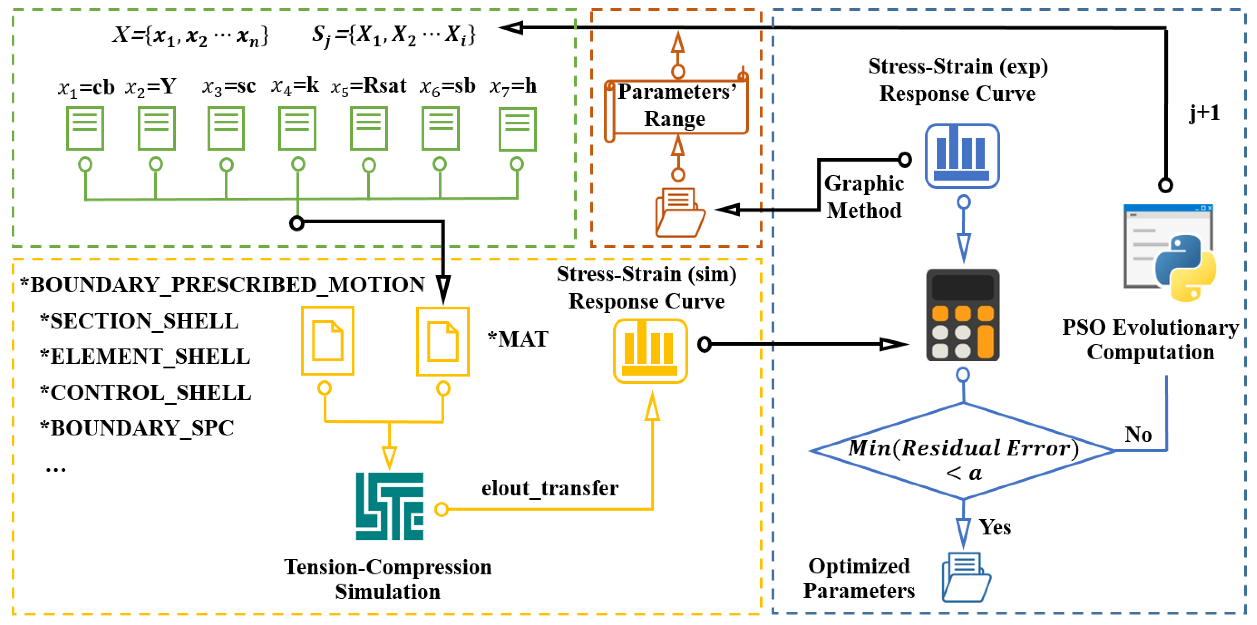
2. Methodology
- (1)
- Set the parameters’ range and initialize the particle swarm. As with the stress-strain response curve of the tensile-compression experiment, the approximate parameters group for the Y-U hardening model is calculated analytically. Based on these calculations, the parameter range should be narrowed, which will potentially reduce the PSO section iterations. The particle swarm including i groups of parameters should be randomly selected.
- (2)
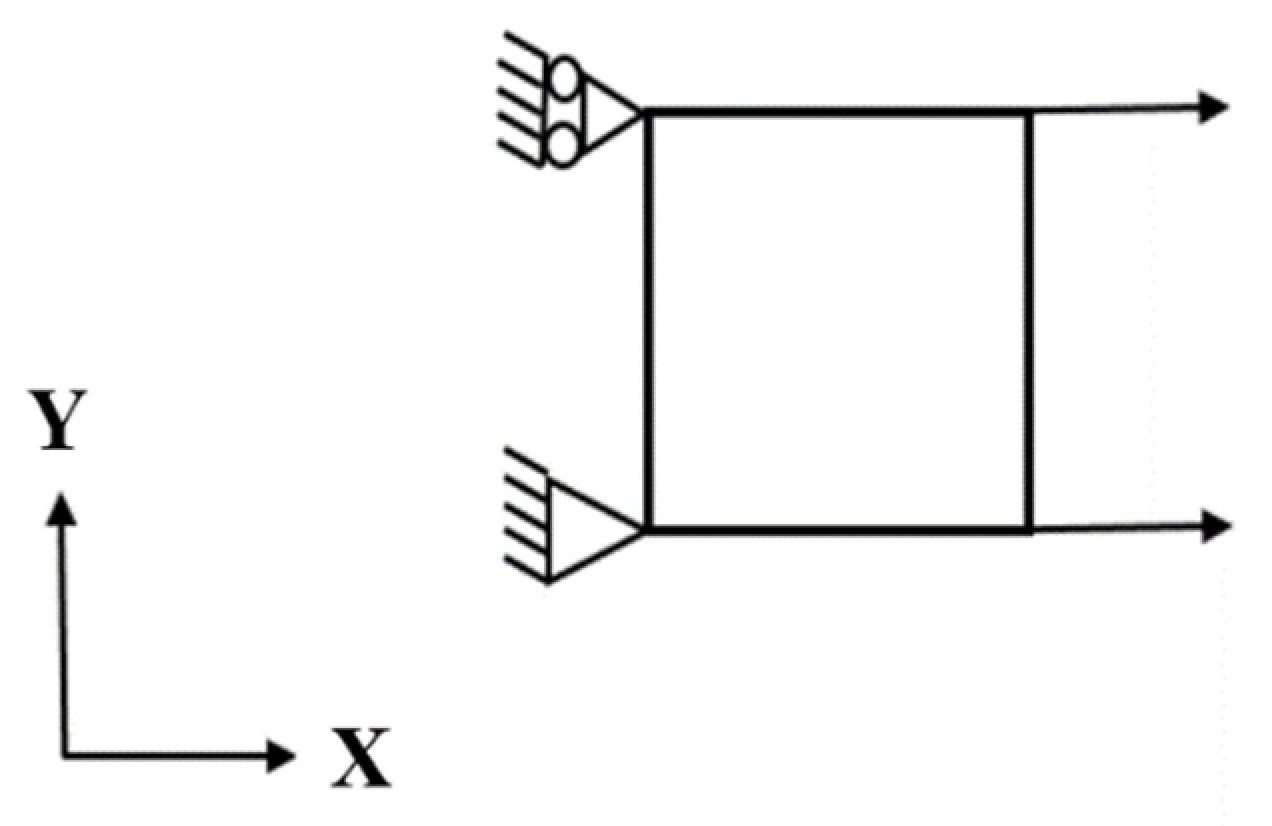
- Predict the response curve by simulation. The simulation uses a four-node shell element, with an element size of 1 × 1 mm. The cyclic displacement is loaded in the X-axis direction (the boundary conditions are shown in Figure 2). Import the i groups of parameters for the jth iteration to obtain the predicted response curves.
- (3)
- Calculate the residual error as fitness value. Determine whether the residual error between the experiment results and the simulation results satisfies the accuracy requirement. If the accuracy is satisfied, skip to step 5. Otherwise, continue to step 4.
- (4)
- Proceed to the next iteration. Take the i groups of parameters with residual errors as fitting values into the particle swarm iteration, generate the new particle swarm and jump to step 2 for the j + 1st iteration.
- (5)
- Terminate the iteration with an optimal particle. Obtain optimized parameters group with satisfied residual error for the Y-U hardening model.
2.1. Yoshida-Uemori Hardening Model
2.2. Graphical Section
- (1)
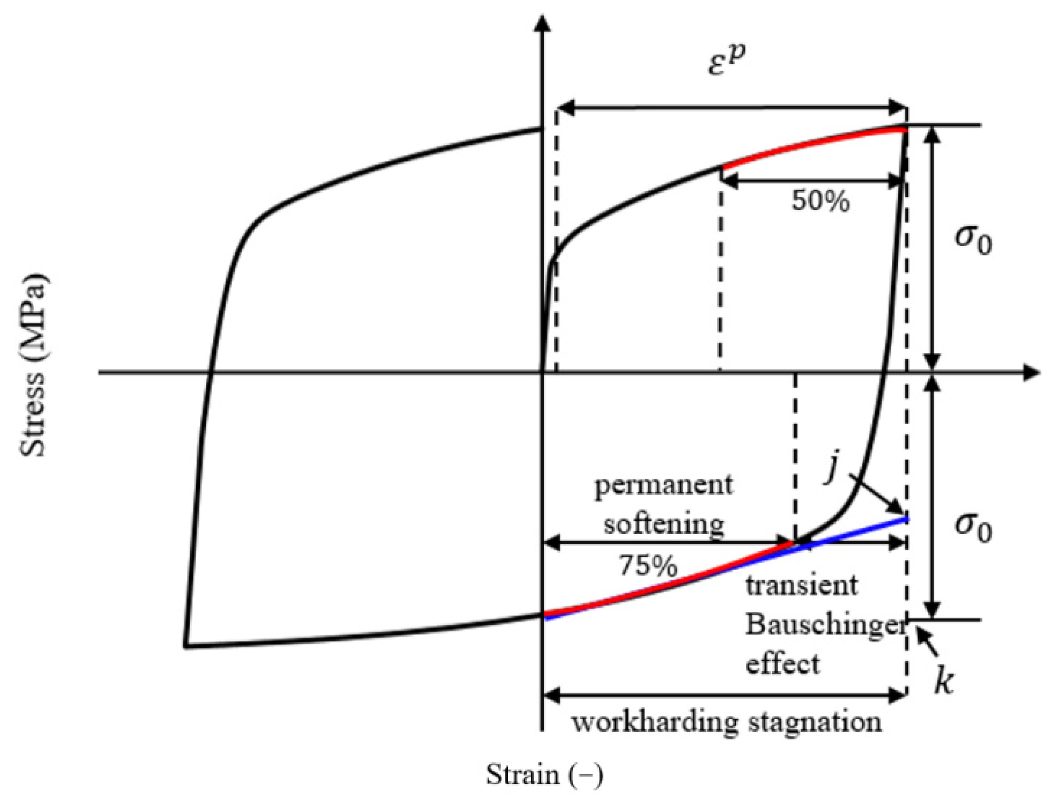
- Determine the parameter Y. Fit the data points of the elastic deformation stage to a straight line. Offset 0.2% to intersect with the experiment stress-strain curve and obtain the parameter Y value.
- (2)
- Determine the parameter cb and k. The voce hardening model is used to describe the tensile flow stress. Fit 50% of the curve with Equation (4) and get the values of cb, k and sb + Rsat.
- (3)
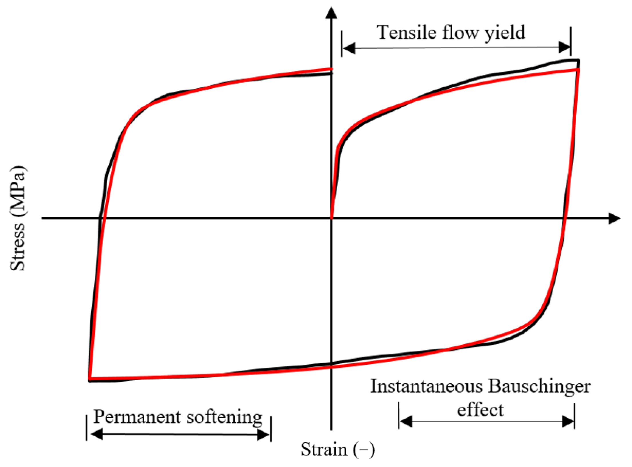
- Determine the parameters sb and Rsat. While uniaxial compression reaches the plastic strain, point (k) represents the fixed isotropic boundary. Point (j) is the intersection of the permanent softening fitting line and the maximum tensile strain. Equation (5) describes the relationship between point (k) and point (j). The parameter sb can be calculated with the known parameter k to achieve the parameter Rsat.
- (4)
- Determine parameters C and h. C is involved in the stress-strain relationship as follows:
2.3. PSO Section
2.4. PSO Variations
3. Case Study
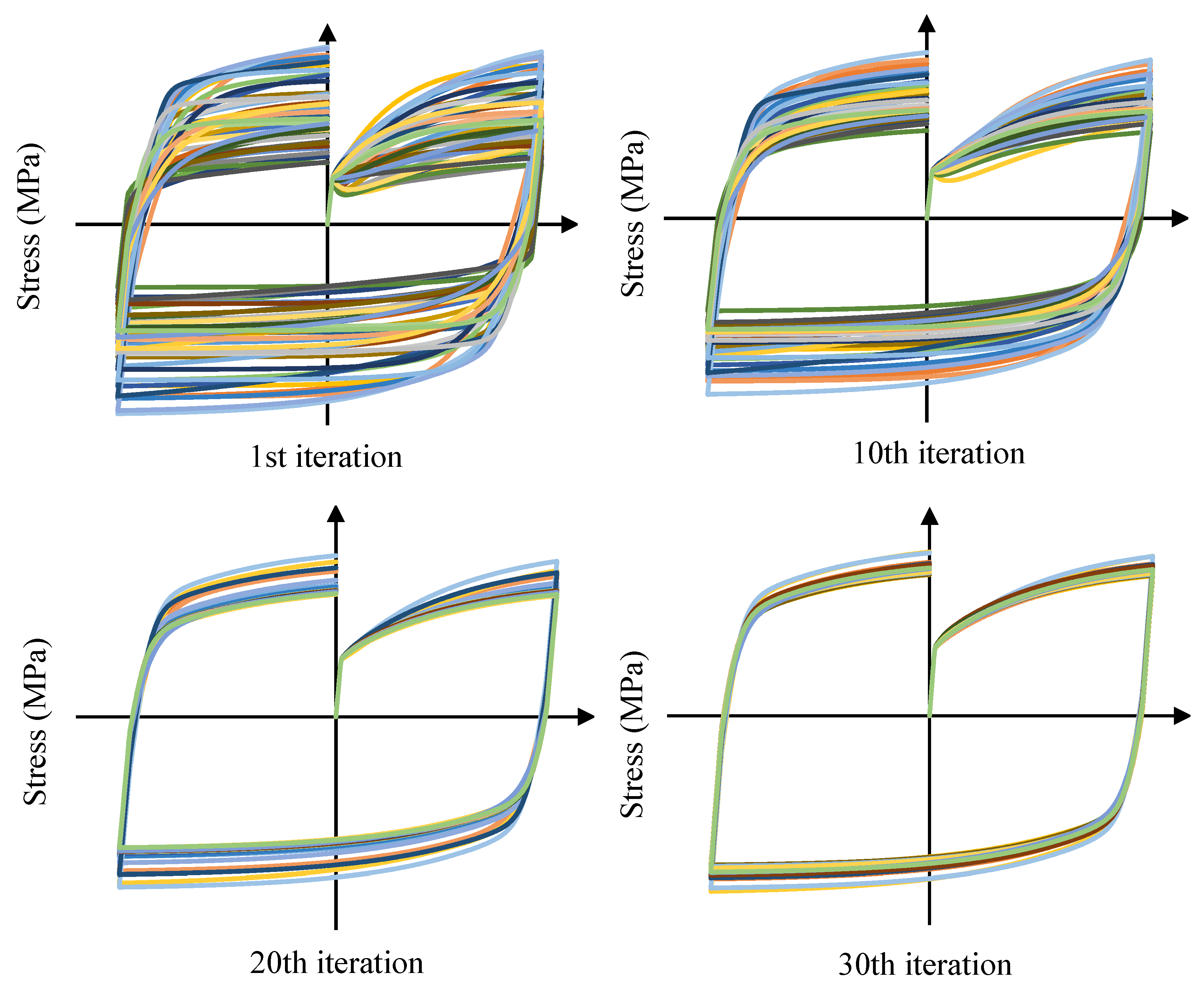
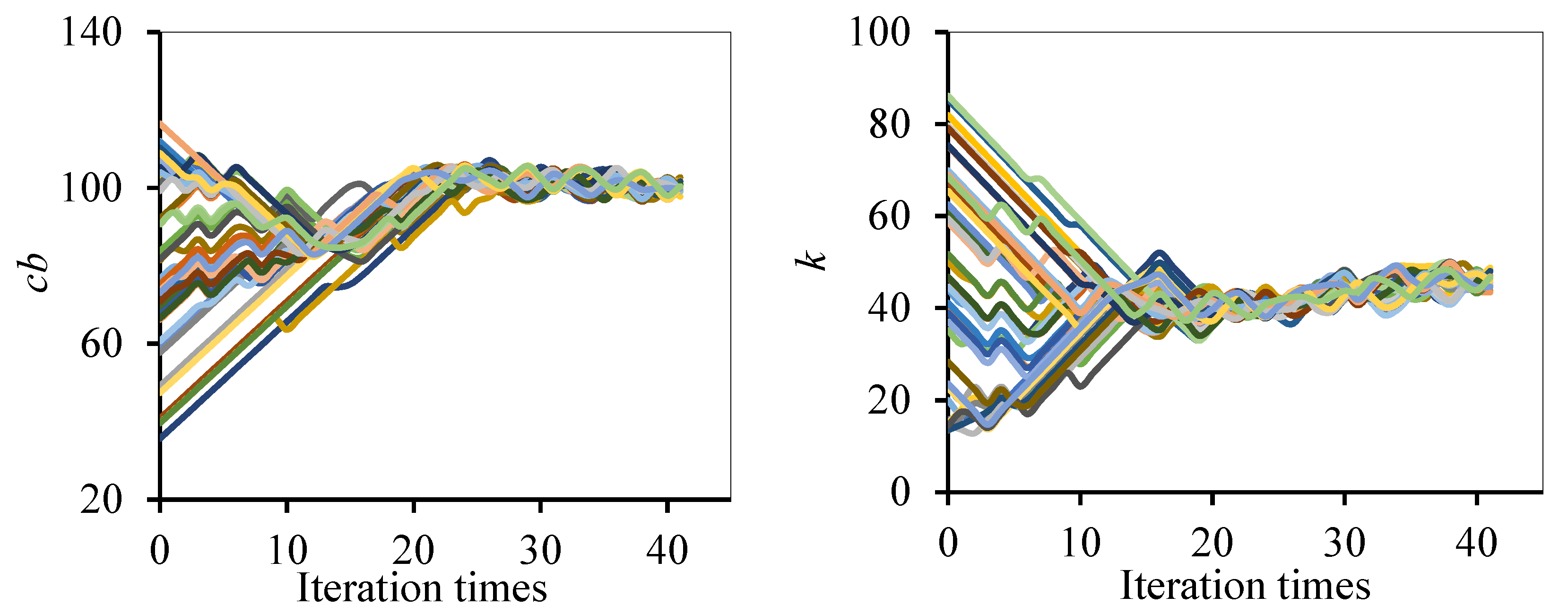
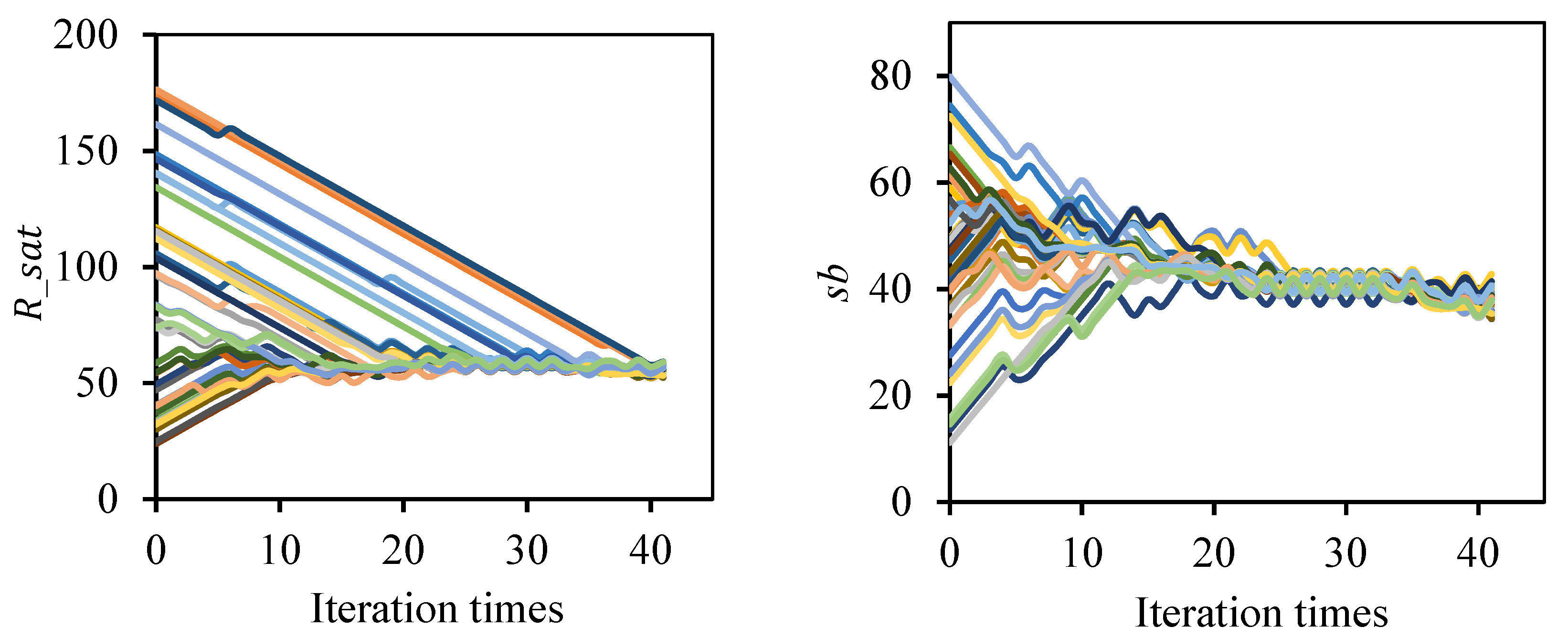
3.1. Optimization Process
3.2. Results
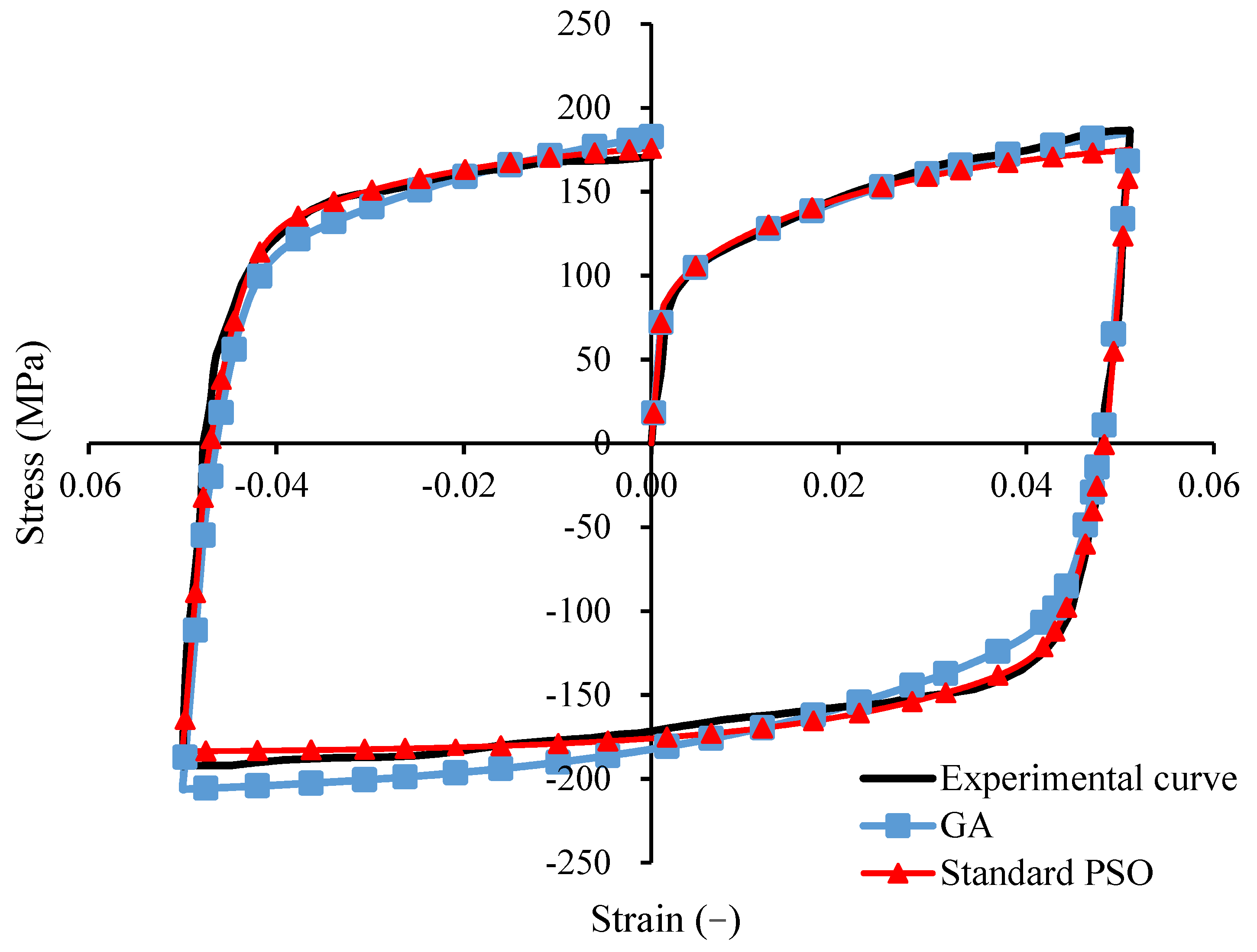
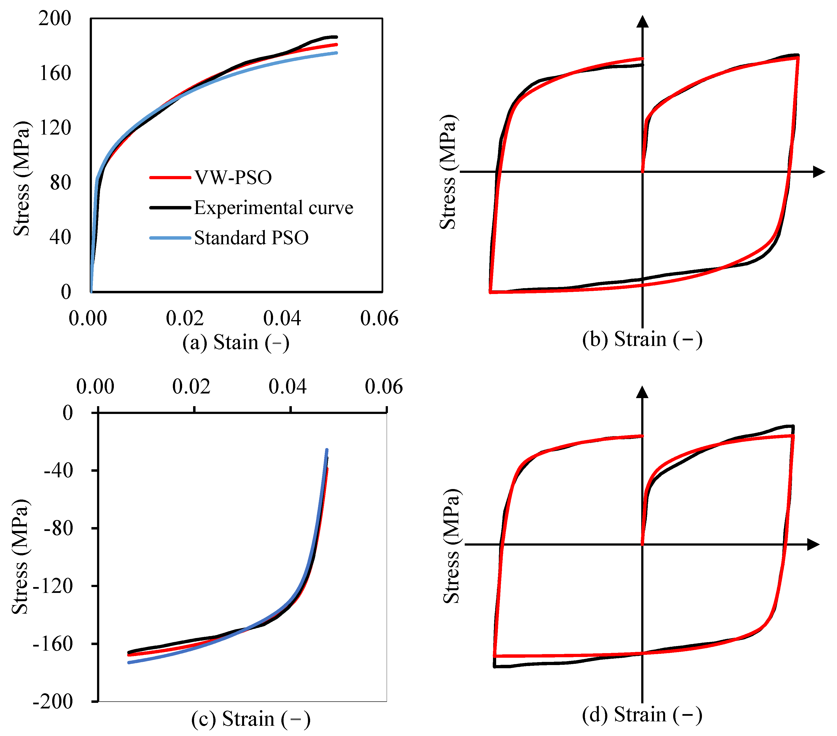
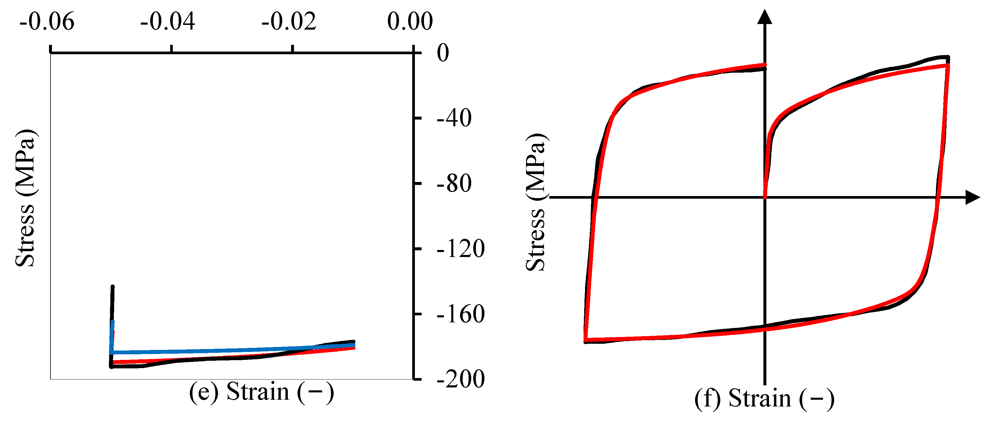
3.3. Discussion
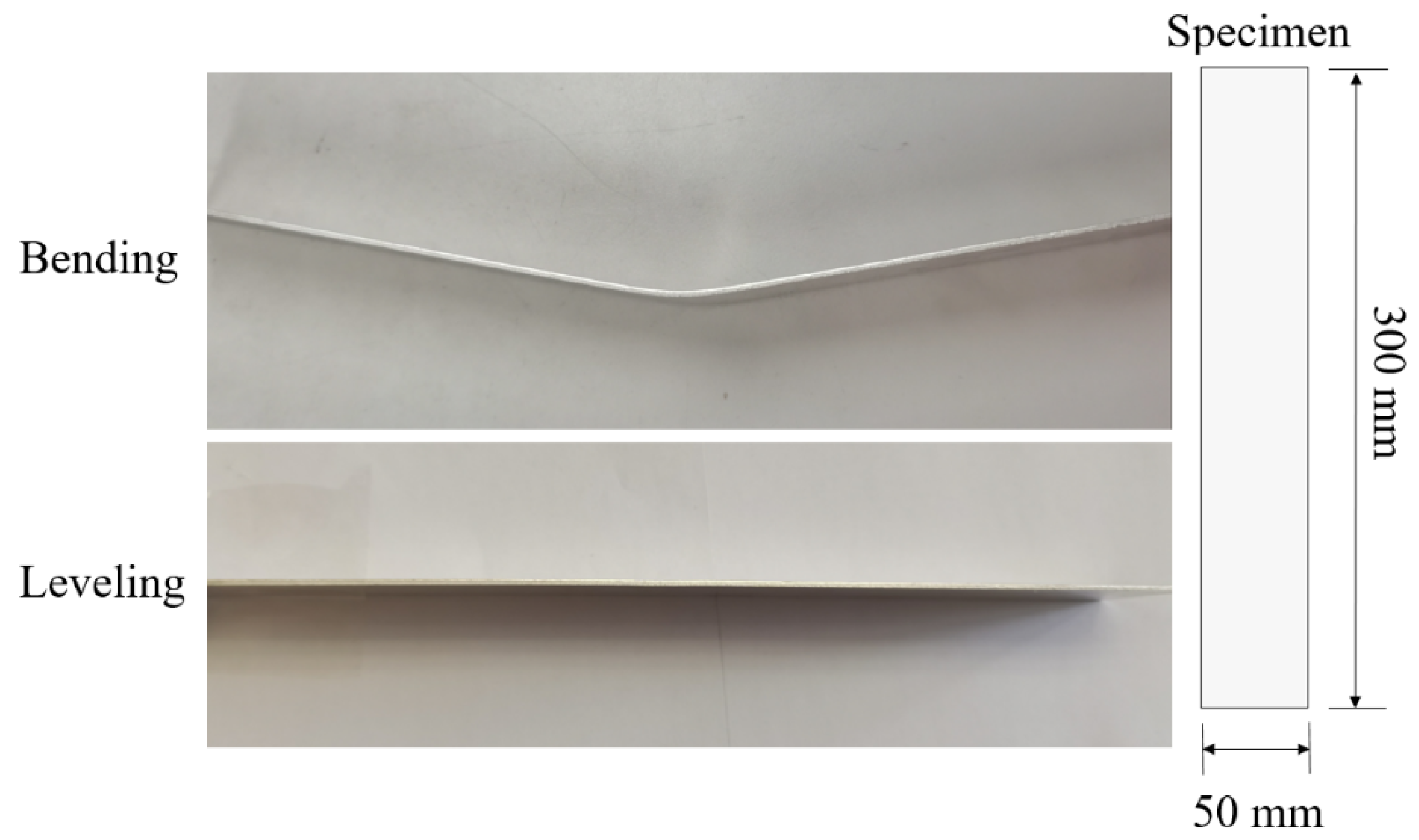
3.4. Experimental Verification
4. Conclusions
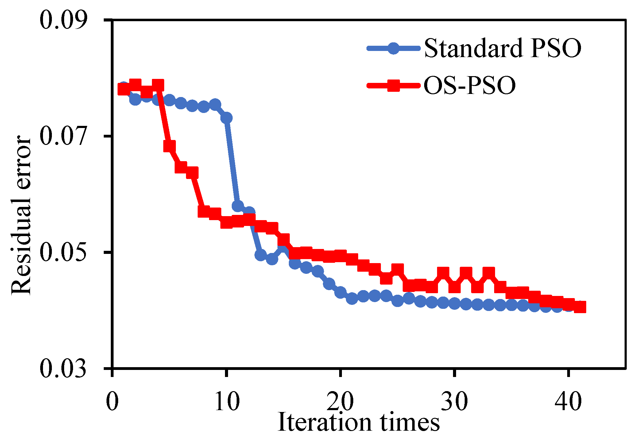
- Improved fitting accuracy is achieved by PSO variation. Compared with GA, the overall residual error was reduced by more than 40% with standard PSO and the standard PSO result was verified by the OS-PSO.
- Local interval accuracy is improved with VW-PSO. With an increased weight in the case of the tensile flow stress interval, the instantaneous Bauschinger effect interval and the permanent softening interval; the interval residual error was reduced by 33% to 40% when compared to standard PSO, while also maintaining a stable overall residual error.
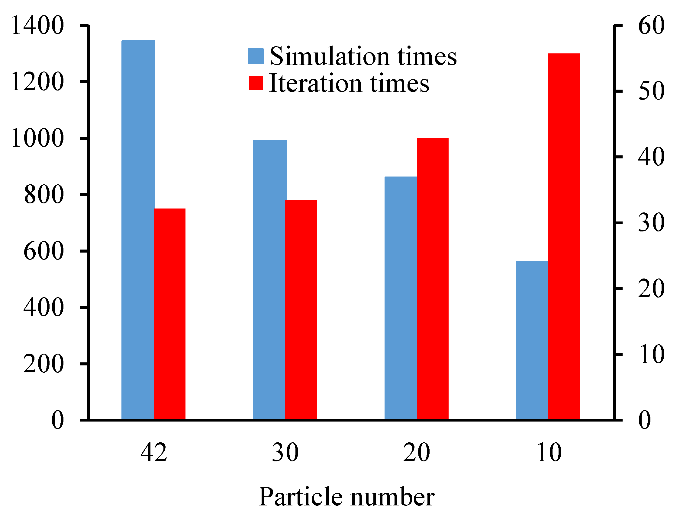
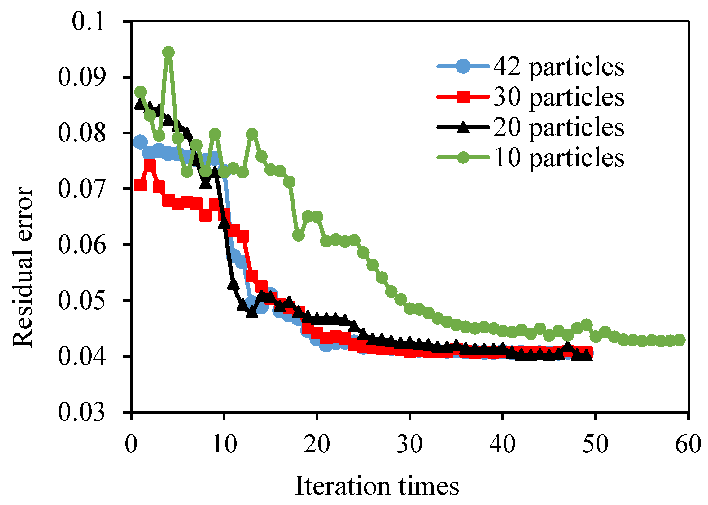
- Computation load and iteration times are cut down by reducing the particle number within a certain range, while also maintaining the overall residual error. In this study, the iteration time and computation load were comparatively low with particle numbers of 20 and 30.
- Acceptable accuracy can be achieved for bending-leveling experiments. The springback prediction errors for both the bending and leveling stages were within 1°.
Author Contributions
Funding
Data Availability Statement
Conflicts of Interest
References
- Olivetti:, E.A.; Cullen, J.M. Toward a sustainable materials system. Science 2019, 360, 1396–1398. [Google Scholar] [CrossRef] [PubMed] [Green Version]
- Worrell, E.; Allwood, J.; Gutowski, T. The role of material efficiency in environmental stewardship. Annu. Rev. Environ. Resour. 2016, 41, 575–598. [Google Scholar] [CrossRef] [Green Version]
- Wang, L.; Guo, Y.Y.; Zhang, Z.L.; Xia, X.H.; Cao, J.H. Generalized growth decision based on cascaded failure information: Maximizing the value of retired mechanical products. J. Clean. Prod. 2020, 269, 122176. [Google Scholar] [CrossRef]
- Zhang, X.G.; Zhang, M.Y.; Zhang, H.; Jiang, Z.G.; Liu, C.H.; Cai, W. A review on energy, environment and economic assessment in remanufacturing based on life cycle assessment method. J. Clean. Prod. 2020, 255, 120160. [Google Scholar] [CrossRef]
- Shi, J.L.; Fan, S.J.; Wang, Y.J.; Cheng, J.S. A GHG emissions analysis method for product remanufacturing: A case study on a diesel engine. J. Clean. Prod. 2019, 206, 955–965. [Google Scholar] [CrossRef]
- Chongthairungruang, B.; Uthaisangsuk, V.; Suranuntchai, S.; Jirathearanat, S. Springback prediction in sheet metal forming of high strength steels. Mater. Des. 2013, 50, 253–266. [Google Scholar] [CrossRef]
- Zang, S.L.; Thuillier, S.; Le Port, A.; Manach, P.Y. Prediction of anisotropy and hardening for metallic sheets in tension, simple shear and biaxial tension. Int. J. Mech. Sci. 2011, 53, 338–347. [Google Scholar] [CrossRef]
- Serkan, T. Parameters determination of Yoshida Uemori model through optimization process of cyclic tension-compression test and V-bending springback. Lat. Am. J. Solids Struct. 2019, 13, 1893–1911. [Google Scholar] [CrossRef] [Green Version]
- Li, J.Q. Parameter calibration of material constitutive model and its application in prediction of bending springback of high-strength steel sheet. Master’s Thesis, South China University of Technology, Guangzhou, China, 2017. [Google Scholar]
- Ghaei, A.; Green, D.E. Numerical implementation of Yoshida-Uemori two-surface plasticity model using a fully implicit integration scheme. Comput. Mater. Sci. 2010, 48, 195–205. [Google Scholar] [CrossRef]
- Yan, J.W.; Hu, Q.; Wang, Z.Z.; Chen, J. A comparison study of different hardening models in springback prediction for stamping of the third generation ultra high strength steel. J. Shanghai Jiaotong Univ. 2017, 51, 1334–1339. [Google Scholar] [CrossRef]
- Phongsai, T.; Uthaisangsuk, V.; Chongthairungruang, B.; Suranuntchai, S.; Jirathearanat, S. Simplified identification of material parameters for Yoshida-Uemori kinematic hardening model. SPIE Proc. 2014, 9234. [Google Scholar] [CrossRef]
- Lee, J.S.; Choi, S.Y.; Lee, S.K.; Song, J.H.; Noh, W.; Choi, S.; Kim, G.H. Roll forming process of automotive seat rail with 980 DP steel using Yoshida-Uemori kinematic hardening model. Procedia Manuf. 2018, 15, 796–803. [Google Scholar] [CrossRef]
- Zhu, J.; Huang, S.Y.; Liu, W.; Zou, X.F. Semi-analytical or inverse identification of Yoshida-Uemori hardening model. Key Engineering Materials 2018, 775, 531–535. [Google Scholar] [CrossRef]
- Leem, A.; Moser, N.; Ren, H.Q.; Mozaffar, M.; Ehmann, K.F.; Cao, J. Improving the accuracy of double-sided incremental forming simulations by considering kinematic hardening and machine compliance. Procedia Manuf. 2019, 29, 88–95. [Google Scholar] [CrossRef]
- Hassan, H.U.; Traphöner, H.; Güner, A.; Tekkaya, A.E. Accurate springback prediction in deep drawing using pre-strain based multiple cyclic stress-strain curves in finite element simulation. Int. J. Mech. Sci. 2016, 110, 229–241. [Google Scholar] [CrossRef]
- Xu, J.; Wang, T.; Rong, Z. Inversion analysis of Yoshida-Uemori material model parameters for high-strength steel based on simulated annealing algorithm. Forg. Technol. 2016, 41, 133–137. [Google Scholar] [CrossRef]
- Shao, J.H.; Li, W.X.; Zhang, H.; Li, X.; Wang, L. Y-U hardening model parameters inversion of aluminum alloy based on second-order oscillatory particle swarm optimization. J. Plast. Eng. 2021, 28, 193–198. [Google Scholar] [CrossRef]
- Yoshida, F.; Uemori, T. A model of large-strain cyclic plasticity describing the Bauschinger effect and workhardening stagnation. Int. J. Plast. 2002, 18, 661–686. [Google Scholar] [CrossRef]
- Hardt, M.; Jayaramaiah, D.; Bergs, T. On the application of the particle swarm optimization to the inverse determination of material model parameters for cutting simulations. Modelling 2021, 2, 129–148. [Google Scholar] [CrossRef]


| Algorithm | Algorithm Description | ||||
|---|---|---|---|---|---|
| Weights | Learning Factor | Update Speed | Update Location | Objective Function | |
| Standard PSO | 1 | c1 = c2 = 2 | Equation (7) | x = x + v | Equation (9) |
| OS-PSO | Equation (10) | Equation (9) | |||
| VW-PSO | Equation (7) | Equation (13) | |||
| Method | cb | Y (MPa) | C | k | Rsat | sb | h | Residual |
|---|---|---|---|---|---|---|---|---|
| Graphical method | 67.31 | 80.87 | 312.23 | 46.98 | 110.35 | 27.99 | 0.4 | 13.09% |
| GA [15] | 99.05 | 79 | 650.22 | 29.49 | 55.06 | 59.21 | 0.3 | 6.84% |
| Standard PSO | 98.27 | 80.87 | 584.87 | 44.05 | 47.16 | 37.00 | 0.4 | 4.01% |
| OS-PSO | 95.35 | 80.87 | 589.50 | 42.37 | 55.14 | 37.61 | 0.4 | 4.05% |
| Interval | cb | Y (MPa) | C | k | Rsat | sb | h | Residual |
|---|---|---|---|---|---|---|---|---|
| interval I | 94.61 | 80.87 | 718.65 | 42.04 | 54.46 | 46.61 | 0.4 | 5.14% |
| interval II | 109.03 | 80.87 | 644.45 | 53.04 | 37.39 | 28.53 | 0.4 | 4.96% |
| interval III | 106.02 | 80.87 | 626.27 | 34.04 | 48.02 | 38.61 | 0.4 | 4.15% |
| Interval | Standard PSO | Variable Weight PSO | Improvement |
|---|---|---|---|
| interval 1 | 4.64% | 3.09% | 33.41% |
| interval 2 | 3.48% | 1.93% | 44.54% |
| interval 3 | 2.95% | 1.61% | 45.42% |
| i | cb | Y (MPa) | C | K | Rsat | sb | h | Residual |
|---|---|---|---|---|---|---|---|---|
| 42 | 98.27 | 80.87 | 584.87 | 44.05 | 47.16 | 37.00 | 0.4 | 4.01% |
| 30 | 97.05 | 80.87 | 607.24 | 46.48 | 46.53 | 38.47 | 0.4 | 4.05% |
| 20 | 98.31 | 80.87 | 582.83 | 49.06 | 50.52 | 32.83 | 0.4 | 4.03% |
| 10 | 101.96 | 80.87 | 517.54 | 43.29 | 49.63 | 33.17 | 0.4 | 4.25% |
| Bending | Leveling | ||||
|---|---|---|---|---|---|
| Bending before rebound | Experiment after rebound | Simulation after rebound | Leveling before rebound | Experiment after rebound | Simulation after rebound |
| 39.6° | 19.3° | 19.5° | 15.9° | 0.6° | 1.6° |
Publisher’s Note: MDPI stays neutral with regard to jurisdictional claims in published maps and institutional affiliations. |
© 2021 by the authors. Licensee MDPI, Basel, Switzerland. This article is an open access article distributed under the terms and conditions of the Creative Commons Attribution (CC BY) license (https://creativecommons.org/licenses/by/4.0/).
Share and Cite
Xia, X.; Gong, M.; Wang, T.; Liu, Y.; Zhang, H.; Zhang, Z. Parameter Identification of the Yoshida-Uemori Hardening Model for Remanufacturing. Metals 2021, 11, 1859. https://doi.org/10.3390/met11111859
Xia X, Gong M, Wang T, Liu Y, Zhang H, Zhang Z. Parameter Identification of the Yoshida-Uemori Hardening Model for Remanufacturing. Metals. 2021; 11(11):1859. https://doi.org/10.3390/met11111859
Chicago/Turabian StyleXia, Xuhui, Mingjian Gong, Tong Wang, Yubo Liu, Huan Zhang, and Zelin Zhang. 2021. "Parameter Identification of the Yoshida-Uemori Hardening Model for Remanufacturing" Metals 11, no. 11: 1859. https://doi.org/10.3390/met11111859
APA StyleXia, X., Gong, M., Wang, T., Liu, Y., Zhang, H., & Zhang, Z. (2021). Parameter Identification of the Yoshida-Uemori Hardening Model for Remanufacturing. Metals, 11(11), 1859. https://doi.org/10.3390/met11111859