Thermographic Analysis of Composite Metallization through Cold Spray

Abstract

Cold Spray is an innovative technology to create coatings through the impact of metallic particles on substrates. Its application to composites’ surfaces is recently attracting the attention of the scientific community thanks to the possibility to functionalize and improve their thermal and wear properties. Within this context, the generation of the first metal-to-composite layer is fundamental. This work presented an experimental investigation of a composite panel, reinforced with glass fibers and coated with aluminum particles. The coating investigation was carried out through active pulsed thermography, analyzing the thermal response of single and double hatches. The thermal outputs were compared with a standard microscopic analysis, with a critical discussion supporting the identification of factors that influence the thermal response to the pulse: (1) layer’s thickness; (2) cold spray coverage; (3) layer compactness; (4) particle-substrate adhesion; (5) particle’s oxidation; and (6) surface roughness.

1. Introduction

Cold Spray (CS) is a recently developed technique suitable for the metallization of different substrates. The deposition occurs through the acceleration of solid-state microparticles towards the target substrate, where the interlocking occurs as a result of the high-velocity impact and the associated severe plastic deformation. The main applications in the literature deal with metal-to-metal coatings to enhance the performance of the coated system regarding wear, corrosion, fatigue, etc. [1,2]; CS has also been suggested for additive manufacturing of freestanding parts [3,4]. However, recently, attention is also moving towards metal-to-composites with polymers or polymeric matrix composites substrates; this last application is known as polymer metallization. Metallic coatings aim to functionalize and improve the composites’ thermal and electrical properties [5] and wear and erosion resistance [6], but they can also act as electromagnetic shielding and as lightning strike protection in the aerospace industry [7]. Polymer metallization using CS has several advantages compared with some counterparts as metal sheet bonding, electroless plating, physical and chemical vapor deposition, and thermal spray techniques. In particular, we can mention [8]: (1) the reduction of processing costs due to high build-up rate, (2) the possibility to achieve higher coating thicknesses, (3) the reduction of metal oxidation that occurs with any thermal process at high temperatures, (4) the reduction of substrate degradation thanks to the lower temperature, and (5) the possibility to avoid size limitations of the component as there is no need for an environmental chamber and the spraying device is mounted on a robot, allowing for a full 3D deposition.

There are some literature studies on successful polymer metallization focused on thermoplastics such as PE (polyethylene), PEEK (polyether ether ketone), and PEI (polyethylenimine) [9,10], because the deposition on thermoset polymers has proved to be quite difficult due to erosion phenomena under the supersonic particle velocity using cold spray [11,12]. The only metal which was successfully cold sprayed on thermosets was reported to be tin and its blends due to their incipient melting during deposition [13]. A practical solution to low cold sprayability of thermosets is to place a thin thermoplastic layer on the substrate surface before deposition [14]. These works showed that the particle velocity must be selected properly within a deposition window by tuning the processing parameters. In particular, for a successful deposition of the first metal-to-composite layer, corresponding to the beginning of the coating’s growth, the velocity must be higher than the interlocking velocity of particles with the polymeric substrate, but lower than the erosion velocity of the polymer itself, as proved through experiments analyzing the whole coated layer [9,15] and the single-particle impact [16], as well as with complex numerical simulations [17,18].

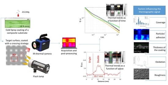
This study aimed to characterize the first layers of a cold-sprayed composite panel through pulsed infra-red (IR) thermography [19]. This non-destructive (ND) and non-contact experimental technique is classified as active thermography. Indeed, it requires external thermal stimulation, typically heating, of the tested component, in opposition to passive thermography wherein self-heating occurs as a consequence of the applied loads. This load-dependent thermal behavior was related to the fatigue limit of the material, including composites [20,21,22].

Active thermography has been widely used in the literature for the inspection of metal-to-metal coatings. For instance, to cite a few works, Moskovchenko et al. [23] determined the thickness of a Cr coating on an S235 substrate based on the thermal effusivity, with a 20% maximum error in the range 0.1–1.1 mm compared to microscopic analysis. Tang et al. [24] investigated SiC thermal-barrier coatings on superalloy specimens, comparing experiments with a heat conduction analytical model, finding good estimations in the range of 40–120 μm coating thickness. Bu et al. [25] also investigated thickness and delamination with pulsed thermography combined with a simulated annealing algorithm, finding less than 10% error in the range 45–130 μm. Shrestha et al. [26,27] combined pulsed and lock-in thermography [28] for the experimental and numerical analysis of a 0.1–0.6 mm thick topcoat in Yttria-stabilized Zirconia on a Ni-based superalloy, with errors lower than 17%. Besides, Tamborrino et al. [29] described the measurement of a WC-Co-Cr coating thickness obtained from thermal spraying, comparing traditional pulsed thermography with a novel approach called long pulse thermography, return values with a precision of one-hundredth of a millimeter.

Regarding polymer composites, the application of pulsed thermography has dealt with the identification of manufacturing or induced defects, such as drilled holes [30] and delamination by impacts [31]. However, due to the recent developments of CS on composites, to the best of the authors’ knowledge, there are still no thermographic studies on metallic coatings applied to composites.

The focus of this work was on the thermal surface response after a heat pulse, critically discussing how it is influenced by different manufacturing factors, such as the thickness and coverage of the coated layer, as well as adhesion and oxidation of the particles. Besides, the thermographic findings were compared to a standard microscopic analysis with the Scanning Electron Microscope (SEM), followed by a critical discussion.

Before presenting the experimental methodology and the results, we present here in the introduction a brief overview of the processing techniques for the pulsed thermography implemented in the literature, with related equations.

Thermal-Image Processing Techniques

The literature developed several image processing techniques to analyze surfaces with active IR thermography [32,33], often aimed at the inspection and detectability of manufacturing or load-induced defects. Some works [30,34] classified them in: (1) thermal contrast techniques, with differential absolute or interpolated differential absolute contrasts [35,36]; (2) techniques based on transforms from the time to the frequency domains, such as the pulsed phase thermography [37,38]; and (3) techniques using statistical methods, including the Thermal Signal Reconstruction (TSR) and its derivatives [39,40], developed to decrease the time noise. The selection of the most suitable processing techniques has been under debate within the thermographic community because it depends on the objectives and needs of the specific study. For instance, the thermal contrast techniques were mainly introduced to detect defects, e.g., ND testing, comparing the thermal trends of a reference area without defects with an area with defects. These approaches are less meaningful in the case of sprayed panels, where different coated and uncoated areas are present at the surface. Besides, transform-based techniques require specific setups of the devices to analyze the periodic transient heating signal. On the other hand, statistical methods are easily implementable with pulsed thermography and a simple test setup.

Processing the thermal signal aims to reduce data as well as noise with filtering. The TSR technique has its origin in the Fourier’s one-dimensional heat-transfer equation on a semi-infinite homogeneous surface previously subjected to thermal excitation (Dirac delta). Surface temperature, e.g., the thermal evolution of a pixel $T\left(t\right)$, is modeled in the logarithmic scale with a ½ slope with the following equation [41]:

$$ln\left[T\left(t\right)\right]=ln\left(\frac{Q}{e}\right)-\frac{1}{2}ln\left(\pi t\right)$$

(1)

where $T$ is the measured surface temperature at a pixel, $t$ is the time, $Q$ is the energy absorbed by the surface and, $e$ is the material effusivity. This equation can be also interpolated with a polynomial function of degree $n$:

$$ln\left[T\left(t\right)\right]=a_0+a_{1}ln\left(t\right)+a_2{ln}^2\left(t\right)+\cdots +a_n{ln}^n\left(t\right)$$

(2)

where the coefficients $a$ can be obtained from least-squares fitting. With this equation, the image sequence information is reduced to these $n$ coefficients used in the reconstruction. The choice of the polynomial order $n$ is crucial since high $n$ provides oscillating thermal reconstruction while reducing denoising; on the other hand, small $n$ prevents a smooth fit. According to some works in the literature [38,40,42], the choice of $n$ equal to 4 or 5 is sufficient to act as a low pass filter, smoothening the thermal trend.

The derivatives of the polynomial TSR in the double logarithmic scale allow detecting the maximum contrast in early time [43], which could be particularly interesting for the case of CS coatings. The first and second derivatives of the TSR have these expressions, respectively [40]:

$$\frac{d\left[lnT\left(t\right)\right]}{d\left[ln\left(t\right)\right]}={\displaystyle \sum }_{i=1}^{n}i{a}_i{\left[ln\left(t\right)\right]}^{i-1}$$

(3)

$$\frac{d^2\left[lnT\left(t\right)\right]}{d{\left[ln\left(t\right)\right]}^2}={\displaystyle \sum }_{i=1}^{n}i\left(i-1\right)a_i{\left[ln\left(t\right)\right]}^{i-2}$$

(4)

These equations can be applied to the raw thermograms in the time domain, as well as to the normalized thermal images. Normalization is a post-processing analysis carried out to reduce the effects of non-uniform excitation and surface emissivity. In the thermographic literature, one of the most accepted is the standardization proposed by Rajic [44]. At a fixed time, the normalized standard response of a pixel is calculated as:

$$\widehat{T}\left(j,k,t\right)=\frac{T\left(j,k,t\right)-\overline{T}\left(j,k\right)}{{\sigma }_{T\left(j,k\right)}}$$

(5)

where j and k are the variables spanning row and columns of the thermal matrix, and $\overline{T}\left(j,k\right)$ and ${\sigma }_{T\left(j,k\right)}$ are the mean value and the standard deviation of each pixel over time, respectively.

In the present study, we propose another normalizing function:

$$\widehat{T}\left(j,k,t\right)=\frac{T\left(j,k,t\right)-T\left(j,k,t=0\right)}{T\left(j,k,t=1\right)-T\left(j,k,t=0\right)}$$

(6)

where, considering a sequence of acquired images, of which at least one is taken before the flash, $T\left(j,k,t=0\right)$ is the temperature of the processed pixel before the flash, $T\left(j,k,t=1\right)$ is the temperature of the processed pixel of the first image acquired after the flash, and $T\left(j,k,t\right)$ is the temperature of the processed pixel at the general time t.

Considering that the IR signal can be affected by a reflection of external sources and by non-uniform heating of the source or by a non-uniform thermal emissivity, the subtraction eliminates the reflected component, while the ratio eliminates the non-uniform surface heating or emissivity after the flash.

2. Materials and Methods

A composite panel made of E-Glass Fibre reinforcement (twill 2/2 fabric, Hexcel composites, Stamford, CT, USA) and low-viscosity epoxy matrix SX10 EVO (by Mates Italiana, Segrate, Italy) was manufactured by vacuum-assisted resin infusion. A polypropylene (PP) thermoplastic layer was primarily hot compacted at 165 °C with the E-Glass Fibre reinforcement monolayer to form a composite top surface for the metallization operation. This top layer is necessary to assist and enhance the sprayed particle interlocking, as discussed in the introduction. During the hot compaction, the desirable condition was the partial impregnation of the thermoplastic resin into the fibre layer. In the following stage of resin infusion, the adhesion enhancement was anticipated by means of a cocuring action between the PP thermoplastic layer in the preform and the infused epoxy resin through the E-glass reinforcing layers [14,45]. The total thickness of the E-glass and epoxy composite laminate was approximately 2.8 mm, obtained from eight layers of glass fabrics; the volume fraction was 0.4. The top layer of PP was 500 μm thick; the panel size was 200 × 200 mm.

The surface metallization of the composite panel was performed with low-pressure CS equipment (Model D423, by Dycomet, Obninsk, Russia) using AlSi10Mg powder with a spherical shape of 20 μm average diameter. The following CS parameters were used: gas temperature of 250 °C and gas pressure of 6 bar, Stand-off Distance (SoD) of 45 mm, nozzle advancement speed of 1 mm/s, and Powder Feeding Rate (PFR) of 5 g/min. The spraying strategy used for the panel followed the x-y directions: at first, horizontal hatches (x-axis) were sprayed, followed by the vertical ones (y-axis), creating a periodic and regular squared pattern. The distance between the hatch axes was 20 mm, allowing us to leave some PP clearly uncoated at the surface. Indeed, the width of the hatches was about 15 mm, as visible by the naked eye and as which is discussed later in detail in the results section.

Further details regarding the manufacturing of the panel object of this work are described in [14,45]. Eventually, after these manufacturing steps, the final composite was made of four different materials: (1) glass fibres, (2) epoxy resin, (3) polypropylene, and (4) aluminum coating.

The experimental technique of active pulsed thermography was selected to analyze the effective coating of the panel. A 300 W halogen lamp (Model Style RX 1200, by Elinchrom, Renens, Switzerland) with flash duration 1/1450 s was employed as the thermal source. The flash (and consequently the thermal heating) was almost instantaneous and homogeneous over a region of interest (ROI), selected as a representative part of the squared pattern generated by the hatches. The ROI included both uncoated PP as well as single and double hatches.

Surface temperature at the ROI was collected by an IR camera (Model Cedip-FLIR Titanium by FLIR Systems, Täby, Sweden) with an InSb sensor having a NETD equal to 25 mK. This IR camera allows acquiring thermal images at a maximum of 160 Hz with a full frame (320 × 265 pixels), and it reached 472 Hz, reducing the window to 160 × 128 pixels. Some preliminary tests allowed selecting this second option as the best one to analyze the sprayed coating pattern, and the camera was placed at a distance from the panel, resulting in a spatial resolution of 0.1875 mm/pixel. Figure 1 schematizes the test setup. Temperatures at each pixel were stored as a function of the time on a laptop, connected via an Ethernet cable with the IR camera. Data storage was performed with the software Altair by FLIR Systems (v.5.90.002, Täby, Sweden); the flash occurred 0.2 s after the beginning of the recording and the total recording time was 1.7 s.

After the thermal measurements, the panel was cut with a vertical saw in correspondence with the ROI to allow observations and measurements at the SEM (Model EVO 50XVP by Zeiss, Oberkochen, Germany). The SEM was operated at a working voltage of 20 kV along with a proper working distance for a focused image using the secondary electron (SE) detection. Two samples were extracted with a band saw, as shown in Figure 2: the line in between the two samples corresponds to the axis of a horizontal hatch. S1 was used for a through-thickness analysis along the axis of the hatch (lower side), while S2 allowed for analyzing the surface and its coverage. The size of the embedded particles was measured from these SEM images in terms of equivalent diameter using the software MATLAB (version R2018a, MathWorks, Natick, MA, USA). Eventually, to support the discussion, the SEM was also used to perform a chemical analysis at the surface of the coating using energy-dispersive X-ray spectroscopy (EDS), focusing on the presence of oxygen. The SEM had a resolution of 0.1% for the measurements of elements’ concentrations; chemical measurements were repeated over 4 areas on the axis of the horizontal hatch and of the vertical hatch, far from the crossing. The concentration results were processed with the boxplot command of the software MATLAB.

3. Results

Figure 3 shows the recorded raw and normalized thermograms of the ROI at the first four frames after the flash; the normalization is obtained from Equation (6).

Given that the stored data embed four variables (temperature T, time t, and distance along the horizontal and vertical axes), the thermal trends were plotted first in the time domain and then in the space, e.g., at each pixel.

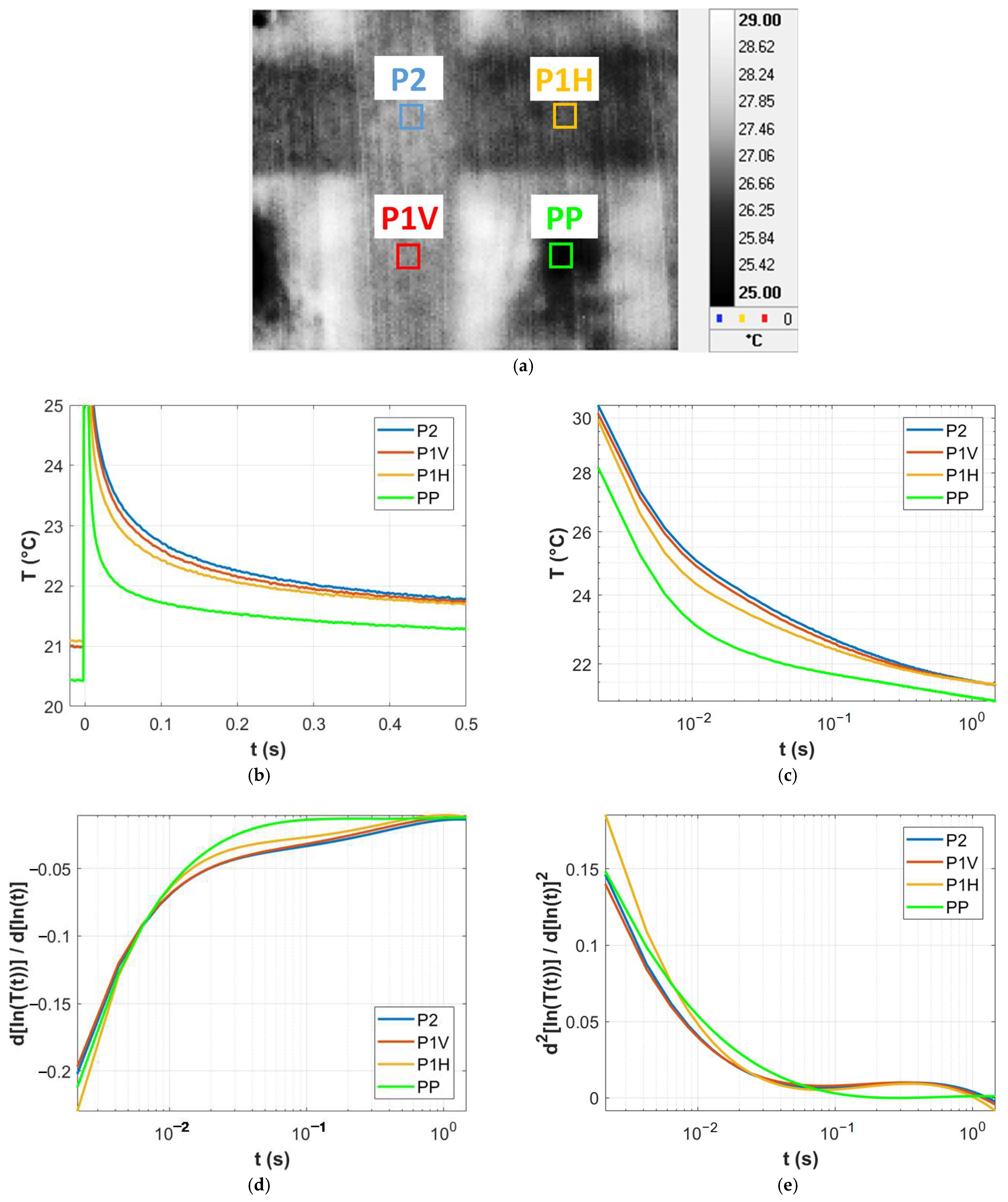
Figure 4 and Figure 5 analyze the raw and the normalized thermograms, respectively. Thermal data were extracted and averaged over four squared regions with size 10 × 10 pixels, shown in Figure 4a and Figure 5a. They correspond to: (1) the double hatches (P2), e.g., the region where horizontal and vertical hatches cross; (2) the horizontal single hatch (P1H); (3) the vertical single hatch (P1V); and (4) the uncoated PP. Figure 4b,c and Figure 5b,c plot the thermal trends in linear and logarithmic scale of these regions as a function of time, while Figure 4d,e and Figure 5d,e show the trends of the first and second derivatives of the TSR, calculated from Equations (3) and (4) respectively.

Figure 6 and Figure 7 analyze the raw and the normalized thermograms at a fixed frame (time). These plots describe the thermal trend in the space, along the four profiles shown in Figure 5a and Figure 6a: (1) H1, crossing the single vertical hatch; (2) H2, centered in the horizontal hatch; (3) V1, crossing the single horizontal hatch; and (4) V2, centered in the vertical hatch. Surface temperatures are given as a function of the distance along the profiles, as raw (Figure 5b–e) and normalized values (Figure 6b–e). The repeatability of the data plotted in Figure 6 and Figure 7 was statistically checked, both repeating the tests with the same setup, as well as selecting the profiles with a ±5 pixel offset from the selected position, e.g., checking the effect of the position. In all cases, the confidence bounds were very limited and almost overlapped to these same plots.

After this thermographic analysis, the samples S1 and S2 were cut from the panel for microscopic analyses. The sample S1 was embedded into resin for the through-thickness analysis, performed in the five points shown in Figure 8a; point 3 is in correspondence of the axis of the vertical and horizontal hatches, e.g., crossing point, while points 2 and 4, and points 1 and 5 were located at a symmetrical distance with respect to the axis of the vertical hatch. Figure 8b–e show the images collected at the Scanning Electron Microscope (SEM).

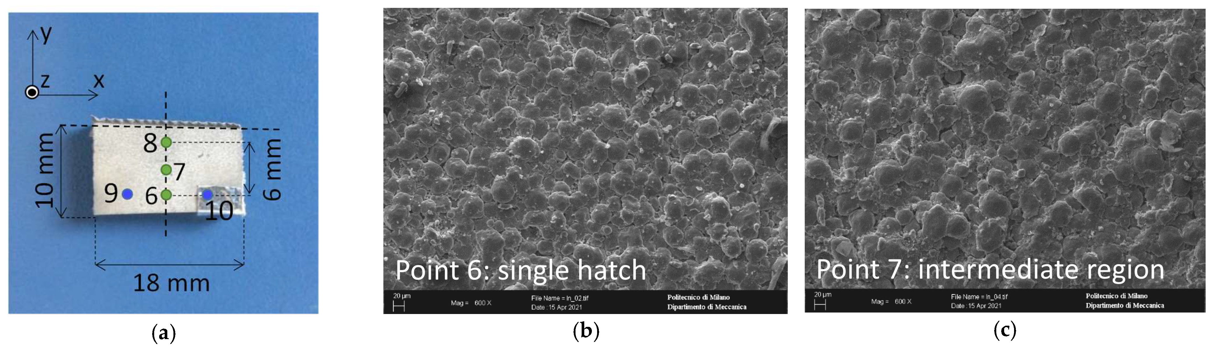
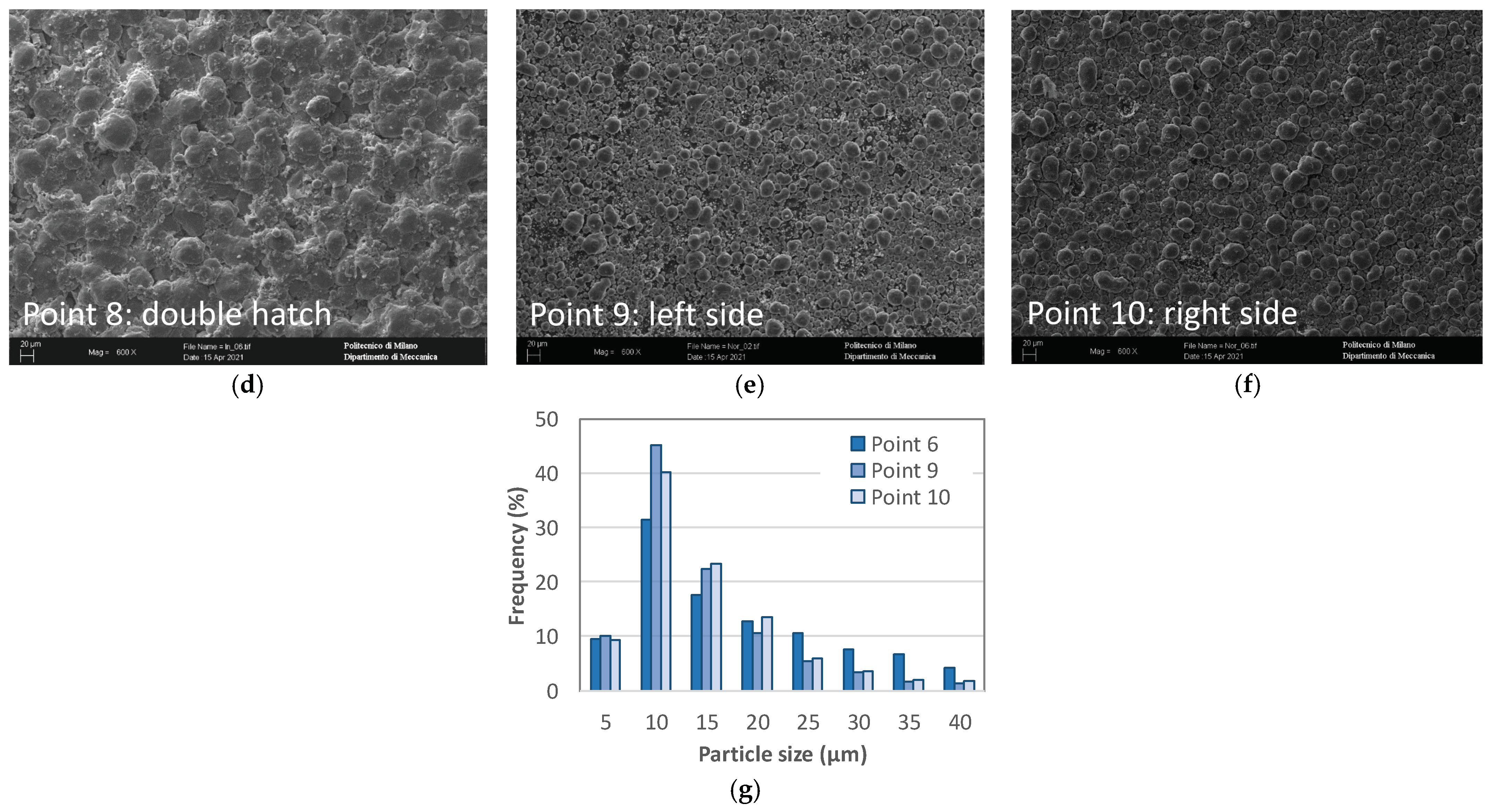
On the other hand, the coated surface of sample S2 was directly observed, see Figure 9a, for points identification. points 6, 7, and 8 lay along the vertical hatch, at an increasing distance from the horizontal hatch. Eventually, points 9 and 10 were at the side region of the vertical hatch, but not in the uncoated region, which is not the main focus of this study. They were the only ones out of the axis of any hatch.

4. Discussion

4.1. Thermal Trends as a Function of the Time

Within the ROI, differences in the thermal response can be observed easily in Figure 3 from the raw thermograms as a function of the time. Already from these thermal images, it is evident that the horizontal hatch cooled down more quickly than the vertical one, which was the secondly performed one.

It seems that both the first horizontal and the second vertical hatches also affected the surface of the sample outside the hatch itself, where the particles are successfully interlocked. In other words, some powder was left on the sample surface outside the hatch itself due to the deposition process. This is confirmed by the slow temperature decay of the two regions on the left and right sides of the second and last vertical hatches.

This is also confirmed by the SEM images of Figure 9, which will be later discussed in detail. Here, we briefly recall Figure 9g; this histogram shows that points 9 and 10 at the side of the hatch were characterized by a greater number of small particles with a diameter equal to or less than 10 μm when compared with point 6 at the center of the hatch. These small particles may not be well-adhering to the substrate. The powder created on the sides of the first horizontal hatch was then embedded under the second hatch during its deposition process. This explains why the features of the second vertical hatch seem different from those of the first horizontal hatch; the part of the second hatch superimposed or crossing the first horizontal hatch gives a thermal response similar to the non-superimposed region. This means that the powder on the sides of the first horizontal hatch created an extra layer under the second vertical hatch. We suppose that this is the reason why the thermal time decay of the second vertical hatch was almost homogeneous regardless of the presence of the first hatch underneath.

The powder left at the edges of the first horizontal hatch then formed an extra layer under the second vertical hatch, which in turn also left two layers of powder at its edges, while eliminating the powder left by the horizontal hatch not directly underneath the vertical hatch.

The normalized images of Figure 3 enhance these local differences, already visible from the raw images. Both the raw and the normalized images showed the powder at the edges of the second vertical hatch as a region with a slower temperature decay than the rest of the sample surface.

To deepen these initial observations, local analyses were performed selecting the regions of Figure 4a and Figure 5a. Let us discuss at first the results from the raw thermograms of Figure 4, at the frame corresponding to t = 2/472 s when the difference between the vertical and the horizontal hatches started being more evident. The temperature trends are plotted as a function of the time in the linear scale of Figure 4b, as well as in the logarithmic scale of Figure 4c to enhance their differences. The polypropylene PP was the coldest region; indeed, not only did it reach lower temperatures during the flash, but also it experienced a thermal trend always lower than the other analyzed regions. This experimental evidence can be explained considering that the thermal energy deposited on the polymer surface by the flash pulse is absorbed within a volume directly under the surface because the polymer is semi-transparent to the radiation. The center of the double hatch P2 and the center of the vertical hatch P1V showed a very similar thermal trend as a function of time. On the contrary, P1H, which was at the center of the horizontal hatch, showed a faster temperature decay. This is opposite to what one could expect, i.e., that the vertical and the horizontal hatch should behave in the same way, when not superimposed, because the parameters of the deposition are the same.

The hypothesis given above, i.e., that the powder left at the edges of the first horizontal hatch was trapped underneath the second vertical hatch and formed an extra layer under the vertical hatch only, explains well the uniform thermal behavior of the vertical hatch, on and outside the horizontal hatch.

Obviously, all these coated regions were hotter than the PP, because the thermal energy was mainly absorbed on the surface, where the Al particles are deposited, and within a volume, where the polymer appeared directly on the surface.

Apparently, the raw thermal trends of Figure 4b,c are similar to the normalized trends of Figure 5b,c. Here, the time selected for the analysis is already the first frame, i.e., t = 1/472 s, because the difference among the regions is immediately evident. When the thermograms were processed and normalized, the obtained decaying trends were similar to the raw ones. This may be explained considering that, though the emissivity of polished Al is quite low, the emissivity of this Al layer was quite high because it was formed by oxidized Al particles, creating a rough surface.

Only the PP experienced, for the normalized trend of Figure 5c, a wavy trend not visible from the unprocessed data; this does not depend on its different emissivity, but rather on the volume absorption of the light emitted by the flash.

The first and second derivatives of the logarithmic TSR as a function of the time were calculated from Equation (3) and (4), and plotted in Figure 4d,e and Figure 5d,e. The analysis of these trends led to similar conclusions on the different thermal responses of the four analyzed regions. In addition, we can add some further comments: the first derivative of the raw TSR (Figure 4d) did not experience a maximum, and the second derivative (Figure 4e) was never equal to zero unless at the end of the scanned time, i.e., there is not an inflection point in Figure 4c. In other words, the difference in the thermal behavior among the analyzed regions is more difficult to distinguish when focusing on raw thermograms. On the other hand, when considering the normalized logarithmic plot of the TSR (Figure 5c), its derivatives clearly evidenced the inflection points occurring sooner for the coated regions than for the polymer. Hence, the derivatives’ analysis, which is more sensitive to thermal changes than the raw thermograms, helps in the comparison of the different trends and allows detecting the differences of the regions more precisely.

4.2. Thermal Trends as a Function of the Distance

This subsection focuses on the surface thermal trends at a fixed time, discussing the results of Figure 6 and Figure 7 along four characteristic profiles.

Let us start from the raw profiles of Figure 6. Along H1 (Figure 6b), crossing the vertical hatch, there were: (1) the colder region of PP at its extremities, in accordance with Figure 4; (2) two spikes of temperature at the side of the hatch, where there were some smaller particles, not adhering to the substrate and getting very hot because they did not transmit thermal energy to the substrate; and (3) a flat trend, 5.8 mm in width, identifying the region where the hatch had homogeneous thermal behavior. This latter measure suggests the effective width of the coating, e.g., where we can expect similar properties in coverage and thickness. Similar information can be drawn from V1 (Figure 6d), showing a width of the hatch equal to 7.9 mm, but with much less powder at the edges. On the other hand, H2 and V2 profiles (Figure 6c,d) followed the hatches’ axes. While V2 was almost flat, H2 showed a difference where the two hatches were superimposed.

The normalized plots of Figure 7 support these considerations. From H2 and V2 (Figure 7c,e), we can infer that the measures of the hatches’ width are similar between the raw and the normalized profiles.

4.3. SEM Analysis

Figure 8 shows some SEM images collected at five points along profile H2; all these points belong to the hatch, according to its width measurement in Figure 7c. Even if one can expect differences among point 3 on the one hand, and points 1 and 5 on the other, i.e., the center of the double hatch and the region with only one hatch, the SEM measurements revealed that the thickness of the coating was similar. The measurements indicate a thickness between 30 and 40 μm, with a peak of 58 μm. There are particles of different sizes at different points. However, particles of smaller sizes were often below particles with a higher diameter (dashed circle in Figure 7d). This can suggest that smaller particles underwent higher acceleration in the CS nozzle, reaching the surface before the others. It is likely that these smaller particles help in the creation of the first layer, increasing the roughness of the substrate and the interlocking of the subsequent impacts. Experimental observations suggest also an alternative possibility, i.e., that smaller particles impacting after the bigger ones can fill up the void spaces in between them (dashed circle in Figure 7b). This could be an explanation for the missing growth of the coating, e.g., none of the images showed a double layer even where the two hatches were superimposed. Indeed, before the layer thickness starts increasing through a metal-to-metal deposition, the first layer interlocked with the polymer should be uniform not only in coverage and thickness but also in compactness.

The surface analysis along profile V2 suggests a full coverage in any point of the axis (points 6, 7, and 8 of Figure 9b–d). The difference in the thermographic signal between these points underlines that only the coverage was not sufficient to describe the coating efficiency, e.g., the only upper-view of the sprayed coating could not give full information on the coating itself. Hence, we can state that only the mutual influence of coverage, thickness, and compactness justifies the thermographic trends along the profiles H2 and V2 (Figure 6c,e and Figure 7c,e).

Scanning profile H1 and the points 9 and 10 of Figure 9e,f showed full coverage obtained with particles of smaller size, compatible with the commonly Gaussian deposition profile of the feedstock flow during deposition CS [46]. More in detail, point 6 had particles with bigger sizes, up to an equivalent diameter of 40 μm, while points 9 and 10 were similar and coated with smaller particles, almost 40–45% of them having a diameter around 10 μm, i.e., lower than the average size of the sprayed particles. This finer particle size at the borders of the hatch, not fully adherent to the polymer, justifies the thermographic signal with the side spikes along H1 of Figure 6b and V1 of Figure 6d. The IR camera analyzed an average trend, being unable to see the single particles.

A chemical analysis was also performed with the SEM on two regions, at the axes of the horizontal and of the vertical single hatches. These measurements resulted in the oxygen concentrations of Figure 10. Despite their being quite low (median values: 2.04% for the horizontal hatch, and 1.37% for the vertical hatch) and that the confidence intervals were intersecting, we can underline that the horizontal hatch almost had a double oxygen concentration, hence suggesting some oxidation phenomena. This may be explained qualitatively considering that the deposition of each hatch leaves, at its edges, smaller powder particles. The last deposited hatch, in this case the vertical one, left these smaller particles on the horizontal one, having a larger surface than the bigger particles at the center of the vertical hatch. It is likely that this determined a higher oxygen level at the surface.

5. Conclusions

We can summarize the findings obtained from the experimental comparison between the pulsed thermography and the SEM analysis as follows:

• The light of the flash used as a heat source in pulsed thermography was absorbed on the surface, where the surface is coated by metal particles, while it was absorbed in a volume where the polymer appears uncoated. This determined the lower heating of the polymer visible in every IR image.
• SEM images of a section of the sample showed that the cold spray of metal particles homogeneously covered the surface, but did not result in a double thickness of the coating where the two hatches were superimposed.
• Particles of smaller diameter were observed at the edges of the vertical hatch, which was also the last one to be deposited. IR images showed a slower thermal decay of the temperature of these regions with time. This can be interpreted with the fact that these smaller particles formed a powder layer not perfectly adhering to the polymeric substrate.
• Such a powder layer was not detected at the edges of the first deposited horizontal hatch. This can be interpreted by supposing that the subsequent cold spray deposition of the vertical hatch removed the powder left during the previous deposition of the horizontal hatch.
• The thermal decay with time on the axis of the vertical hatch was similar everywhere, no matter if there was the superimposition with the horizontal hatch or if the analyzed region was far away from it. This can be explained considering that the deposition of the horizontal hatch left, at its edges, some powder, which remained underneath the second hatch when it was deposited, being embedded with it. On the contrary, no powder was on the surface of the sample at the time of the deposition of the first horizontal hatch. This explains why the horizontal hatch showed a difference in the regions where it crossed the vertical hatch compared with regions where the horizontal hatch was alone.
• The results of the chemical analysis, revealing a higher oxygen concentration in the horizontal hatch, can be explained considering that the powder left at the edges of the vertical hatch was also left on the horizontal hatch. This powder, formed by Al particles of smaller diameter, exposed a larger surface to the oxidation caused by the second hatch.
• In conclusion, we identified some factors influencing the response of this panel to a flash pulse: (1) the thickness of the deposited layer; (2) the cold spray coverage; (3) the compactness of the layer; (4) the adhesion of the particles to the substrate; (5) the particle’s oxidation; and (6) the surface roughness, also induced by particles’ size. They are the main parameters factors that should be checked to assess the successful deposition of the first layer of the coating.

All the observations obtained with the IR pulsed thermography, the SEM, and the chemical analysis are consistent with the explanation given above. Hence, thermography has some interesting potentialities to analyze thermal coatings and their deposition.

Future works should address verifying these hypotheses, for instance, removing the smaller and non-adherent particles after each hatch. Such particles, left by the deposition process, significantly affected the results obtained in this work, but should be of little or no importance in the mechanical features of a component, which are the aim of such a metal deposition procedure. Further work should be also devoted to attainment of thicker layers made from multiple hatches, as well as to the most suitable techniques, such as pulsed thermography, to characterize them.

References

- Ghelichi, R.; MacDonald, D.; Bagherifard, S.; Jahed, H.; Guagliano, M.; Jodoin, B. Microstructure and fatigue behavior of cold spray coated Al5052. Acta Mater. 2012, 60, 6555–6561. [Google Scholar] [CrossRef]
- Jones, R.; Kovarik, O.; Bagherifard, S.; Cizek, J.; Lang, J. Damage tolerance assessment of AM 304L and cold spray fabricated 316L steels and its implications for attritable aircraft. Eng. Fract. Mech. 2021, 254, 107916. [Google Scholar] [CrossRef]
- Terrone, M.; Ardeshiri Lordejani, A.; Kondas, J.; Bagherifard, S. A numerical approach to design and develop freestanding porous structures through cold spray multi-material deposition. Surf. Coat. Technol. 2021, 421, 127423. [Google Scholar] [CrossRef]
- Bagherifard, S.; Kondas, J.; Monti, S.; Cizek, J.; Perego, F.; Kovarik, O.; Lukac, F.; Gaertner, F.; Guagliano, M. Tailoring cold spray additive manufacturing of steel 316 L for static and cyclic load-bearing applications. Mater. Des. 2021, 203, 109575. [Google Scholar] [CrossRef]
- Lomonaco, P.; Weiller, S.; Feki, I.; Debray, A.; Delloro, F.; Jeandin, M.; Favini, B.; Rossignol, C. Cold spray technology to promote conductivity of short carbon fiber reinforced polyether-ether-ketone (PEEK). Key Eng. Mater. 2019, 813, 459–464. [Google Scholar] [CrossRef]
- Perna, A.S.; Viscusi, A.; Astarita, A.; Boccarusso, L.; Carrino, L.; Durante, M.; Sansone, R. Manufacturing of a metal matrix composite coating on a polymer matrix composite through cold gas dynamic spray technique. J. Mater. Eng. Perform. 2019, 28, 3211–3219. [Google Scholar] [CrossRef]
- Che, H.; Gagné, M.; Rajesh, P.S.M.; Klemberg-Sapieha, J.E.; Sirois, F.; Therriault, D.; Yue, S. Metallization of carbon fiber reinforced polymers for lightning strike protection. J. Mater. Eng. Perform. 2018, 27, 5205–5211. [Google Scholar] [CrossRef]
- Parmar, H.; Tucci, F.; Carlone, P.; Sudarshan, T.S. Metallisation of polymers and polymer matrix composites by cold spray: State of the art and research perspectives. Int. Mater. Rev. 2021, 1–25. [Google Scholar] [CrossRef]
- Che, H.; Chu, X.; Vo, P.; Yue, S. Metallization of various polymers by cold spray. J. Therm. Spray Technol. 2018, 27, 169–178. [Google Scholar] [CrossRef] [Green Version]
- Bobzin, K.; Wietheger, W.; Knoch, M.A. Development of thermal spray processes for depositing coatings on thermoplastics. J. Therm. Spray Technol. 2021, 30, 157–167. [Google Scholar] [CrossRef]
- Che, H.; Vo, P.; Yue, S. Metallization of carbon fibre reinforced polymers by cold spray. Surf. Coat. Technol. 2017, 313, 236–247. [Google Scholar] [CrossRef] [Green Version]
- Affi, J.; Okazaki, H.; Yamada, M.; Fukumoto, M. Fabrication of aluminum coating onto CFRP substrate by cold spray. Mater. Trans. 2011, 52, 1759–1763. [Google Scholar] [CrossRef] [Green Version]
- Che, H.; Chu, X.; Vo, P.; Yue, S. Cold spray of mixed metal powders on carbon fibre reinforced polymers. Surf. Coat. Technol. 2017, 329, 232–243. [Google Scholar] [CrossRef]
- Parmar, H.; Gambardella, A.; Perna, A.S.; Viscusi, A.; Della Gatta, R.; Tucci, F.; Astarita, A.; Carlone, P. Manufacturing and metallization of hybrid thermoplastic-thermoset matrix composites. In Proceedings of the ESAFORM 2021 24th International Conference on Material Forming, Liège, Belgium, 14–16 April 2021. [Google Scholar]
- Gillet, V.; Aubignat, E.; Costil, S.; Courant, B.; Langlade, C.; Casari, P.; Knapp, W.; Planche, M.P. Development of low pressure cold sprayed copper coatings on carbon fiber reinforced polymer (CFRP). Surf. Coat. Technol. 2019, 364, 306–316. [Google Scholar] [CrossRef]
- Che, H.; Vo, P.; Yue, S. Investigation of cold spray on polymers by single particle impact experiments. J. Therm. Spray Technol. 2019, 28, 135–143. [Google Scholar] [CrossRef] [Green Version]
- Heydari Astaraee, A.; Colombo, C.; Bagherifard, S. Numerical modeling of bond formation in polymer surface metallization using cold spray. J. Therm. Spray Technol. 2021, 1–12. [Google Scholar] [CrossRef]
- Bortolussi, V. Experimental and Numerical Study of the Electrical Conductivity of Cold Spray Metal-Polymer Composite Coatings on Carbon Fiber-Reinforced Polymer; Université Paris Sciences et Lettres: Paris, France, 2016. [Google Scholar]
- Maldague, X. Theory and Practice of Infrared Technology for Nondestructive Testing; Wiley: Hoboken, NJ, USA, 2001; pp. 214–224. [Google Scholar]
- Colombo, C.; Libonati, F.; Pezzani, F.; Salerno, A.; Vergani, L. Fatigue behaviour of a GFRP laminate by thermographic measurements. Procedia Eng. 2011, 10, 3518–3527. [Google Scholar] [CrossRef] [Green Version]
- Colombo, C.; Bhujangrao, T.; Libonati, F.; Vergani, L. Effect of delamination on the fatigue life of GFRP: A thermographic and numerical study. Compos. Struct. 2019, 218, 152–161. [Google Scholar] [CrossRef] [Green Version]
- Vergani, L.; Colombo, C.; Libonati, F. A review of thermographic techniques for damage investigation in composites. Frat. Integrita Strutt. 2014, 8, 1–12. [Google Scholar] [CrossRef] [Green Version]
- Moskovchenko, A.; Vavilov, V.; Švantner, M.; Muzika, L.; Houdková, Š. Active IR thermography evaluation of coating thickness by determining apparent thermal effusivity. Materials 2020, 13, 4057. [Google Scholar] [CrossRef]
- Tang, Q.; Liu, J.; Dai, J.; Yu, Z. Theoretical and experimental study on Thermal Barrier Coating (TBC) uneven thickness detection using pulsed infrared thermography technology. Appl. Therm. Eng. 2017, 114, 770–775. [Google Scholar] [CrossRef]
- Bu, C.; Tang, Q.; Liu, Y.; Yu, F.; Mei, C.; Zhao, Y. Quantitative detection of thermal barrier coating thickness based on simulated annealing algorithm using pulsed infrared thermography technology. Appl. Therm. Eng. 2016, 99, 751–755. [Google Scholar] [CrossRef]
- Shrestha, R.; Kim, W. Evaluation of coating thickness by thermal wave imaging: A comparative study of pulsed and lock-in infrared thermography—Part I: Simulation. Infrared Phys. Technol. 2017, 83, 124–131. [Google Scholar] [CrossRef]
- Shrestha, R.; Kim, W. Evaluation of coating thickness by thermal wave imaging: A comparative study of pulsed and lock-in infrared thermography—Part II: Experimental investigation. Infrared Phys. Technol. 2018, 92, 24–29. [Google Scholar] [CrossRef]
- Busse, G.; Wu, D.; Karpen, W. Thermal wave imaging with phase sensitive modulated thermography. J. Appl. Phys. 1992, 71, 3962–3965. [Google Scholar] [CrossRef]
- Tamborrino, R.; D’Accardi, E.; Palumbo, D.; Galietti, U. A thermographic procedure for the measurement of the tungsten carbide coating thickness. Infrared Phys. Technol. 2019, 98, 114–120. [Google Scholar] [CrossRef]
- Panella, F.W.; Pirinu, A.; Dattoma, V. A brief review and advances of thermographic image—Processing methods for IRT inspection: A case of study on GFRP plate. Exp. Tech. 2021, 45, 429–443. [Google Scholar] [CrossRef]
- Poelman, G.; Hedayatrasa, S.; Segers, J.; Van Paepegem, W.; Kersemans, M. An experimental study on the defect detectability of time-and frequency-domain analyses for flash thermography. Appl. Sci. 2020, 10, 8051. [Google Scholar] [CrossRef]
- Milne, J.M.; Reynolds, W.N. The non-destructive evaluation of composites and other materials by thermal pulse video thermography. In Proceedings of the Thermosense VII: Thermal Infrared Sensing for Diagnostics and Control, Cambridge Symposium, Cambridge, MA, USA, 20 March 1985. [Google Scholar] [CrossRef]
- Reynolds, W.N. Thermographic methods applied to industrial materials. Can. J. Phys. 1985, 64, 1150–1154. [Google Scholar] [CrossRef]
- Hidalgo-Gato, R.; Andrés, J.R.; López-Higuera, J.M.; Madruga, F.J. Quantification by signal to noise ratio of active infrared thermography data processing techniques. Opt. Photonics J. 2013, 3, 20–26. [Google Scholar] [CrossRef]
- González, D.A.; Ibarra-Castanedo, C.; Pilla, M.; Klein, M.; López-Higuera, J.M.; Maldague, X. Automatic interpolated differentiated absolute contrast algorithm for the analysis of pulsed thermographic sequences. In Proceedings of the 7th Conference on Quantitative InfraRed Thermography (QIRT), Brussels, Belgium, 5–8 July 2004. [Google Scholar]
- Pilla, M.; Klein, M.; Maldague, X.; Salerno, A. New absolute contrast for pulsed thermography. In Proceedings of the 6th Conference on Quantitative InfraRed Thermography (QIRT), Dubrovnik, Croatia, 24–27 September 2002. [Google Scholar]
- Ibarra-Castanedo, C.; Maldague, X. Pulsed phase thermography reviewed. Quant. Infrared Thermogr. J. 2004, 1, 47–70. [Google Scholar] [CrossRef]
- Maldague, X.; Galmiche, F.; Ziadi, A. Advances in pulsed phase thermography. Infrared Phys. Technol. 2002, 43, 175–181. [Google Scholar] [CrossRef] [Green Version]
- Shepard, S. Advances in thermographic signal reconstruction. In Proceedings of the 11th International Conference on Quantitative InfraRed Thermography (QIRT), Naples, Italy, 11–14 June 2012. [Google Scholar]
- Shepard, S.M. Reconstruction and enhancement of active thermographic image sequences. Opt. Eng. 2003, 42, 1337. [Google Scholar] [CrossRef]
- Carslaw, H.; Jaeger, J. Conduction of Heat in Solids, 2nd ed.; Oxford University Press: Oxford, UK, 1986. [Google Scholar]
- D’Accardi, E.; Palumbo, D.; Tamborrino, R.; Galietti, U. A quantitative comparison among different algorithms for defects detection on aluminum with the pulsed thermography technique. Metals 2018, 8, 859. [Google Scholar] [CrossRef] [Green Version]
- Shepard, S.M. Understanding flash thermography. Mater. Eval. 2006, 64, 460–464. [Google Scholar]
- Rajic, N. Principal component thermography for flaw contrast enhancement and flaw depth characterisation in composite structures. Compos. Struct. 2002, 58, 521–528. [Google Scholar] [CrossRef]
- Rubino, F.; Tucci, F.; Esperto, V.; Perna, A.S.; Astarita, A.; Carlone, P.; Squillace, A. Metallization of fiber reinforced composite by surface functionalization and cold spray deposition. Procedia Manuf. 2020, 47, 1084–1088. [Google Scholar] [CrossRef]
- Vanerio, D.; Kondas, J.; Guagliano, M.; Bagherifard, S. 3D modelling of the deposit profile in cold spray additive manufacturing. J. Manuf. Process. 2021, 67, 521–534. [Google Scholar] [CrossRef]
Figure 1.
Schematics of the test setup.
Figure 2.
Extraction from the sprayed panel of the samples S1 and S2, for the SEM measurements.
Figure 3.
Raw and normalized thermal images of the ROI at different time frames after the flash.
Figure 4.
Raw thermal results: (a) Thermal map of the ROI at t = 2/472 s, with an indication of the processed regions; (b) thermal trend as a function of time, linear scale; (c) thermal trend as a function of time, logarithmic scale; (d) first derivative of the logarithmic Thermal Signal Reconstruction, semi-logarithmic scale; (e) second derivative of the logarithmic Thermal Signal Reconstruction, semi-logarithmic scale.
Figure 5.
Normalized thermal results: (a) normalized thermal map of the ROI at t = 1/472 s, with an indication of the processed regions; (b) normalized thermal trend as a function of time, linear scale; (c) normalized thermal trend as a function of time, logarithmic scale; (d) first derivative of the normalized logarithmic Thermal Signal Reconstruction, semi-logarithmic scale; (e) second derivative of the normalized logarithmic Thermal Signal Reconstruction, semi-logarithmic scale.
Figure 6.
Raw thermal data along linear profiles, at t = 2/472 s: (a) profile selection from the thermal map of the ROI. The arrows indicate the origin of each profile, and the white dots are the regions evidenced in the next sub-figures; (b) thermal trend along profile H1; (c) thermal trend along profile H2; (d) thermal trend along profile V1; (e) thermal trend along profile V2.
Figure 7.
Normalized thermal data along linear profiles, at t = 1/472 s: (a) profile selection from the normalized thermal map of the ROI. The arrows indicate the origin of each profile, and the white dots are the regions evidenced in the next sub-figures; (b) normalized thermal trend along profile H1; (c) normalized thermal trend along profile H2; (d) normalized thermal trend along profile V1; (e) normalized thermal trend along profile V2.
Figure 8.
Specimen S1, through-thickness analysis: (a) points location; (b–f) SEM-magnified images of the five points.
Figure 9.
Specimen S2, analysis of the coverage: (a) points location; (b–f) SEM-magnified images of the five points; (g) histogram of the particles’ sizes for points 6 (center of the hatch), 9 (left side), and 10 (right size).
Figure 10.
Boxplot diamgram of the oxygen concentrations from the SEM measurements on four regions on the axis of the horizontal and vertical hatches.