Grey-Based Taguchi Multiobjective Optimization and Artificial Intelligence-Based Prediction of Dissimilar Gas Metal Arc Welding Process Performance

Abstract

The quality of a welded joint is determined by key attributes such as dilution and the weld bead geometry. Achieving optimal values associated with the above-mentioned attributes of welding is a challenging task. Selecting an appropriate method to derive the parameter optimality is the key focus of this paper. This study analyzes several versatile parametric optimization and prediction models as well as uses statistical and machine learning models for further processing. Statistical methods like grey-based Taguchi optimization is used to optimize the input parameters such as welding current, wire feed rate, welding speed, and contact tip to work distance (CTWD). Advanced features of artificial neural network (ANN) and adaptive neuro-fuzzy interface system (ANFIS) models are used to predict the values of dilution and the bead geometry obtained during the welding process. The results corresponding to the initial design of the welding process are used as training and testing data for ANN and ANFIS models. The proposed methodology is validated with various experimental results outside as well as inside the initial design. From the observations, the prediction results produced by machine learning models delivered significantly high relevance with the experimental data over the regression analysis.

1. Introduction

Welding techniques have been increasingly used in the automotive, aerospace, nuclear, vessel production, railway, and other manufacturing industries because of their simplicity, structural adaptability, and desired mechanical characteristics [1,2]. One of the most effective techniques for welding different materials is GMAW welding. Because of their low production costs and simplistic functionality, GMAW is used in a wide range of sectors. One of the capabilities of GMAW is the welding of certain dissimilar metals exclusively at less expense and without making the welding process more complicated. Moreover, dissimilar metal welding (DMW) has highlighted a lot of metallurgical challenges causing the formation of different intermetallic compounds, differences in metallic compositions, mechanical and thermal properties. Another prime factor that affects the efficiency of DMW is problems of corrosion, including the growth of brittle martensite [3,4], galvanic corrosion, oxidation, and hydrogen-induced cracking [5]. Some of these complications are also inevitable when it comes to DMW of stainless steel to low alloy steel when improper process parameters are selected to perform the weld operation. These kinds of DMW have intensive application in the power production [6], and petrochemical and construction industries [3,7]. The maximizing demand for high-quality products has accelerated the development of modern automated industrial operations. Overall quality indices of a product are determined by the caliber of each sub-operation throughout the manufacturing phase, and welding is clearly a significant sub-process in certain instances. Dissimilar stainless steels were welded using GMAW and obtained the most contributing parameters among weld current, gas flow rate, and Z-distance [8]. Ramarao et al. obtained a dissimilar joint from steel and stainless steel and optimized the input parameters based on impact strength [9]. Weld irregularities and imperfections, which are the primary source of stress corrosion cracking causing erosive underwater equipment, particularly in the oil and gas industry [10].

The heat-recovery steam generators (HRSGs) are utilized in cycle power plants and coal-fired power systems [11] and the pressure vessels can use thin plates for building their walls [12]. The American Society of Mechanical Engineers (ASME) guideline is used to manufacture HRSGs across European countries [13]. These applications indicate that there is an obvious need for research related to thin plate welding. Generally, the mechanical characteristics might vary dramatically based on the heating and cooling circumstances, and also the structural as well as chemical characteristics of the test specimen [14,15]. In this context, it is crucial to look at the effects of welding operation ultimate mechanical properties of the joint. Thus optimization of process parameters plays a crucial role in achieving weldment of desired strength, weld bead characters [16], and defect-free joint [17]. The key factors for achieving the desired integrity of the weldment, including hardness and strength, are the geometric features of the weld bead, like penetration depth (P), bead width (BW), bead height/reinforcement (R), and depth-to-width ratio (D/w) [18]. The input variables that are used during the welding process mostly determine the weldment characteristics. As a result, the optimal selection of input parameters and a technique for evaluating the eventual weld geometry are the first phases in product design [19,20]. Moreover, the relationships of the output and input characteristics can sometimes be incompatible, causing an optimization technique much more difficult to solve. Multiobjective optimization is the terminology for a method that optimizes multiple responses at the same time. To address multiobjective functions, many techniques have been developed, with the weighted additive utility function approach combing multiobjective problems to single objective context are being widely utilized for weld situations [21].

The fourth industrial revolution urges towards the upcoming era of production technologies, in which intellectual optimization and smart input will boost innovative technologies. Because of the growing demand for higher production rates, lower operating costs, and protracted quality, welding parameter prediction has become important. Meanwhile, because of the nonlinear nature of the multi-input process, selecting and implementing an appropriate and effective approach is critical to attaining better results [22]. As a result, machine learning techniques like ANN and ANFIS are required to predict the characteristics of the obtained joint. Numerous methods for predicting and optimizing processes such as the RSM technique, Taguchi method, artificial neural network (ANN), and adaptive neuro-fuzzy interface system (ANFIS) were outlined in the various literature with satisfactory results [23,24,25].

Hitherto, utilizing the most up-to-date predictive analytics methods and machine learning concepts can help to improve welding management and oversight [26]. Such machine learning concepts may save substantial amounts of time, expense, and waste generation in the industry by reducing excessive experimentation. Weld techniques are across-the-board to the use of sophisticated algorithms to estimate and improve the geometry, structural properties, and mechanical characteristics of a joint before the actual welding of materials begins. By using the automated GMAW method, Xiong [27] used ANN and regression analysis to determine the optimal weld parameters that affect the shape factors of the weld bead. They observed that the ANN outperformed the regression model because it can approximate nonlinear processes more effectively. However, for the performance analysis, these methods are frequently coupled using sophisticated adaptive optimization algorithms.

Some sophisticated investigations were conducted by Sreeraj and his research group. They developed an optimization model and a prediction model for characteristics such as bead geometry and Dilution percentage. The research proposed optimal input parameters for obtaining minimum dilution and optimal bead geometry using particle swarm optimization [28] and ANN integrated with genetic algorithm [29].

The purpose of this article is to develop statistical optimization and machine learning prediction models for determining the optimum GMAW operating conditions, such as welding current (I), wire feed rate (F), welding speed (S), and contact tip to work distance (CTWD)(Z-dist.). Obtained results illustrate the role of the optimum weld bead geometry (BG) such as reinforcement, penetration, bead width including dilution percentage. Multiobjective optimization is conducted using the Grey-based Taguchi method. A comparative prediction model is developed using statistical regression analysis (RA), machine learning algorithms like ANN and ANFIS. This research is the first of its kind to perform statistical optimization and artificial intelligence-based prediction for thin dissimilar welding.

2. Research Methodology

2.1. Plan of Investigation

The current research was divided into four phases. The metals to be welded were first chosen following a comprehensive literature review. After a number of trial runs, the design of the experiment and process parameters for the welding process was selected. A traditional welding torch was mounted to the Z-axis of the table CNC machine and controlled to complete the welding process. As per early test trail runs, the welding speed range of 350 to 450 mm/min provided a sound weld for the examinations. Figure 1 illustrates the architectural layout of the experimental process carried out in the current research.

Secondly, the responses such as R, P, BW, and their respective dilution % were measured and optimized collectively using the grey-based Taguchi method, and prediction of responses was carried out with regression analysis, ANN, and ANFIS respectively. Only the bead characters and dilution percentage were optimized in this current study, whereas the strength responses will be optimized in the future study. Finally, to determine the efficacy of the obtained results, a confirmatory test was performed using the optimal process parameters.

2.2. Workpiece Nomenclature

The present work aims to optimize process variables of the GMAW process for the application of dissimilar welding of stainless steel 304 and low-carbon steel AISI1008. As substrates, rectangular specimens from the base metals of 300 mm × 60 mm × 1.5 mm (length, breadth, thickness) were utilized. Welding was performed in a heterogeneous manner with an ER70S-6 filler wire of diameter 1.2 mm. For all experimental runs, a root gap of about 1 mm was maintained between weld samples. A preferable joint design was selected based on the initial trial runs to provide better penetration quality and bead formation [30]. Automated welding techniques ensure reliability and also uniformity. The experimental runs were conducted with fixed process variables like welding voltage of 56 V, welding torch angle of 45°, and shielding gas flow rate of 18 L/min (80% Argon + 20% CO₂). Argon is a commonly employed shielding gas in the GMAW process, and it can be mixed with 15–25 wt% CO₂ gas to achieve the appropriate bead geometry and penetration. As a result, in most of the manufacturing sectors, the recommended shielding gas is Argon + CO₂ gas combination [8,31]. Telwin^® digital SuperMig 610 power source (Telwin^®, Villaveria; Italy) is used to perform the welding processes at a constant voltage. The welding torch was mounted to the Z-axis of a table CNC machine (Openbuilds^® Workbee, Monroeville, PA, USA) (Figure 2).

Welding current (I), torch travel speed (S), filler wire feed rate (F), and CTWD (Z) were among the input factors subjected to optimization. The morphological characteristics of weld bead, such as reinforcement (R), bead width (BW), penetration (P), and dilution percentage, are the responses. Trial runs were used to assess the values of input factors. The experiments were carried out adopting experimental design. An experimental design for the parameters using the L16 orthogonal array is shown in

Table 1. L9 orthogonal array for the experimental run.

Sample No.	Welding Current	Wire Feed Rate	Welding Speed	CTWD
	A	m/min	mm/min	mm
DM-1	60	3.1	360	1
DM-2	60	3.3	380	2
DM-3	60	3.5	400	3
DM-4	60	3.7	420	4
DM-5	70	3.1	380	3
DM-6	70	3.3	360	4
DM-7	70	3.5	420	1
DM-8 *	70	3.7	400	2
DM-9	80	3.1	400	4
DM-10	80	3.3	420	3
DM-11	80	3.5	360	2
DM-12	80	3.7	380	1
DM-13	90	3.1	420	2
DM-14	90	3.3	400	1
DM-15	90	3.5	380	4
DM-16	90	3.7	360	3

* Initial design run.

.

The chemical composition of the base metals was calculated using an energy-dispersive X-ray fluorescence spectrometer (EDX-7000, Shimadzu Corporation, Kyoto, Japan) and optical emission spectrometry (SPECTROMAXx, SPECTRO Analytical Instruments GmbH, Kleve, Germany).

Table 2. Chemical composition of base metal and filler material (% by wt.).

Composition	Cr	Ni	C	Mn	S	P	Si	Mo	Ti	Cu	Al	N	Fe
AISI 304	19.7	8.09	0.02–0.08	0.8	0.03	0.04	0.35	0.208	-	0.44	0.003	0.1	Bal.
AISI 1008	0.032	0.014	0.082	0.316	0.012	0.018	0.02	0.003	-	0.04	0.02	-	Bal.
ER70S-6	≤0.15	≤0.15	0.06–0.14	1.4–1.6	≤0.025	≤0.025	0.8–1.0	≤0.15	≤0.15	≤0.5	-	-	Bal.

shows the metallurgical constituents by weight proportion for low-carbon steel AISI 1008, stainless steel AISI 304, and filler wire ER70S-6.

2.3. Weld Bead Geometry and Dilution Percentage

The fundamental understanding is that the mass transfer processes, involved in the deposition of molten metal on a weld surface, have a direct relationship with weld bead geometry [32]. The weld geometry is assessed through bead width, depth of penetration, and reinforcement (Figure 3).

Dilution is the measure of the ratio of the area of base metal melted (B+D) to the total weld bead area (A + B + C + D) as represented in Figure 3. Area B and D are considered as right-angled triangles and the reinforcement area is approximated by W*R/2. The formula for calculating dilution percentage (D%) is

$$\mathrm{D}\%=100\times \frac{\mathrm{Area}\mathrm{of}\mathrm{base}\mathrm{metal}\mathrm{fused}\left(\mathrm{B}+\mathrm{D}\right)}{\mathrm{total}\mathrm{weld}\mathrm{bead}\mathrm{area}\left(\mathrm{A}+\mathrm{B}+\mathrm{C}+\mathrm{D}\right)}$$

(1)

2.4. Developing Statistical Model Using Grey-Based Taguchi Method

GRA approach was invented by Julong Deng in the late 1990s. It is generally used to study the effect of input factors on several outputs if information is incomplete and the operation is complex [33]. GRA is involved with the linear normalization of acquired outputs inside a range from 0 to 1. GRA solves multiobjective problems by combining all features into a specific objective. As an outcome, the GRA enhances decision-making and effectiveness of results [34,35].

Only penetration belongs to the larger-is-better category, whereas the remainder of the responses falls into the smaller-is-better category. A variety of functional equations were used, including normalization for larger-is-better that was calculated using Equation (2).

$${\mathrm{x}}_{\mathrm{i}}\left(n\right)=\frac{{\mathrm{x}}_{\mathrm{i}}\left(\mathrm{k}\right)-{\min \mathrm{x}}_{\mathrm{i}}\left(\mathrm{k}\right)}{{\max \mathrm{x}}_{\mathrm{i}}\left(\mathrm{k}\right)-{\min \mathrm{x}}_{\mathrm{i}}\left(\mathrm{k}\right)}$$

(2)

Bead width, reinforcement, and dilution percentage (D%) follow the smaller-is-better criterion. Accordingly, normalization for smaller-is-better is determined using Equation (3).

$${\mathrm{x}}_{\mathrm{i}}\left(n\right)=\frac{{\max \mathrm{x}}_{\mathrm{i}}\left(\mathrm{k}\right)-{\mathrm{x}}_{\mathrm{i}}\left(\mathrm{k}\right)}{{\max \mathrm{x}}_{\mathrm{i}}\left(\mathrm{k}\right)-{\min \mathrm{x}}_{\mathrm{i}}\left(\mathrm{k}\right)}$$

(3)

Whereas, ${\max \mathrm{x}}_{\mathrm{i}}\left(\mathrm{k}\right)$ and ${\min \mathrm{x}}_{\mathrm{i}}\left(\mathrm{k}\right)$ are maximum and minimum normalized values for the kth response.

The grey relational coefficient can be calculated using Equation (4).

$${\mathsf{\epsilon }}_{\mathrm{i}}\left(k\right)=\frac{{\Delta }_{\min +}\varpi {\Delta }_{\max }}{{\Delta }_{0\mathrm{i}+}\varpi {\Delta }_{\max }}$$

(4)

Whereas, ${\Delta }_{0\mathrm{i}}$ is the absolute difference between 0th and ith iteration; ${\Delta }_{\max }$ and ${\Delta }_{\min }$ are highest and lowest normalized values of ${\Delta }_{0\mathrm{i}}$ and ϖ is a distinguishing coefficient (0 ≤ ϖ ≤ 1). Finally, ranking is done by utilizing grey relational grade (${\tau }_i$) (Equation (9)) by calculating the mean of grey relational coefficient.

$${\tau }_i=\frac{1}{Q}{{\displaystyle \sum }}_{k=1}^Q{\mathsf{\epsilon }}_{\mathrm{i}}\left(k\right)$$

(5)

where Q is the total number of responses. An intensive relational degree in between provided series and the reference series translates to a higher grey relational grade. These grades are optimized in Taguchi optimization and optimal process parameters are predicted using design expert software “MINITAB 17”.

2.5. Development of the Prediction Models

2.5.1. Regression Analysis

The conventional statistical regression model explains the fundamental workflow or quantitative relationship which ultimately resulted from interactions of the dependent and independent factors. The development of regression models using observational results or test information gathered through the design of experiments procedure is an established practice [36,37]. In this study, the data obtained from traditional testing was used to build regression equations for predicting the weld bead geometry and dilution percentage. Both linear and quadratic regression analyses are performed in MINITAB software. Based on the better R-sq. value of the respective regression model, one out of these two regression equations is selected.

2.5.2. Weld Bead Geometry and Dilution Prediction—ANN Approach

ANN models are predictions that mimic the behavior of a human brain neuron system and are effectively utilized to solve complicated problems in a variety of areas. Basic synchronized units inspired by the natural nervous system make up neural network models. Synapses are the linkages that interconnect neurons, and each synapse has a weighting related to them. The artificial neural modeling technique is elaborated herein [38,39]. The hidden layers and neurons throughout the neural network influence the functioning of the ANN. As a consequence, numerous efforts must be made to determine the best configuration for the neural network by varying the number of layers and neurons. The range of design input data in this research is four, and the results are the weld geometry as well as dilution, which are four in number. A trial-and-error approach has been used to choose the best neural network topology to predict bead geometry and dilution, this leads to an architecture of ANN used in this study to be 4-12₁-4 (Figure 4), which has four input parameters, 12 hidden neurons, and four output responses. The input layer neurons possess a transfer function, whereas the other layer utilizes a logarithmic sigmoid (log-sig) function. The chance of overloading the information while applying a regression model as an input in ANN is a challenge and this restricts the using regression equation in ANN. To minimize this, all experimental values are categorized into two groups: one for training, another for testing. The training data is utilized to construct the ANN model; the latter test data is to evaluate the performance of the ANN network. The inputs and outputs are normalized to a value between 0 and 1. The data are randomized and divided into two groups: one for training and the other for testing.

Back-propagation neural network (BPNN) is a frequently used classification algorithm. The BP method with feed-forward four-layered was employed in this research with a hidden neuron layer that is upgraded using Levenberg–Marquardt (LM) classical optimization methods in MATLAB 2020. Using a learning algorithm, BPNN transforms the weight matrix of the input to hidden units data that is then turned into the response of the output layer. After successful training, the neural network provided in this article was utilized to estimate the dilution % and bead geometry welded joints of dissimilar metal within the learned limit. The findings of the network are compared using statistical methods. The difference between predicted output (O) and experimental data (E) is denoted as an error. Mean square error (MSE) is used to obtain the total squared error of the neural network (Equation (6)).

$$\mathrm{MSE}=\frac{1}{n}{{\displaystyle \sum }}_{i=1}^n(E_{n or i}-O_i)^2$$

(6)

where n is the total number of data given for training of NN and i is the iteration number.

The fact is MSE gets minimized throughout the training phase through continuous updating of units per iterations satisfying the convergence criterion. Different weight update methodologies have been used to increase prediction performance and computing efficiency. The simplicity, where an ANN will recognize a given collection of data, is indicated by its training performance. However, the effectiveness of a trained ANN is determined by its performance in an unfamiliar environment. Whenever a trained ANN meets a collection of a new dataset (i.e., test cases), it is evaluated in the testing process by determining predictive accuracy.

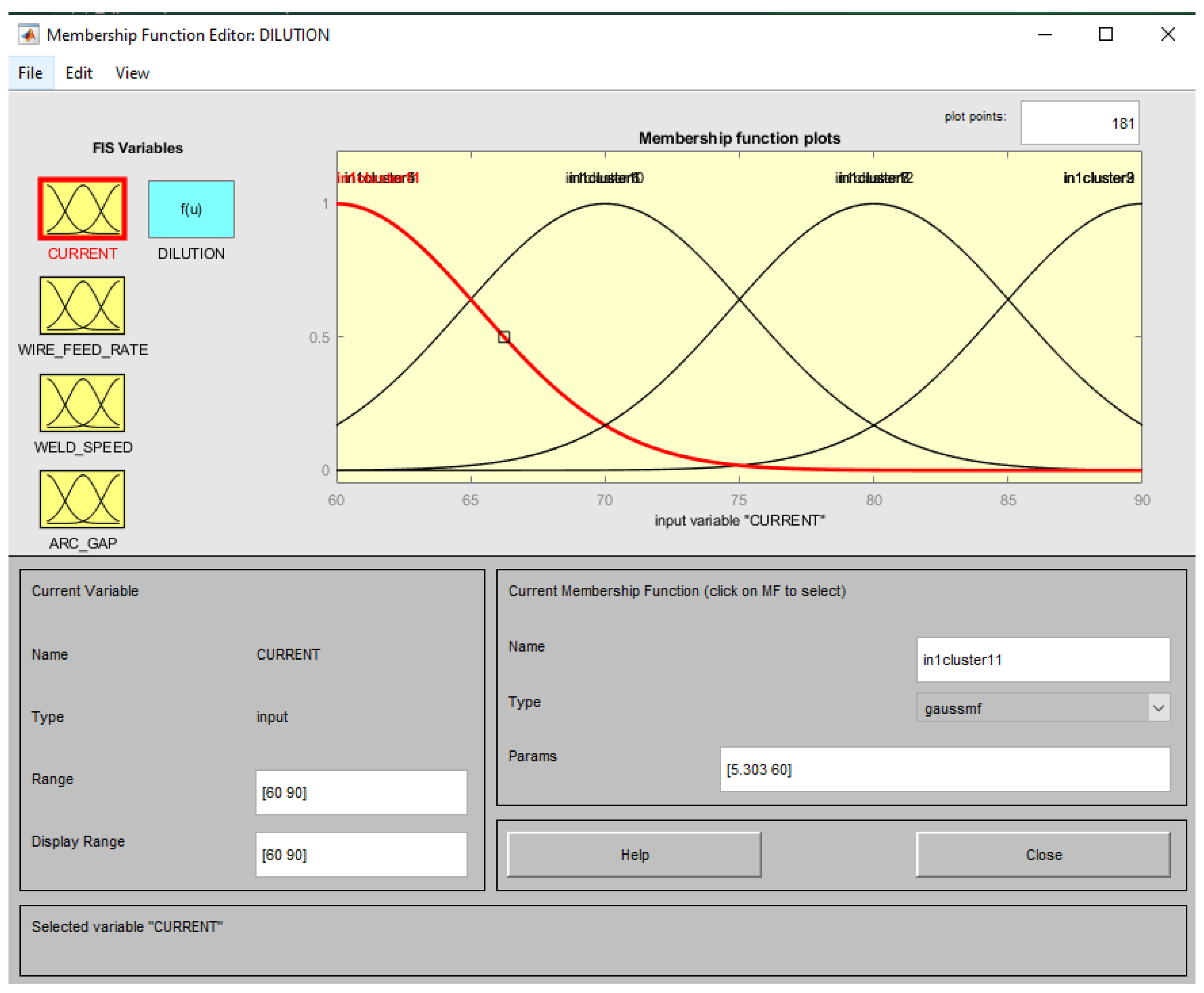
2.5.3. Adaptive Neuro-Fuzzy Inference System (ANFIS)

The ANFIS is a hybrid intelligent system possessing a multilayered feed-forward system with nodes. It is developed by an interconnection that integrates both training and logical thinking of neural networks and fuzzy logic. When compared to employing a single approach, ANFIS combines the learning skills of a neural network with the understanding capacities of fuzzy logic to provide better predictive accuracy. ANFIS uses input–output collections and a combination of IF–THEN fuzzy decision logic to provide a thinking approach of prediction models like a human brain. This heterogeneous network model possesses the potential to expand the predictive skills of ANFIS exceeding ANN and fuzzy inference system approaches [40]. ANFIS can determine the best range of membership functions by evaluating the translation correlation among the input and output values as well as using a back-propagation approach or in tandem with a regression model approach. This significantly decreases prediction error and increases flexibility to dynamic circumstances. This integrated system is basically considered to have two inputs (x & y) and one output (f) (Figure 5). A traditional framework for an initial level with two fuzzy if-then conditions, Sugeno-type fuzzy inference [23] system may be described as follows:

Condition 1: f₁ = p₁ + q₁ + r₁, if x = A₁ and y = B₁.

Condition 2: f₂ = p₂ + q₂ + r₂, if x = A₂ and y = B₂.

where p₁, p₂, q₁, q₂, r_1, and r₂ represent linear variables inside the following section, while A₁, A₂, B_1, and B₂ are nonlinear parameters.

The functionality of all layers in ANFIS is outlined as follows;

The first layer in the ANFIS layout is called the fuzzy layer. The modifiable elements were illustrated as squared nodes having x and y inputs and are labeled as A₁, A₂, B₁, and B₂ (Figure 5). A node in this layer represents a membership grade and has an adaptable local function (Equation (7)).

$$O_i^1={\mu }_{A_i}\left(x\right)$$

(7)

where $O_i^1$ represents output functions, ${\mu }_{A_i}$ represents relevant membership functions, and x refers to the input of the first node.

The second layer is named the product layer because the outcome of this layer is the products of the input, and each node is a static component (Equation (8)). The weighted factors of the subsequent layer are outputs W₁ and W₂.

$$O_i^2={\mu }_{A_i}\left(x\right).{\mu }_{B_i}\left(y\right),\mathrm{given}i=1,2$$

(8)

The third layer represents normalized mode and has fixed nodes (Equation (9)). By computing the relation of converting the ability of a single node to the total strengths, these can be normalized. The ratio of the ith firing value to the sum of all firing values was determined by:

$$O_i^3=\frac{{\omega }_i}{{\omega }_1+{\omega }_2}$$

(9)

The fourth layer is the defuzzification phase, which is denoted by rectangular vertices and has adaptable nodes (Equation (10)). The function of the node is determined by a nonfuzzy equation, which indicates the contributions of an ith rule to the total output.

$$O_i^4=O_i^3\left(\mathrm{pix}+\mathrm{qiy}+\mathrm{ri}\right)$$

(10)

The last layer essentially adds up all of the inputs to get the system calculated result (Equation (11)). The signaling node is a circular node defined by Σ,

$$O_i^4={{\displaystyle \sum }}_i{O}_i^3.f_i$$

(11)

In the current study, MATLABR2020 was utilized to create the ANFIS model. An ANFIS system, like ANNs, could be built using classification techniques to go beyond a given input to a certain desired output. Subtractive clustering is the approach used in the MATLAB ANFIS framework. Depending on the specific training set, there is considerable progress to be made to reach the convergence of the model.

3. Results and Discussion

3.1. Multiobjective Optimization—Statistical Model

The responses such as D%, R, P, and WB were obtained from the experimental run (

Table 3. Responses from experimental runs and grey relational analysis.

Sample No.	Experimental Results				Grey Coefficient				GRG	Rank
	D%	R	P	WB	D%	R	P	WB
DM-1	27.13	2.28	1.45	4.02	1.00	0.39	0.33	0.71	0.6095	9
DM-2	27.95	2.15	1.48	4.00	0.59	0.52	0.38	0.76	0.5616	11
DM-3	28.63	2.09	1.51	4.10	0.44	0.61	0.44	0.58	0.5179	12
DM-4	28.93	2.12	1.53	4.31	0.40	0.56	0.49	0.39	0.4590	16
DM-5	27.60	2.18	1.55	4.01	0.72	0.48	0.55	0.74	0.6207	5
DM-6	27.61	2.31	1.54	4.32	0.71	0.37	0.52	0.38	0.4954	14
DM-7	29.51	1.96	1.56	4.13	0.33	1.00	0.59	0.54	0.6158	8
DM-8 *	29.13	2.09	1.55	4.33	0.37	0.61	0.55	0.38	0.4780	15
DM-9	27.57	2.13	1.58	3.92	0.73	0.55	0.68	1.00	0.7392	2
DM-10	28.04	2.08	1.57	3.95	0.57	0.63	0.63	0.89	0.6800	3
DM-11	27.24	2.33	1.60	4.30	0.92	0.36	0.81	0.40	0.6196	6
DM-12	27.91	2.25	1.57	4.32	0.60	0.41	0.63	0.38	0.5081	13
DM-13	27.84	2.08	1.60	3.92	0.63	0.63	0.81	1.00	0.7667	1
DM-14	27.89	2.18	1.61	4.18	0.61	0.48	0.89	0.49	0.6194	7
DM-15	27.24	2.35	1.60	4.35	0.92	0.34	0.81	0.37	0.6093	10
DM-16	27.22	2.37	1.62	4.42	0.93	0.33	1.00	0.33	0.6491	4

* Initial design run (R, P & WB are in mm).

). For the context of this research, penetration should be increased, so larger-the-better formulations were utilized to determine optimal parameters. For D%, R, and BW, smaller-is-better conditions were employed as they need to be minimized. The wire feed rate and welding speed were determined to be the most important aspects affecting the outcomes, but other input variables also certainly contributed. The GRC and GRG of operations are tabulated in Table 3. The joint with specimen id DM-13 had the highest GRG value in the Taguchi L16 orthogonal array of 0.767.

As per the average table (

Table 4. Response table for average GRG.

Response Table
Level	L1	L2	L3	L4	diff	Optimal	Rank
Welding current	0.54	0.55	0.64	0.66	0.124	I4	2
Wire feed rate	0.68	0.59	0.59	0.52	0.160	F1	1
Welding speed	0.59	0.57	0.59	0.63	0.06	S4	3
CTWD	0.59	0.61	0.62	0.58	0.041	Z3	4
Optimal condition	Level
Based on Response table	I4F1S4Z3	Sample ID: C-1
Based on original L9	I4F1S4Z2	Sample ID: DM-13

), the optimal configuration of input variables for ideal results was I4F1S4Z3, which had welding current 90A, wire feed rate 3.1 m/min, welding speed 420 mm/min, and CTWD of 3 mm. However, the efficiency of the optimal input parameters can only be validated by a confirmation test. To improve overall weld efficiency, suitable input welding conditions have to be determined in order to achieve optimal weld bead. The welding current and welding speed significantly affected the bead width. If the welding speed was high, the time of electrode contacting the weld puddle was less and the amount of metal deposited on the weld pool per unit length decreased, thereby affecting the reinforcement and bead width. As the welding speed increased reinforcement and weld bead decreased. Similarly, increasing the wire feed rate increased the quantity of filler wire deposited to the weld zone, resulting in increased width and reinforcement. Figure 6 shows the micrographic images of obtained weld beads from the experimental runs.

In the case of penetration in the welded plates, welding current was the significant parameter. The penetration is directly proportional to welding current and we aimed to increase it in the current study. An increase in welding current and feed rate increased the heat input during the welding process. This increase in the heat input will cause the filler wire to deposit more molten metal inside the root gap and increase the penetration.

Determining GRG Using S/N Ratio

The average of all the levels of process variables was used to calculate the mean GRG. The GRG indicates the significance of the association between variables and the effectiveness of the input parameters. It demonstrates that I4F1S4Z3 was the best set of input parameters. The results of the grey-based Taguchi optimization were corroborated by these optimized values. From Figure 7, it is evident that the wire feed rate was the most important factor for determining GRG, accompanied by welding current and welding speed.

3.2. Regression Analysis

Linear regression models were postulated for all of these characteristics by taking into account all major and multiple interrelationships. For predicting and evaluating input variables, several scholars have been using multiple regression [41,42,43]. The data from the design of experiment in Table 1 and the responses in Table 3 were utilized to generate the formulas. The input parameters are symbolically represented before performing regression analysis (

Table 5. Notation for input parameters.

Input Parameters	Notation
Welding current	x(1)
Feed rate	x(2)
Welding speed	x(3)
CTWD	x(4)

).

The prediction model was developed using linear and quadratic regression equations to examine the relationship among the independent factors and their multiple responses. The regression model was developed using only the significant parameter within the 0.05 P-value. Based on the results from the least-square approach (R-Sq.) for all the output variables, a quadratic regression model was found to have higher R-Sq value than the linear model of the developed model (

Table 6. Developed linear regression equations for responses.

SI. No	Response	R-Sq (%)	Regression Equation
1	Dilution%	87.44	17.08 − 0.02616 *x(1) + 1.290 *x(2) + 0.02232 *x(3) − 0.0998 *x(4)
2	Reinforcement	91.2	3.439 + 0.003175 *x(1) + 0.0612 *x(2) − 0.004487 *x(3) + 0.01975 *x(4)
3	Penetration	90.2	1.022 + 0.003750 *x(1) + 0.0425 *x(2) + 0.000250 *x(3) + 0.00500 *x(4)
4	Bead Width	87.01	2.990 + 0.00255 *x(1) + 0.6200 *x(2) − 0.003000 *x(3) + 0.0170 *x(4)

and

Table 7. Quadratic regression equations for responses.

SI. No	Response	R-Sq (%)	Regression Equation
1	Dilution %	97.1	8.54 − 0.03363*x(1) + 1.290*x(2) + 0.04567*x(3) + 3.542*x(4) − 0.00934*x(3)*x(4)
2	Reinforcement	98.53	−71.4 + 0.2221*x(1) + 11.22*x(2) + 0.2637*x(3) − 3.28*x(4) − 0.001519*x(1)*x(1) − 0.000195*x(3)*x(3) + 0.0812*x(4)*x(4) − 0.0341*x(2)*x(3) + 0.850*x(2)*x(4)
3	Penetration	99.98	−1.451 + 0.06365*x(1) + 0.0645*x(2) + 0.001988*x(3) + 0.07569*x(4) − 0.000069*x(1)*x(1) + 0.000003*x(3)*x(3) − 0.003750*x(4)*x(4) − 0.004593*x(1)*x(2) − 0.000086*x(1)*x(3) − 0.000159*x(1)*x(4) + 0.000625*x(2)*x(3) − 0.000125*x(3)*x(4)
4	Bead Width	99.99	150.98 − 0.33441*x(1) − 23.148*x(2) − 0.5267*x(3) + 4.994*x(4) + 0.002562*x(1)*x(1) − 0.125*x(2)*x(2) + 0.000344*x(3)*x(3) − 0.115*x(4)*x(4) − 0.012316*x(1)*x(2) + 0.000047*x(1)*x(3) − 0.000909*x(1)*x(4) + 0.07375*x(2)*x(3) − 1.275*x(2)*x(4)

). Such regression models were then used to estimate weld bead shape characteristics and dilution percentage. The postulated equations for the bead geometry are:

Many researchers have used regression models for modeling and analyzing welding parameters [41,42,43,44]. It has been suggested that relative error should be less than 20% for statistical analysis to consider it to be reliable. Moreover, as wire feed rate and welding current were found to be most influential factors for multiobjective optimization in Section 3.1, additional levels of welding speed (420 mm/min) and welding current (100A) were used to determine the efficacy of the regression equation to predict other values outside L16 orthogonal array. Some additional experimental trials were therefore conducted and provided with a respective sample id (E) (

Table 8. Experimental runs outside the orthogonal array.

Sample No.	I	F	S	Z	D%	R	P	WB
C-1	90	3.1	420	3	27.47	2.06	1.61	3.78
E-1	100	3.1	420	2	27.71	2.13	1.61	4
E-2	100	3.3	400	1	28.23	2.15	1.62	4.24
E-3	100	3.5	380	4	27.19	2.41	1.67	4.58
E-4	100	3.7	360	3	26.49	2.5	1.66	4.5
E-5	90	3.9	360	3	26.49	2.45	1.67	4.38
E-6	90	3.1	440	3	28.60	2.01	1.58	3.98
E-7	90	3.1	420	5	28.68	2.06	1.55	4.09

).

From

Table 9. Tabulation of results obtained from developed prediction models within the input design range.

Sample No.	Regression Analysis				ANN				ANFIS
	D%	R	P	WB	D%	R	P	WB	D%	R	P	WB
DM-1	27.14	2.28	1.43	4.05	27.24	2.16	1.49	4.31	27.13	2.28	1.45	4.02
DM-2	28.12	2.15	1.46	4.04	27.94	2.14	1.49	4.00	27.95	2.15	1.48	4.00
DM-3	28.72	2.08	1.48	4.14	28.86	2.07	1.50	4.11	28.50	2.14	1.5	4.15
DM-4	28.95	2.10	1.50	4.35	28.93	2.12	1.49	4.31	28.93	2.12	1.53	4.31
DM-5	27.52	2.16	1.52	4.05	27.59	2.17	1.54	4.01	27.60	2.18	1.55	4.01
DM-6	27.60	2.28	1.52	4.35	27.61	2.30	1.55	4.30	27.61	2.31	1.54	4.32
DM-7	29.50	1.98	1.53	4.17	28.28	2.24	1.55	3.93	29.51	1.96	1.56	4.13
DM-8 *	28.84	2.08	1.52	4.37	27.71	2.32	1.53	4.28	28.20	1.88	1.49	3.94
DM-9	27.34	2.14	1.55	3.96	27.56	2.12	1.57	3.94	27.57	2.13	1.58	3.92
DM-10	28.15	2.07	1.54	3.99	28.04	2.07	1.58	3.94	28.04	2.08	1.57	3.95
DM-11	27.17	2.33	1.58	4.33	27.27	2.34	1.56	4.31	27.24	2.33	1.60	4.30
DM-12	27.97	2.21	1.54	4.36	27.33	2.33	1.55	4.28	28.70	2.45	1.68	4.52
DM-13	27.93	2.06	1.57	3.97	28.27	2.12	1.60	4.09	27.84	2.08	1.60	3.92
DM-14	27.84	2.19	1.58	4.22	27.89	2.18	1.61	4.19	27.89	2.18	1.61	4.18
DM-15	27.35	2.33	1.57	4.39	27.35	2.33	1.57	4.39	28.60	2.49	1.7	4.65
DM-16	27.27	2.36	1.59	4.45	27.43	2.35	1.54	4.38	27.22	2.37	1.62	4.42
Max. Error %	1.01	1.78	2.06	1.15	4.89	14.2	5.1	7.31	4.9	10	7	9
MRE	0.32	0.66	1.77	0.91	0.96	2.55	1.34	1.37	0.72	1.71	1.11	1.36
RMSE	0.12	0.02	0.03	0.04	0.51	0.1	0.03	0.1	0.53	0.09	0.05	0.15

* Initial design run.

, it can be observed that the regression equation can effectively predict the output response from the input parameters range used for the regression analysis well within 20%, whereas the prediction was dramatically reduced for test runs outside those input ranges. Table 9 also illustrates the results of the prediction model created from regression analysis and their performance by calculating mean relative error (MRE) and root mean square error (RMSE). As the regression model could not predict the responses outside the initial design effectively, this shows the need for machine learning artificial intelligence that can better understand the correlation between dependent and independent variables. The square root of the average variation of a dataset from the measured value to the predicted value is known as the root mean square error. The following equation gives the RMSE (Equation (12)):

$$\mathrm{RMSE}=\surd \left\{{{\displaystyle \sum }}_{i=0}^n\frac{{\left(predicted value-measured value\right)}^2}{n}\right\}$$

(12)

where n is the number of test results.

3.3. ANN Prediction Model

In the artificial neural configuration, the number of hidden layers and neurons are key aspects. Till now there has been no suitable technique for assessing such network aspects [45]. After many trial-and-error evaluations, the number of neurons in the hidden layer was set to 12 in this study since any higher number increased the computing time without reducing the overall percent error significantly. Furthermore, increasing the number of neurons to more than 12 had no influence on the outcomes. Moreover, when the number of hidden layers was increased to two, the findings were worse than when the layer was only one. Noted that the purpose of this research is to predict the weld bead characteristics of dissimilar joints, 75% of the test results were used as training data in the first network, and 25% were used to validate the trained network, i.e., a total of 12 out of 16 data sets were trained, with four data sets used for validation. This decision was premised on the reality that our training set was not noisy.

The network is trained for 1000 iterations to ensure that the network was well trained before testing and validation. Further training of the neural network seemed to have no influence on the prediction efficiency. The prediction efficacy of ANN was verified by the percentage of error obtained from the validation data and also by predicting from data sets outside the original L16 orthogonal inputs. The experimental runs performed outside the L16 array were given with sample id of E, before measuring the output characteristics. As shown in Figure 8, the regression coefficient of the network during training, testing and validation were 0.99998, 0.99927, and 1 respectively.

Table 9 shows the predicted outcomes from the feed-forward back-propagation neural network. The maximum relative error of projected values from the neural network was only 10%, so it is capable of predicting reasonably well. The responses predicted for the optimal parameter I4F1S4Z3 were found to be 28.47% of dilution, 2.09 mm of reinforcement, 1.58 mm of penetration, and 3.98 mm weld bead. The root mean square error of the ANN model was in the range of 0.07 to 0.63, which is far below the error range of the regression model.

3.4. The Adaptive Neuro-Fuzzy Inference System (ANFIS)

The available data set, which comprises 16 input data and their respective output data from the experiments conducted, was segregated into training and test sets to construct an ANFIS model for the welded dissimilar joint. The training set was assigned to 75% of the data set at arbitrary, whereas the other 25% was used to evaluate the efficacy of the network. The number of epochs was set to 1000 to assure that the learning process had adequate iterations. As illustrated in Figure 9, the fuzzy inference system had inputs that include welding current, feed rate, welding speed, and CTWD, whereas the output was the acquired dilution % or bead geometry generated by defuzzification. The Gaussian function was utilized as the membership function for the input variables. The Gaussian membership function was selected because the prediction error within the predicted and experimental data was the lowest of all the membership functions evaluated. The ANFIS model for the surface plot of the dilution % from proposed ANFIS is shown in Figure 10.

Figure 11 depicts the membership functions for dilution, which are made up of clustered linguistic variables. In comparison to grid partition, the subtractive clustering developing approach was more appropriate. The weighted average approach was used to defuzzify the data. Following that, the data were used to construct a hybrid algorithm that used the least square technique with the back-propagation conjugate gradient approach for training and improvement to determine the parameters of a Sugeno-type fuzzy system.

The predicted outcomes from the ANFIS model are compiled in Table 9. The prediction result of the ANFIS model was more accurate than ANN because it had a unique logic interface to understand the basic correlation between the dependent and independent variables. According to Table 9, the maximum relative errors of prediction for dilution, reinforcement, penetration, and bead width were 6%, 10%, 7%, and 9% respectively. The RMSE of the ANFIS model was in the range of 0.05 to 0.58, which is far lower than the ANN model.

Comparison between the Prediction Models

It is challenging to develop a predictive model that characterizes the relationship between process factors and weld bead properties because of their nonlinearity and uncertainties. This is the prime motive for using computational intelligence models (e.g., ANFIS and ANN) to create prediction models, but still both the predictive models should be compared to verify their efficiency of prediction.

The mean relative error percentage and root mean squared error data were used to evaluate the effectiveness of the two models. The relationship between experimentally observed and estimated weld bead shape and dilution percent predicted by ANN and ANFIS outside the input design is depicted in Figure 12.

The ANFIS is a hybrid intelligent system that combines artificial neural networks and fuzzy logic to effectively incorporate nonlinear effects in complicated processes. This is the fundamental reason that ANFIS has a higher prediction rate than ANN. The experimental results within the input design are compared to the predicted values in Table 9 and the variances are determined. It can be inferred from Table 9, that the prediction process performed by regression analysis was better with MRE in the range of 0.31–1.77 and RSME in the range of 0.02–0.12. Overall, the variance value (MRE and RMSE) indicates that the predicted rates appear to be effective. The performance of both the ANN and ANFIS model could be increased by utilizing data from additional trial runs.

The prediction of trail runs outside the L16 set was also better performed by the ANFIS model with less prediction error than the ANN model. According to this assessment (

Table 10. Tabulation of results obtained from developed prediction models outside input design range.

Sample No.	Regression Analysis				ANN				ANFIS
	D%	R	P	WB	D%	R	P	WB	D%	R	P	WB
C-1	27.55	1.82	1.56	4.35	28.47	2.09	1.58	3.98	27.9	2.08	1.6	3.93
E-1	27.60	1.39	1.57	5.29	27.96	2.16	1.61	4.19	28.00	2.09	1.61	3.94
E-2	27.51	1.52	1.59	5.52	27.84	2.18	1.61	4.25	28.00	2.19	1.62	4.2
E-3	27.02	1.66	1.58	5.62	27.37	2.34	1.55	4.40	28.8	2.51	1.72	4.68
E-4	26.93	1.70	1.61	5.66	27.54	2.35	1.55	4.42	27.4	2.39	1.63	4.45
E-5	27.52	2.66	1.57	3.96	27.34	2.35	1.50	4.40	27.2	2.37	1.62	4.42
E-6	27.90	1.63	1.52	4.39	29.03	2.00	1.55	3.96	29.2	2.18	1.67	4.1
E-7	26.79	1.83	1.51	4.43	28.27	2.02	1.56	3.96	29	2.24	1.66	4.13
Max. Error %	6.59	34.53	6.05	32.16	4.89	14.26	9.98	7.31	5.91	10.05	7.01	9.01
MRE	2.31	22.17	3.47	19.27	2.08	2.47	3.68	2.49	1.26	2.49	1.59	1.50
RMSE	0.86	0.55	0.06	0.90	0.65	0.07	0.08	0.13	0.77	0.11	0.06	0.09

), ANFIS appears to provide a slightly better response than the ANN for penetration and bead width as well as much better than regression analysis with RSME values of 0.06 and 0.09 respectively. For the prediction of dilution and reinforcement, ANN seems to provide better results with less RSME values of 0.65 and 0.07 respectively. This improvement is because of the fine experimental data used for the analysis.

The ANFIS is a hybrid intelligent system that combines artificial neural networks and fuzzy logic to effectively incorporate nonlinear effects in complicated processes. This is the fundamental reason that ANFIS has a higher prediction rate than ANN. During the design of ANN and ANFIS models, the selection of ANN parameters starts with a minimal number and gradually increased based on the performance of the tool. The objective of this task is to minimize the effect of overfitting. Yet it can be observed, for example, in predicting penetration by ANFIS.

3.5. Confirmatory Test

After the optimum parameters were identified from the grey-based Taguchi method, the final part of the study predicted and assessed the operational efficiencies of the outcomes. Confirmative testing was carried out based on the optimal parameters to verify the findings. The context of the overall study is determined from the relative error from the experimental trials. Moreover, the outcomes of the confirmation experiment appear to be in good agreement with the predicted outcomes (

Table 11. Confirmatory test results and GRG.

Response	Initial Design Run	ANN Model	ANFIS Model	Exp. Result	Improvement from Initial Condition (%)
Optimal parameters	DM8-I2F4S3Z2	C1-I4F1S4Z3	C1-I4F1S4Z3	C1-I4F1S4Z3
Dilution %	29.13	28.47	27.9	27.47	5.7
Reinforcement	2.09	2.09	2.08	2.06	1.4
Penetration	1.55	1.58	1.6	1.61	3.9
Bead Width	4.33	3.98	3.93	3.78	12.7
GRG	0.48	-	-	0.769	60.2

).

4. Conclusions

This study examines different optimization and prediction models for dilution and weld bead geometry of a dissimilar joint produced using stainless steel SS304 and mild steel AISI1008.

Multiobjective optimization of the input parameters of the GMAW process was performed using the grey-based Taguchi optimization method. The optimization search was implemented to design the decision space variables such as welding current, wire feed rate, welding speed, and CTWD for improving the dilution and weld bead geometry features, without sacrificing the mechanical properties. Further, the study identified that welding speed and welding current had an impact on bead width and reinforcement. Welding current was found to be the key influential factor of penetration in the weldment. The results obtained from the optimization model identified that the parametric optimal set is I4F1S4Z3 which denotes welding current 90 A, wire feed rate 3.1 m/min, welding speed 420 mm/min, and CTWD of 3 mm. Experimental analysis performed using these optimized parameters improved the performance of the welding process to an appreciable extent, for example, 5.7% was achieved for dilution and bead width improved by 12.7%.

Though regression analysis predicted effectively within the initial experimental design, the prediction failed tremendously for experiments outside it. Due to this lower prediction accuracy obtained from regression analysis outside the initial design range, machine learning models like ANN and ANFIS were used in this study. From the comparative study among machine learning models, it can be inferred that the predictions from the ANFIS model usually agreed well with the experimental data. The prediction performed outside the initial experimental design had minimum root mean square error of 0.06 and mean relative error of 1.79%, which are less than the ANN model that had minimum RSME and MRE in the range of 0.07 and 2.08% respectively.

The results exemplify that the ANFIS logic generated a slightly better prediction than the ANN for penetration and bead width. ANN model provided better prediction for dilution % and reinforcement, whereas both ANFIS and ANN performed much better than regression analysis outside the initial experimental design range. In this context, prediction from the ANFIS model is only considerably better than the ANN model, hence the research is inconclusive in determining which method is superior to the other.

It is worth mentioning that overfitting could be a limitation of the ANN and ANFIS models, the selection of ANN parameters should start with a minimal number and gradually increased with guidance of the ANN performance.

In the future, the study is planning to optimize mechanical properties associated with the welding process. This strategy will enhance the performance of the welded joint used in different manufacturing-oriented applications.

References

1. Teng, T.-L.; Fung, C.-P.; Chang, P.-H.; Yang, W.-C. Analysis of residual stresses and distortions in T-joint fillet welds. Int. J. Press. Vessel. Pip. 2001, 78, 523–538. [Google Scholar] [CrossRef]
2. Derakhshan, E.D.; Yazdian, N.; Craft, B.; Smith, S.; Kovacevic, R. Numerical simulation and experimental validation of residual stress and welding distortion induced by laser-based welding processes of thin structural steel plates in butt joint configuration. Opt. Laser Technol. 2018, 104, 170–182. [Google Scholar] [CrossRef]
3. Fuentes, A.L.G.; Salas, R.; Centeno, L.; del Rosario, A.V. Crack growth study of dissimilar steels (Stainless–Structural) butt-welded unions under cyclic loads. Procedia Eng. 2011, 10, 1917–1923. [Google Scholar] [CrossRef] [Green Version]
4. Devaraj, J.; Ziout, A.; Abu Qudeiri, J.E. Dissimilar Non-Ferrous Metal Welding: An Insight on Experimental and Numerical Analysis. Metals 2021, 11, 1486. [Google Scholar] [CrossRef]
5. Davis, J.R. (Ed.) Corrosion of Weldments; 1. print; ASM Internat: Materials Park, OH, USA, 2006; ISBN 978-0-87170-841-0. [Google Scholar]
6. Shushan, S.M.; Charles, E.A.; Congleton, J. The environment assisted cracking of diffusion bonded stainless to carbon steel joints in an aqueous chloride solution. Corros. Sci. 1996, 38, 673–686. [Google Scholar] [CrossRef]
7. Celik, A.; Alsaran, A. Mechanical and Structural Properties of Similar and Dissimilar Steel Joints. Mater. Charact. 1999, 43, 311–318. [Google Scholar] [CrossRef]
8. Ghosh, N.; Pal, P.K.; Nandi, G. GMAW dissimilar welding of AISI 409 ferritic stainless steel to AISI 316L austenitic stainless steel by using AISI 308 filler wire. Eng. Sci. Technol. Int. J. 2017, 20, 1334–1341. [Google Scholar] [CrossRef]
9. Ramarao, M.; King, M.F.L.; Sivakumar, A.; Manikandan, V.; Vijayakumar, M.; Subbiah, R. Optimizing GMAW parameters to achieve high impact strength of the dissimilar weld joints using Taguchi approach. Mater. Today Proc. 2021, in press. [Google Scholar] [CrossRef]
10. Dong, Q.; Shen, L.; Cao, F.; Jia, Y.; Liao, K.; Wang, M. Effect of Thermomechanical Processing on the Microstructure and Properties of a Cu-Fe-P Alloy. J. Mater. Eng. Perform. 2015, 24, 1531–1539. [Google Scholar] [CrossRef]
11. Rop, P. Drum Plus: A drum type HRSG with Benson benefits. Mod. Power Syst. 2010, 30, 35–40. [Google Scholar]
12. Dzierwa, P. Optimum heating of pressure components of steam boilers with regard to thermal stresses. J. Therm. Stresses 2016, 39, 874–886. [Google Scholar] [CrossRef]
13. ASME. Boiler and Pressure Vessel Code (BPVC) 2021 Complete Set; ASME: New York, NY, USA, 2021. [Google Scholar]
14. Rodrigues, D.M.; Menezes, L.F.; Loureiro, A.; Fernandes, J.V. Numerical study of the plastic behaviour in tension of welds in high strength steels. Int. J. Plast. 2004, 20, 1–18. [Google Scholar] [CrossRef] [Green Version]
15. Easterling, K. Introduction to the Physical Metallurgy of Welding; Elsevier Science: Kent, UK, 2014; ISBN 978-1-4831-4166-4. [Google Scholar]
16. Mohanty, U.K.; Sharma, A.; Abe, Y.; Fujimoto, T.; Nakatani, M.; Kitagawa, A.; Tanaka, M.; Suga, T. Geometric Model of the Weld Bead in DC and Square AC Submerged Arc Welding of 2.25 Cr-1 Mo Heat Resistant Steel. In Advances in Additive Manufacturing and Joining; Shunmugam, M.S., Kanthababu, M., Eds.; Lecture Notes on Multidisciplinary Industrial Engineering; Springer: Singapore, 2020; pp. 433–445. ISBN 978-981-329-432-5. [Google Scholar]
17. Zhao, L.; Shao, C.; Takashima, Y.; Minami, F.; Lu, F. Numerical Investigation on Fracture Initiation Properties of Interface Crack in Dissimilar Steel Welded Joints. Chin. J. Mech. Eng. 2020, 33, 27. [Google Scholar] [CrossRef] [Green Version]
18. Esme, U.; Bayramoglu, M.; Kazancoglu, Y.; Ozgun, S. Optimization of Weld Bead Geometry in TIG Welding Process using Grey Relation Analysis And Taguchi Method. Mater. Tehnol. 2009, 43, 143–149. [Google Scholar]
19. Jeyaganesh, D.; Ziout, A.; Qudeiri, J.A. Optimization of P-GMAW parameters using Grey relational analysis and Taguchi method. In Proceedings of the 2021 IEEE 12th International Conference on Mechanical and Intelligent Manufacturing Technologies (ICMIMT), Cape Town, South Africa, 13–15 May 2021; pp. 191–196. [Google Scholar]
20. Tomków, J.; Sobota, K.; Krajewski, S. Influence of tack welds distribution and welding sequence on the angular distortion of TIG welded joint. FU Mech. Eng. 2020, 18, 611–621. [Google Scholar] [CrossRef]
21. Vora, J.; Patel, V.K.; Srinivasan, S.; Chaudhari, R.; Pimenov, D.Y.; Giasin, K.; Sharma, S. Optimization of Activated Tungsten Inert Gas Welding Process Parameters Using Heat Transfer Search Algorithm: With Experimental Validation Using Case Studies. Metals 2021, 11, 981. [Google Scholar] [CrossRef]
22. Mastanaiah, P.; Sharma, A.; Reddy, G.M. Process parameters-weld bead geometry interactions and their influence on mechanical properties: A case of dissimilar aluminium alloy electron beam welds. Def. Technol. 2018, 14, 137–150. [Google Scholar] [CrossRef]
23. Nwobi-Okoye, C.C.; Ochieze, B.Q.; Okiy, S. Multi-objective optimization and modeling of age hardening process using ANN, ANFIS and genetic algorithm: Results from aluminum alloy A356/cow horn particulate composite. J. Mater. Res. Technol. 2019, 8, 3054–3075. [Google Scholar] [CrossRef]
24. Yuan, Z.; Wang, L.-N.; Ji, X. Prediction of concrete compressive strength: Research on hybrid models genetic based algorithms and ANFIS. Adv. Eng. Softw. 2014, 67, 156–163. [Google Scholar] [CrossRef]
25. Kochar, P.; Sharma, A.; Suga, T.; Tanaka, M. Prediction and Control of Asymmetric Bead Shape in Laser-Arc Hybrid Fillet-Lap Joints in Sheet Metal Welds. Lasers Manuf. Mater. Process. 2019, 6, 67–84. [Google Scholar] [CrossRef]
26. Tuominen, V. The measurement-aided welding cell—Giving sight to the blind. Int. J. Adv. Manuf. Technol. 2016, 86, 371–386. [Google Scholar] [CrossRef] [Green Version]
27. Xiong, J.; Zhang, G.; Hu, J.; Wu, L. Bead geometry prediction for robotic GMAW-based rapid manufacturing through a neural network and a second-order regression analysis. J. Intell. Manuf. 2014, 25, 157–163. [Google Scholar] [CrossRef]
28. Sreeraj, P.; Kannan, T.; Maji, S. Optimization of GMAW Process Parameters Using Particle Swarm Optimization. Int. Sch. Res. Not. Metall. 2013, 2013, 460651. [Google Scholar] [CrossRef] [Green Version]
29. Sreeraj, P.; Kannan, T.; Maji, S. Estimation of Optimum Dilution in the GMAW Process Using Integrated ANN-GA. J. Eng. 2013, 2013, 285030. [Google Scholar] [CrossRef] [Green Version]
30. Almeida, H.A.L.D.; Teixeira, F.R.; Mota, C.A.M.D.; Scotti, A. The Effect of Switchback Parameters on Root Pass Formation of Butt Welds with Variable Gap. J. Manuf. Mater. Process. 2019, 3, 54. [Google Scholar] [CrossRef] [Green Version]
31. Karadeniz, E.; Ozsarac, U.; Yildiz, C. The effect of process parameters on penetration in gas metal arc welding processes. Mater. Des. 2007, 28, 649–656. [Google Scholar] [CrossRef]
32. Casarini, A.; Coelho, J.P.; Olívio, É.; Braz-César, M.T.; Ribeiro, J. Optimization and Influence of GMAW Parameters for Weld Geometrical and Mechanical Properties Using the Taguchi Method and Variance Analysis. ICEUBI2019 Int. Congr. Eng. Eng. Evol. 2020, 5, 781–794. [Google Scholar] [CrossRef]
33. Kuo, C.-F.J.; Su, T.-L. Optimization of multiple quality characteristics for polyether ether ketone injection molding process. Fibers Polym. 2006, 7, 404–413. [Google Scholar] [CrossRef]
34. Kuo, Y.; Yang, T.; Huang, G.-W. The use of a grey-based Taguchi method for optimizing multi-response simulation problems. Eng. Optim. 2008, 40, 517–528. [Google Scholar] [CrossRef]
35. Liu, H.-T.; Cheng, H.S. An Improved Grey Quality Function Deployment Approach Using the Grey TRIZ Technique. Comput. Ind. Eng. 2016, 92, 57–71. [Google Scholar] [CrossRef]
36. Sharma, A.; Verma, D.K.; Arora, N. A scheme of comprehensive assessment of weld bead geometry. Int. J. Adv. Manuf. Technol. 2016, 82, 1507–1515. [Google Scholar] [CrossRef]
37. Choudhury, S.; Sharma, A.; Mohanty, U.K.; Kasai, R.; Komura, M.; Tanaka, M.; Suga, T. Mathematical model of complex weld penetration profile: A case of square AC waveform arc welding. J. Manuf. Process. 2017, 30, 483–491. [Google Scholar] [CrossRef]
38. Chaki, S. Neural networks based prediction modelling of hybrid laser beam welding process parameters with sensitivity analysis. SN Appl. Sci. 2019, 1, 1285. [Google Scholar] [CrossRef] [Green Version]
39. Choudhury, B.; Chandrasekaran, M.; Devarasiddappa, D. Development of ANN modelling for estimation of weld strength and integrated optimization for GTAW of Inconel 825 sheets used in aero engine components. J. Braz. Soc. Mech. Sci. Eng. 2020, 42, 308. [Google Scholar] [CrossRef]
40. Hosoz, M.; Ertunc, H.M.; Bulgurcu, H. An adaptive neuro-fuzzy inference system model for predicting the performance of a refrigeration system with a cooling tower. Expert Syst. Appl. 2011, 38, 14148–14155. [Google Scholar] [CrossRef]
41. Kim, J.; Kim, J.; Pyo, C.; Chun, K. Bead Geometry Prediction Model for 9% Nickel Laser Weldment, Part 1: Global Regression Model vs. Modified Regression Model. Processes 2021, 9, 793. [Google Scholar] [CrossRef]
42. Gunaraj, V.; Murugan, N. Application of response surface methodology for predicting weld bead quality in submerged arc welding of pipes. J. Mater. Process. Technol. 1999, 88, 266–275. [Google Scholar] [CrossRef]
43. Yang, L.J.; Bibby, M.J.; Chandel, R.S. Linear regression equations for modeling the submerged-arc welding process. J. Mater. Process. Technol. 1993, 39, 33–42. [Google Scholar] [CrossRef]
44. Vedrtnam, A.; Singh, G.; Kumar, A. Optimizing submerged arc welding using response surface methodology, regression analysis, and genetic algorithm. Def. Technol. 2018, 14, 204–212. [Google Scholar] [CrossRef]
45. Atuanya, C.U.; Government, M.R.; Nwobi-Okoye, C.C.; Onukwuli, O.D. Predicting the mechanical properties of date palm wood fibre-recycled low density polyethylene composite using artificial neural network. Int. J. Mech. Mater. Eng. 2014, 9, 7. [Google Scholar] [CrossRef] [Green Version]
Figure 1. Architecture of the current investigation.
Metals 11 01858 g001
Figure 2. Welding apparatus—1. weld machine with the controller; 2. self-build table CNC machine; 3. Z-axis coupled with weld torch; 4. personal computer.
Metals 11 01858 g002
Figure 3. Bead geometry, W—width; R—reinforcement; P—penetration; g—root gap.
Metals 11 01858 g003
Figure 4. Model of a classical artificial neural network.
Metals 11 01858 g004
Figure 5. Structural representation of ANFIS.
Metals 11 01858 g005
Figure 6. Macroscopic images of the weld bead: (a) sample DM7; (b) sample C1; (c) sample DM2 (d) sample DM9.
Metals 11 01858 g006
Figure 7. S/N ratio results for GRG.
Metals 11 01858 g007
Figure 8. ANN output prediction in training, testing, and validating phase versus experimental results.
Metals 11 01858 g008
Figure 9. Architecture of developed ANFIS model for predicting the output.
Metals 11 01858 g009
Figure 10. Surface plot of proposed ANFIS model for dilution.
Metals 11 01858 g010
Figure 11. Membership function for welding current on the Matlab interface.
Metals 11 01858 g011
Figure 12. Comparison between experimental and prediction models for runs outside the input experimental design.
Metals 11 01858 g012