Article

New Analyzing Approaches for In Situ Interdiffusion Experiments to Determine Concentration-Dependent Diffusion Coefficients in Liquid Al–Au

Institute for Materials Physics in Space, German Aerospace Center (DLR), 51170 Köln, Germany
*
Authors to whom correspondence should be addressed.
Metals 2021, 11(11), 1772; https://doi.org/10.3390/met11111772
Submission received: 1 October 2021 / Revised: 29 October 2021 / Accepted: 2 November 2021 / Published: 4 November 2021
(This article belongs to the Special Issue Thermodynamics and Kinetics in Metallurgical Processes)

Abstract

:
Interdiffusion coefficients are key parameters for the solidification process of liquid alloys. However, the determination of interdiffusion coefficients in liquid metals at high temperatures is a challenging and extensive task, due to a variety of potential systematic errors. In recent years we have developed an X-ray in situ shear cell method for the measurement of interdiffusion coefficients in binary metallic melts. This technique enables the monitoring of the experiment in order to exclude fatal errors. Utilizing X-ray contrast, the method also provides a time-resolved concentration distribution. Such an in situ data set contains significantly more information than ex situ evaluated experiments. Available analyzing strategies do not fully exploit this potential yet. We present three new analyzing approaches that are able to retrieve a concentration-dependent interdiffusion coefficient from only one in situ data set. In that way, larger concentration differences become accessible for an experiment, which considerably decreases efforts. Using simulations, the approaches are checked for robustness. Furthermore, the approaches are run on real in situ data from a binary (0 to 9 at% Au-content) Al–Au alloy at 1000 ° C which results in a concentration-dependent interdiffusion coefficient within the measured concentration range.

1. Introduction

Diffusion coefficients are key parameters for describing solidification processes in materials science. Especially in multi-component melts, interdiffusion (chemical diffusion) describes the transfer of atoms and thus the formation of the microstructure during solidification [1,2,3]. Predicting diffusion coefficients in metallic melts is not an easy task. There are different approaches in order to simulate diffusion processes in melts, e.g., molecular dynamics simulations [4,5,6,7] or mode coupling theory [8,9,10,11,12]. Even though the models have improved significantly in recent years, they are not yet sufficient to predict diffusion coefficients for a wide range of elements and with good accuracy. In order to be able to further develop models and at the same time to meet the requirements of materials science for precise diffusion coefficients, measurements of diffusion coefficients of high quality are indispensable.
While self-diffusion coefficients can be determined very precisely for most atoms with sufficient incoherent scattering cross-sections via QNS (quasielastic neutron scattering) [13,14], interdiffusion coefficients are primarily determined via the change of a concentration gradient over time [15,16,17]. To do this, we basically use a long cylindrical crucible/capillary in which two liquids of different concentrations are brought into contact. The diffusion then takes place over a certain period of time under constant thermal conditions. The concentration profile at a certain time c ( x , t end ) is then evaluated ex situ and a diffusion coefficient D is calculated using the known diffusion time t end . Occurring convection can strongly disturb these diffusion measurements since they lead to a change in concentration that takes place several orders of magnitude faster than it would be the case by diffusion itself. Experience has shown that convection can be reduced by using a thin capillary diameter and stable density layering [18,19]. A homogeneous and isothermal heat distribution and high thermal conductivity of the sample environment are also important in order to avoid density-driven convections in the sample medium.
Most interdiffusion experiments are based either on the long capillary method (LC) [20,21,22] or the shear cell method (SC) [23,24,25], which in various modifications represents the current state of the art. The measurement methods provide interdiffusion coefficients with an approximate accuracy of 20– 30 % for LC and 5– 15 % for SC [26,27], which makes it clear that interfering factors cannot be completely excluded. In order to be able to rule out density-driven convection, selected interdiffusion measurements are therefore carried out in space under microgravity conditions as reference [21,28].
Due to the lower susceptibility to failure, we specialized in shear cell technology and continuously developed it further. A shear cell consists of several segments with holes in which the sample material is located. After the samples have melted and the target temperature has been reached, the segments can be aligned so that the holes form a coherent capillary in which the diffusion experiment can take place. After a certain time, the segments are shifted again and the holes and the sample contents are separated, before the experiment is cooled down again. In that way, the concentration distribution at the start/end and the diffusion time are precisely known. However, shearing has the disadvantage that shear convection can occur due to the movement of the segments [29].
The solution to this problem was to combine shear cell technology with X-ray radiography in order to monitor the experiment, and exclude shear convection or bubbles in the capillaries as sources of error [19]. Since the concentration distribution in the capillary can also be measured in situ with a sufficiently high X-ray contrast of the sample, the shear cell was optimized for an X-ray imaging purpose [23]. The result was the compact high-temperature shear-cell furnace for in situ interdiffusion measurements [30].
An in situ interdiffusion experiment provides considerably more data than an ex situ experiment, as it contains a time-dependency of the concentration distribution c ( x , t ) . The evaluation method we have used so far, in this work called Common Erf-function Model, is a robust solution for an initial edge concentration function propagating with time. This method regards the data set as a multitude of ex situ measurements between the temporal start and endpoint of the measurement. Aside from that, it results in just one interdiffusion coefficient and only applies to small concentration differences in which the diffusion coefficient is not concentration dependent. At this point it should be mentioned that other analyzing methods have already been published, e.g., Boltzmann–Matano and Sauer–Freise Method [31,32]. However, these methods are originally designed for ex situ experiments, i.e., they are not specialized in time-resolved data sets. In addition, results show that these methods rely on a difference in the order of magnitude in the diffusion coefficient in order to deliver sufficiently good results. Such a large difference in the diffusion coefficient is seldom given in liquids, which is why the methods are primarily applied to solid–solid or solid–liquid diffusion experiments [33,34,35].
Within this work, we present novel evaluation methods to determine a concentration-dependent diffusion coefficient D ( c ) from just one in situ SC measurement data set c ( x , t ) . To do so, we first run the evaluation algorithms on noise-free simulated data sets to regain input parameters. In order to make a statement about robustness, we also use different degrees of synthetic noise on the simulated data sets. As a final demonstration of performance, the data set of an in situ Al–Au interdiffusion SC measurement is evaluated and compared with reference measurements from the same system. The Al–Au system was chosen because it has an excellent X-ray contrast and the results complement measurements of Al-based alloys that have been carried out in recent years [5,15,36,37,38,39].

2. Materials and Methods

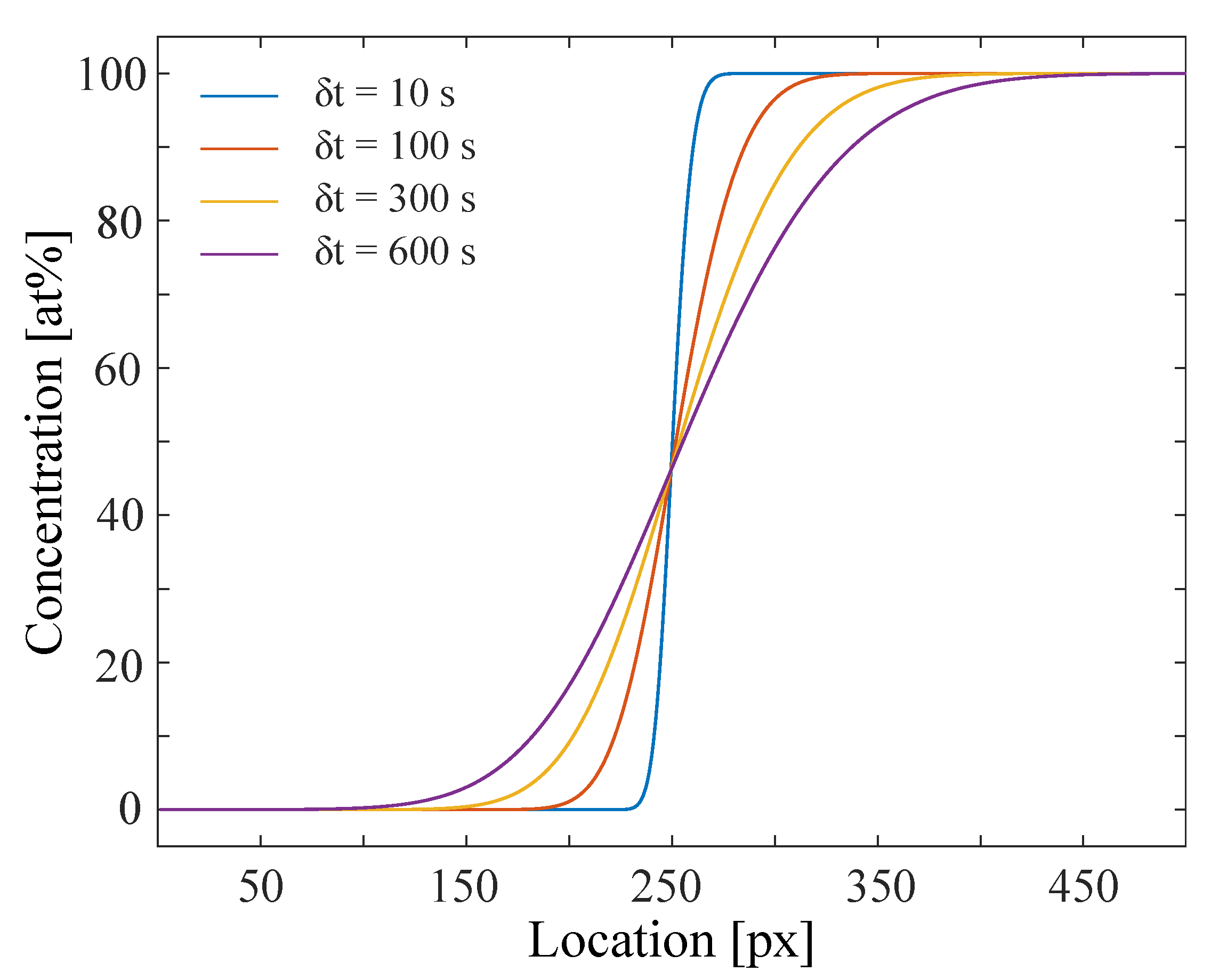
2.1. Simulation of Experiment-like Data Sets

In order to reproduce a data set, that is as identical as possible with the SC based experiments that we usually analyze [36], we choose comparable dimensions of resolution (50 µm/px) and range of the data points (500 px). The simulation starts with an edge function
c ( x , t 0 ) = c 1 for 0 < x 250 c 2 for 250 < x < 500
and evolves over time with different predefined sets of concentration dependent diffusion coefficients (Figure 1a). The simulation applies an finite differences approach, which in our case means that for a small time step (respective to the processes of millimeter scale we want to observe) of δ t = 10 3 s the changes in the concentration profile are calculated from one profile at time t 1 to the next at t 2 , following Fick’s 2nd Law (indeed, Fick’s 2nd Law is only valid for a constant D that is not position or concentration dependent. However, for later times and the used models the microscopic differences in concentration are sufficiently small to be neglected. Only close to the starting conditions (step function) this assumption is inaccurate. For a more accurate calculation see Chen et al. [40]).
c ( x , t 2 ) c ( x , t 1 ) = D ( c ) · Δ 2 c ( x , t 1 ) Δ x 2 · δ t .
The diffusion simulation is run until t end = 700 s. This is reasonable, as the simulation is only valid for profiles of infinite size. At 700 s the diffusion length is still smaller than the total range of the profile so the concentration at the boundary pixels does not change.
The time resolution of the data set we use for further analyzing is selected to be 1 s, so only every 1000th profile of the simulation is taken. The time resolution then matches the frame rate we have in our experiments. Further noise is added by a Gaussian noise operation. The simulation as described is realized in MATLAB. The simulated concentration profiles for different time steps are visualized in Figure 2.

2.2. Analyzing Models

2.2.1. Common Erf-Function Model

This approach is state of the art for ex situ diffusion experiments with concentration-independent D and is taken from Crank’s ‘The Mathematics of Diffusion’ [41]. The expression for an initial edge distribution of concentration c 1 and c 2 over time, is directly derived from Fick’s Law for the assumptions of a one-dimensional concentration gradient and a diffusion profile of infinite length (so edge effects are not taken into account):
c ( t , x ) = c 1 + c 2 2 + c 2 c 1 2 erf x x 0 4 D t
with x 0 being the center of the distribution. For the fitting procedure, c 1 and c 2 are constants, x 0 and D t are fitting parameters. From a linear behavior of D t ( t ) we can extract one (average) diffusion coefficient D for the concentration range between c 1 and c 2 . This approach is therefore only valid for a concentration difference, where D is concentration independent. In order to cover a large concentration range of D ( c ) many experiments need to be done.

2.2.2. Left/Right Erf-Function Model

Assuming that D does not change with concentration, it would be sufficient for the Erf-function Model to only fit one half of the concentration distribution, since in this case the distribution is mirror-symmetrical. However, if D changes with concentration, one-half of the distribution would be more elongated due to faster diffusion or more compressed due to slower diffusion compared to the other half. The effect of a concentration-dependent D ( c ) can be visualized by fitting the halves of the concentration distribution separately from each other. The distribution is split into halves at the previously determined x 0 position. The fitting is done with the same function as before (Equation (3)) but for the left side from 0 to x 0 and the right side from x 0 to 500 (px). The parameters c 1 , c 2 are again constant and x 0 and D t are fitting parameters. By that we obtain two diffusion coefficients from only one measurement.

2.2.3. Local Erf-Function Approach

If we pursue this idea, the next step is to fit an error function only locally. How large locally is, is defined by an algorithm coefficient Δ x . A larger Δ x will decrease the sensitivity of the fit but will also improve its noise robustness. The local fitting is done with the same function as for the Erf-function Model (Equation (3)) but for a data-range x ± Δ x at a given time t. From that we obtain an output data set of D t ( c , t ) , from which we can determine a concentration-dependent D ( c ) . The resolution of the concentration dependence of D ( c ) of course will scale with the accuracy of the values. The higher the resolution, the higher the error because we do less averaging.
Identifying the robustness of the models and applicability regarding noise is one of the aims of this work.

2.2.4. Numerical Fick’s Law Approach

The last model, which will provide the highest grade of resolution of the concentration dependency, is a numerical solution of Fick’s 2nd Law
d c ( x , t ) d t = D ( c ) · d 2 c ( x , t ) d x 2 .
From the simulation of an in situ measurement, we obtain a data set c ( x , t ) . Numerically we can therefore calculate the first derivative in time d c ( x , t ) d t and second derivative in space d 2 c ( x , t ) d x 2 . For this calculation a first-order polynomial is fitted in the time dimension and a second-order polynomial in the space dimension to any data point c ( x , t ) . As in the Local Erf-function Approach, there are algorithm coefficients Δ t and Δ x defining the fitting regime. From the polynomial coefficients the local derivatives are calculated. In that way we obtain several values for D ( c ) for the whole concentration range, that are used to calculate an average and standard deviation.
However experience from signal processing leads to the expectation, that noise multiplies heavily when calculating derivatives from a data set.

2.3. In Situ Shear-Cell Experiment

The experiments were performed using in situ SC technique as described in [30]. An extended version of the SC furnace has been used, with a larger capillary length of 26 mm, which increases the potential interdiffusion length and by that the total time for an experiment (up to δ t = 800 s). This is a beneficial enhancement of the prior furnace, as we can access a longer time period to observe the diffusion process while excluding potential systematic errors at the beginning or end of a measurement. At the beginning, shear convection rolls from the shearing process at δ t = 0 can occur. These lead to a faster local mixing, to deformations of the original step function and therefore to systematic errors in the analysis. The prior presented analyzing approaches are more sensitive to local disturbances of the concentration profile. The further the profile propagates in time, the more these deformations smooth out. Additionally, at the end of a measurement δ t > 800 s there come edge effects of the capillary into play, which thwart the diffusion process. That is why it is reasonable to access an analyzing regime of 200 s < δ t < 600 s in order to avoid systematic errors.
The concentrations of the two parts of the interdiffusion couple were chosen to be 0 and 9 at% Au in Al at 1000 ° C (hereinafter the form 0/9 at% Au–Al is used to describe the concentration step of an interdiffusion experiment). The choice weighs the width of the concentration range against excessively high melting temperatures. As we do not have an initial D ( c ) as for the simulated data to compare, we also measured data sets for smaller concentration differences (0/3, 3/6, and 6/9 at% Au–Al) as reference. They were alloyed from high-grade pure elements (Au wire, 2.0 mm, 99.9985 % by Alfa Aesar; Al shot, 4–8 mm, 99.999 % by Alfa Aesar) in an arc melter under purified Argon atmosphere. For X-ray imaging we use a micro-focus X-ray source (XT9160-TED, Viscom AG, Hannover, Germany) which was operated at 150 kV and 250 µA and a (2 mm) CdTe detector with a 100 µm pixel size (XC-Thor series, Direct Conversion AB, Danderyd, Sweden). The effective pixel size for the experiment was ∼50 µm.

3. Results

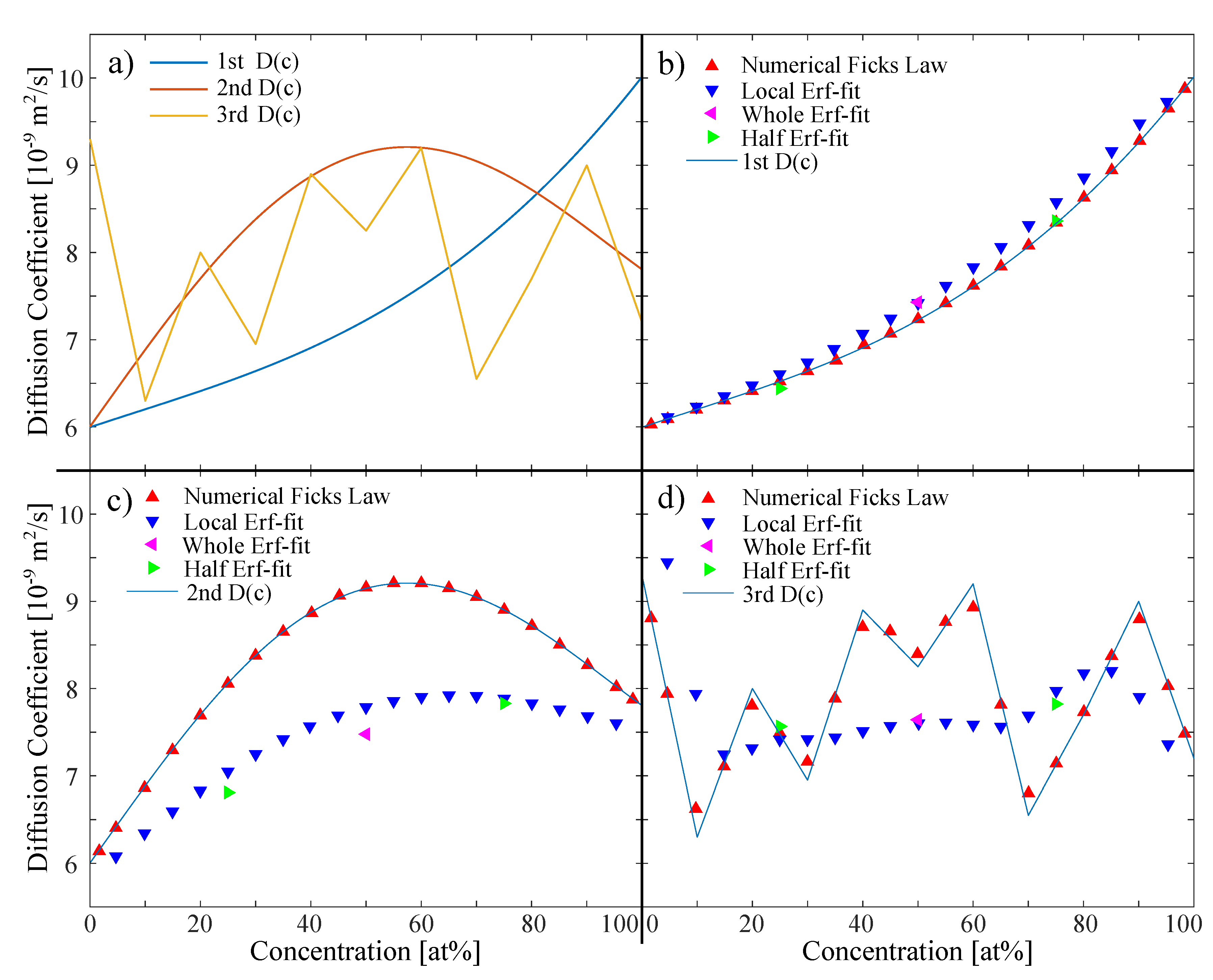
3.1. Noiseless Simulated In Situ Data

In order to model different concentration-dependent diffusion coefficients, we chose three different D ( c ) as input coefficients for the simulation (Figure 1a), to show the robustness and sensitivity of the four analyzing approaches. The diffusion coefficients are selected in an order of magnitude (5 to 10 × 10 9 m 2 /s) which corresponds to most metallic melts [15,36,37,38].
The 1st  D ( c ) is a diffusion coefficient exemplary for a steadily increasing/decreasing concentration dependence, which is for example observed in liquid Al–Ag [38]. The 2nd D ( c ) has a local maximum at ≈60 at%, which was found for example in simulations of Al–Ni melts [11]. The 2nd D ( c ) is exemplary for a diffusion coefficient with a local minimum/maximum at a certain concentration. The 3rd D ( c ) one is a random distribution, that we use to show the sensitivity of the analyzing approaches and will only be presented in the evaluation of the noiseless data set.
The 1st D ( c ) shows a steady increase in the diffusion coefficient. All models are able to recover the input coefficients or at least a local average of them. For all approaches using an Erf-fit, a systematic error arises within the center concentration range, where the fitting results appear a little larger than the input coefficients. The Numerical Fick’s Law Approach shows the best recovery of the input coefficients for zero noise conditions as can be seen in Figure 1b.
For the 2nd D ( c ) with a local maximum, there is a more severe systematic error for the analyzing approaches using an Erf-fit. Diffusion coefficients at center concentrations seem to be underrepresented compared to those at the sides. In this case, the recovered diffusion coefficients are much lower than the input D ( c ) . The Numerical Fick’s Law Approach recovers the input coefficients very well as shown in Figure 1c.
For the random-like 3rd D ( c ) distribution of the input coefficient (Figure 1d), the whole and left/right Erf-fit do not have any informative value, except some kind of total average. The local Erf-fit approach shows at least a low sensitivity at the sides but with a large systematic error. As for the previous D ( c ) , the Erf-fit show the highest systematic error within the center concentration range.
Still, the Numerical Fick’s Law Approach shows a high sensitivity at any concentration and reproduces the random-like input coefficient quite well, even though for some coefficients, a small offset is visible.

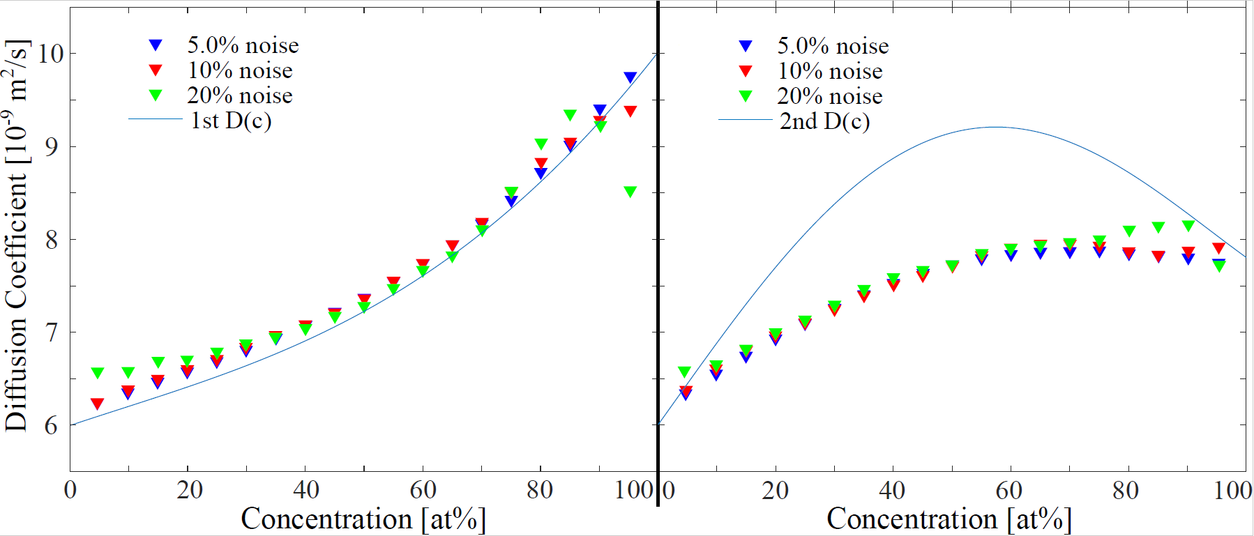
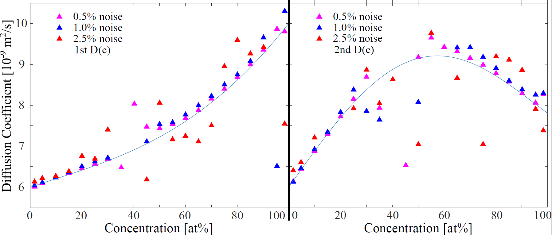
3.2. Robustness against Noise

In this section, we investigate the robustness of the Local Erf-Fit Model and the Numerical Fick’s Law Approach against noise. In order to improve noise stability of the fits the algorithm coefficients are set to Δ x = 25 px and Δ t = 25 s, which showed the best compromise between sensitivity and noise susceptibility during testing cycles. Indeed, the quantification of best compromise between sensitivity and noise susceptibility is a challenging task. On basis of the noise-free concentration profiles of 2nd D ( c ) we determined a maximum Δ x and Δ t for the Numerical Fick’s Law Approach that only lead to 1 % difference to the input 2nd D ( c ) . In that way we covered “best” sensitivity for our system. For other systems these values can have a different optimum. That is why we suggest running the algorithm on different Δ x and Δ t in order to clarify their impact on the results.
The approaches using the whole Erf-fit and Left/Right Erf-fit are not further investigated regarding noise, as they show a high robustness up to 40 % of noise. The systematic error for these two models turns out to be stable even for high noise.

3.2.1. Noise on Local Erf-Fit

The Local Erf-fit Approach shows a high robustness against noise (Figure 3). Interestingly the previously observed systematic error seems not to be noise dependent. For both input models of D ( c ) , the center of the concentration distribution stays stable, even for high noise conditions of 20 % . However, for high noise disturbance > 10 % the results close to the side concentrations c 1 and c 2 involve an offset to the input coefficients. Remarkable is that even for high noise conditions the calculated coefficients do not scatter randomly.

3.2.2. Noise on Numerical Fick’s Law Approach

The results in Figure 4 show, that the Numerical Fick’s Law Approach shows a high susceptibility to noise. If the statistical noise is larger than 1.0 % in the simulated data set, the results from the analyzing approach are scattering too much to make qualitatively correct statements about them. The error of results (even though not plotted in the graph) is heavily increasing with noise as well. The errorbars for the scattering data points lie outside the chosen scale of the plots.
The center of the concentration distribution at 50 at % and the sides close to c 1 and c 2 , show a significantly higher susceptibility to noise compared to the concentration ranges in between.
The high sensitivity of the model becomes its weakness for noisy conditions. This can directly be related to the calculation of local derivatives, that are highly sensitive to noise.

3.3. Performance on Experimental Data Sets of Al–Au System

Figure 5 shows the experimentally determined concentration profiles after background correction procedures. Compared to the simulated concentration profiles of Figure 2, we have a statistic noise of ∼2.0%. Aside from that, there are slight deformations of the profiles, either due to shear convection in the early period of the experiment or over-correction during the post-processing of the data. For the analysis we use a δ t of 200 to 600 s, where these deformations already have dissolved.
Figure 6 shows the results of the different analyzing approaches on the Al–Au SC data sets. The whole/half results show good agreement with the reference measurement. The left/right arms of the half Erf-fit approach also show a decrease of the diffusion coefficient with increasing Au-content in the Al-melt.
The next step further in resolving the concentration dependence of the diffusion coefficient is the local Erf-fit approach. Close to the boundary concentrations (0 and 9 at% Au-content) the diffusion coefficients start to scatter heavily, which is why they were excluded here. This effect had already been observed for the simulated data (Figure 3). The reason for that can be found in the poor fitting potential on the flat shoulders of the concentration profile. Close to the center concentration (4.5 at %Au-content) the results follow the reference measurement very well. The error of the local Erf-fit approach diffusion coefficients lies between 5 and 10%.
The highest resolution in concentration dependence can be obtained by the Numerical Fick’s Law Approach. The weakness of this approach is the center concentration regime (left out in Figure 6), as d 2 c / d x 2 is close to zero here. We already observed this in the simulated data (Figure 4), where the center concentration diffusion coefficients begin to scatter with higher noise ratios. Interestingly the Numerical Fick’s Law Approach is more stable towards the end concentrations than the local Erf-fit approach. Although the calculated error bars from the analysis are very large (∼40%), the average diffusion coefficients of adjacent concentrations do not scatter much, which still gives a good estimation for the actual diffusion coefficient within this concentration regime. The course at the low concentrations ∼2.5 at% Au-content even suggests a local maximum, but this observation is very vague because of the small increase and the large error.
In combination, the three approaches allow an estimation of the concentration dependence of the diffusion coefficient for a large concentration range. From only one measurement we can assume that the diffusion coefficient follows a black dotted line which represents an average of the obtained results from the analyzing algorithms with an accuracy of ∼15%.
If we compare the results of the Al–Au system with other Al–Ni/Cu/Ag results from the last years, we have the following to remark: Since the other systems were measured at lower temperatures between 700 and 900 ° C, they can not be compared in absolute values. However, the concentration dependence can be evaluated. The diffusion coefficient changes little for the Al–Ni system with concentration, while the diffusion coefficient within the Al-Cu/Ag/Au group decreases with a larger minority concentration. The decrease even seems to be stronger depending on the nuclear size or weight of the atoms, see Al–Au (at 1000 ° C; 0 to 9 at% Au: 12 to 8 × 10 9 m 2 /s) and decreases further for Al–Ag (710 ° C: 2 to 20 at% Ag: 8 to 4 × 10 9 m 2 /s) [38] and Al–Cu (700 ° C: 2 to 20 at% Cu: 5 to 3 × 10 9 m 2 /s) [15]. Interestingly, the interdiffusion for small amounts of minority atoms seems to be faster the heavier/larger they are. In order to be able to make more precise statements about these observations, comparative measurements of the systems at the same temperature would be useful. In addition, a measurement of self-diffusion coefficients is suggested to see if the mobility of both elements increases equally or if one of the two specimens is more likely to be affected by concentration changes.

4. Conclusions

The starting point of this work was to find new analyzing techniques specialized in in situ SC interdiffusion data, that yield a concentration-dependent diffusion coefficient from only one measurement. Making use of the time-resolved information will unlock new experimental strategies, e.g., performing measurements on larger concentration differences that until now had to be performed in smaller concentration steps. By that the experimental effort is directly decreased.
We present three new analyzing techniques, namely Left/Right Erf-function Model, Local Erf-function Approach, and the Numerical Fick’s Law Approach. We use these approaches on simulated experiment-like data to find the strengths and weaknesses of the approaches before testing them on real measurement data.
The Left/Right Erf-function Model is robust against noise and comes with the smallest error. However, it only covers a small concentration range and is inaccurate when the diffusion coefficient changes strongly within the boundary concentrations of the experiment. The Local Erf-function Approach covers the whole concentration range of the experiment, but is weak close to the boundary concentrations. The weakness increases with noise ratio. Still, it is less noise susceptible than the Numerical Fick’s law approach, but comes with a larger error than the Left/Right Erf-function Model. It is also inaccurate if the diffusion coefficient has a local minimum/maximum within the boundary concentrations. The last approach, the numerical solution of Fick’s Law, works better at boundary concentrations but is weak at the center concentrations. It has the largest noise susceptibility and comes with the largest error but delivers the most accurate reconstruction of the diffusion coefficient for almost ideal noiseless data-sets (noise < 1.5%).
The approaches were also used to analyze real in situ SC data from an Al-0/9 at% Au experiment. The X-ray absorption contrast is very good for this alloy system and the statistic noise is ∼2.0%. All approaches were applied to the data with a focus on the strengths of each approach. As a result we estimated a concentration-dependent diffusion coefficient over the whole concentration range with an approximated error of ∼15%. This is a proof of concept, which can be applied even to higher concentration differences. Key criteria for application are a good contrast and a low noise ratio of <2.0%.

Author Contributions

Conceptualization, A.M., E.S. and T.S.; methodology, T.S.; software, T.S.; investigation, T.S.; writing—original draft preparation, T.S.; writing—review and editing, A.M. and E.S.; supervision, A.M. All authors have read and agreed to the published version of the manuscript.

Funding

This research received no external funding.

Institutional Review Board Statement

Not applicable.

Informed Consent Statement

Not applicable.

Data Availability Statement

The measured data and the programmed analyzing tools (MATLAB scripts) can be provided by the author on request.

Acknowledgments

The authors would like to thank C. Dreißigacker and D. Bräuer for technical support with the experimental setup and the workshop department for advice and assistance in manufacturing the shear cell components.

Conflicts of Interest

The authors declared no conflict of interest.

References

  1. Symeonidis, K.; Apelian, D.; Makhlouf, M. Controlled diffusion solidification: Application to metal casting. Metall. Sci. Technol. 2008, 26, 39–44. [Google Scholar]
  2. Miller, J.; Yuan, L.; Lee, P.; Pollock, T. Simulation of diffusion-limited lateral growth of dendrites during solidification via liquid metal cooling. Acta Mater. 2014, 69, 47–59. [Google Scholar] [CrossRef]
  3. Becker, M.; Klein, S.; Kargl, F. Free dendritic tip growth velocities measured in Al-Ge. Phys. Rev. Mater. 2018, 2, 073405. [Google Scholar] [CrossRef] [Green Version]
  4. Kresse, G.; Hafner, J. Ab initio molecular dynamics for liquid metals. Phys. Rev. B 1993, 47, 558. [Google Scholar] [CrossRef]
  5. Horbach, J.; Das, S.K.; Griesche, A.; Macht, M.P.; Frohberg, G.; Meyer, A. Self-diffusion and interdiffusion in Al 80 Ni 20 melts: Simulation and experiment. Phys. Rev. B 2007, 75, 174304. [Google Scholar] [CrossRef] [Green Version]
  6. Horbach, J.; Rozas, R.; Unruh, T.; Meyer, A. Improvement of computer simulation models for metallic melts via quasielastic neutron scattering: A case study of liquid titanium. Phys. Rev. B 2009, 80, 212203. [Google Scholar] [CrossRef]
  7. Han, X.; Schober, H. Transport properties and Stokes-Einstein relation in a computer-simulated glass-forming Cu33.3Zr66.7 melt. Phys. Rev. B 2011, 83, 224201. [Google Scholar] [CrossRef] [Green Version]
  8. Zöllmer, V.; Rätzke, K.; Faupel, F.; Meyer, A. Diffusion in a metallic melt at the critical temperature of mode coupling theory. Phys. Rev. Lett. 2003, 90, 195502. [Google Scholar] [CrossRef] [Green Version]
  9. Voigtmann, T.; Meyer, A.; Holland-Moritz, D.; Stüber, S.; Hansen, T.; Unruh, T. Atomic diffusion mechanisms in a binary metallic melt. EPL Europhys. Lett. 2008, 82, 66001. [Google Scholar] [CrossRef]
  10. Gotze, W. Complex dynamics of glass-forming liquids. Phys. J. 2009, 8, 52. [Google Scholar]
  11. Kuhn, P.; Horbach, J.; Kargl, F.; Meyer, A.; Voigtmann, T. Diffusion and interdiffusion in binary metallic melts. Phys. Rev. B 2014, 90, 024309. [Google Scholar] [CrossRef] [Green Version]
  12. Nowak, B.; Holland-Moritz, D.; Yang, F.; Voigtmann, T.; Kordel, T.; Hansen, T.; Meyer, A. Partial structure factors reveal atomic dynamics in metallic alloy melts. Phys. Rev. Mater. 2017, 1, 025603. [Google Scholar] [CrossRef]
  13. Meyer, A. Self-diffusion in liquid copper as seen by quasielastic neutron scattering. Phys. Rev. B 2010, 81, 012102. [Google Scholar] [CrossRef]
  14. Kargl, F.; Weis, H.; Unruh, T.; Meyer, A. Self diffusion in liquid aluminium. J. Phys. Conf. Ser. 2012, 340, 012077. [Google Scholar] [CrossRef]
  15. Sondermann, E.; Jakse, N.; Binder, K.; Mielke, A.; Heuskin, D.; Kargl, F.; Meyer, A. Concentration dependence of interdiffusion in aluminum-rich Al-Cu melts. Phys. Rev. B 2019, 99, 024204. [Google Scholar] [CrossRef]
  16. Belova, I.V.; Heuskin, D.; Sondermann, E.; Ignatzi, B.; Kargl, F.; Murch, G.E.; Meyer, A. Combined interdiffusion and self-diffusion analysis in Al-Cu liquid diffusion couple. Scr. Mater. 2018, 143, 40–43. [Google Scholar] [CrossRef]
  17. Griesche, A.; Macht, M.P.; Frohberg, G. First results from diffusion measurements in liquid multicomponent Al-based alloys. J. Non-Cryst. Solids 2007, 353, 3305–3309. [Google Scholar] [CrossRef]
  18. Suzuki, S.; Kraatz, K.H.; Frohberg, G. Reduction of convection in diffusion measurement using the shear cell by stabilization of density layering on the ground. J. Jpn. Soc. Microgravity Appl. 2011, 28, 100. [Google Scholar]
  19. Kargl, F.; Sondermann, E.; Weis, H.; Meyer, A. Impact of convective flow on long-capillary chemical diffusion studies of liquid binary alloys. High Temp. Press. 2013, 42, 3–21. [Google Scholar]
  20. Griesche, A.; Zhang, B.; Solórzano, E.; Garcia-Moreno, F. Note: X-ray radiography for measuring chemical diffusion in metallic melts. Rev. Sci. Instrum. 2010, 81, 056104. [Google Scholar] [CrossRef] [PubMed]
  21. Meyer, A.; Kargl, F. Diffusion of Mass in Liquid Metals and Alloys-Recent Experimental Developments and New Perspectives. Int. J. Microgravity Sci. Appl. 2013, 30, 30. [Google Scholar]
  22. Weis, H.; Kargl, F.; Kolbe, M.; Koza, M.; Unruh, T.; Meyer, A. Self-and interdiffusion in dilute liquid germanium-based alloys. J. Phys. Condens. Matter 2019, 31, 455101. [Google Scholar] [CrossRef]
  23. Neumann, C.; Sondermann, E.; Kargl, F.; Meyer, A. Compact high-temperature shear-cell furnace for in-situ diffusion measurements. J. Phys. Conf. Ser. 2011, 327, 012052. [Google Scholar] [CrossRef] [Green Version]
  24. Geng, Y.; Zhu, C.; Zhang, B. A sliding cell technique for diffusion measurements in liquid metals. AIP Adv. 2014, 4, 037102. [Google Scholar] [CrossRef]
  25. Zhong, L.; Hu, J.; Geng, Y.; Zhu, C.; Zhang, B. A multi-slice sliding cell technique for diffusion measurements in liquid metals. Rev. Sci. Instrum. 2017, 88, 093905. [Google Scholar] [CrossRef] [PubMed]
  26. Griesche, A.; Macht, M.; Frohberg, G. Diffusion in Metallic Melts. Defect Diffus. Forum 2007, 266, 101–108. [Google Scholar] [CrossRef]
  27. Griesche, A.; Zhang, B.; Horbach, J.; Meyer, A. Interdiffusion and Thermodynamic Forces in Binary Liquid Alloys. Mater. Sci. Forum 2010, 649, 481–486. [Google Scholar] [CrossRef]
  28. Masaki, T.; Fukazawa, T.; Matsumoto, S.; Itami, T.; Yoda, S. Measurements of diffusion coefficients of metallic melt under microgravity—Current status of the development of shear cell technique towards JEM on ISS. Meas. Sci. Technol. 2005, 16, 327. [Google Scholar] [CrossRef]
  29. Griesche, A.; Kraatz, K.H.; Frohberg, G.; Mathiak, G.; Willnecker, R. Liquid diffusion measurements with the shear cell technique-study of shear convection. Microgravity Res. Apl. Phys. Sci. Biotechnol. 2001, 454, 497. [Google Scholar]
  30. Sondermann, E.; Neumann, C.; Kargl, F.; Meyer, A. Compact high-temperature shear-cell furnace for in-situ interdiffusion measurements. High Temp. Press. 2013, 42, 012052. [Google Scholar]
  31. Ahmed, T.; Belova, I.; Evteev, A.; Levchenko, E.; Murch, G. Comparison of the Sauer-Freise and Hall methods for obtaining interdiffusion coefficients in binary alloys. J. Phase Equilibria Diffus. 2015, 36, 366–374. [Google Scholar] [CrossRef]
  32. Olaye, O.; Ojo, O. A New Analytical Method for Computing Concentration-Dependent Interdiffusion Coefficient in Binary Systems with Pre-existing Solute Concentration Gradient. J. Phase Equilibria Diffus. 2021, 42, 303–314. [Google Scholar] [CrossRef]
  33. Zhang, Q.; Zhao, J.C. Extracting interdiffusion coefficients from binary diffusion couples using traditional methods and a forward-simulation method. Intermetallics 2013, 34, 132–141. [Google Scholar] [CrossRef]
  34. Wierzba, B.; Skibiński, W. The generalization of the Boltzmann–Matano method. Phys. A Stat. Mech. Appl. 2013, 392, 4316–4324. [Google Scholar] [CrossRef]
  35. Olaye, O.; Ojo, O. Time variation of concentration-dependent interdiffusion coefficient obtained by numerical simulation analysis. Materialia 2021, 16, 101056. [Google Scholar] [CrossRef]
  36. Sondermann, E.; Kargl, F.; Meyer, A. Influence of cross correlations on interdiffusion in Al-rich Al-Ni melts. Phys. Rev. B 2016, 93, 184201. [Google Scholar] [CrossRef] [Green Version]
  37. Lee, N.; Cahoon, J. Interdiffusion of copper and iron in liquid aluminum. J. Phase Equilibria Diffus. 2011, 32, 226–234. [Google Scholar] [CrossRef]
  38. Engelhardt, M.; Meyer, A.; Yang, F.; Simeoni, G.; Kargl, F. Self and chemical diffusion in liquid Al-Ag. Defect Diffus. Forum 2016, 367, 157–166. [Google Scholar] [CrossRef] [Green Version]
  39. Zhang, B.; Griesche, A.; Meyer, A. Diffusion in Al-Cu melts studied by time-resolved X-ray radiography. Phys. Rev. Lett. 2010, 104, 035902. [Google Scholar] [CrossRef]
  40. Chen, W.; Li, Q.; Zhang, L. A novel approach to eliminate the effect of external stress on interdiffusivity measurement. Materials 2017, 10, 961. [Google Scholar] [CrossRef] [Green Version]
  41. Crank, J. The Mathematics of Diffusion; Clarendon Press: Oxford, UK, 1975. [Google Scholar]
Figure 1. (a) Three concentration dependent diffusion coefficients D ( c ) used as input for the simulation of the concentration profiles: 1st steadily increasing, 2nd with a local maximum, and 3rd completely random distribution. The order of magnitude was chosen to match other binary melts. (bd) Comparison of results for the analysis of the noise-free simulated data-sets. Local Erf-fit and Numerical Fick’s Law Approach are run on Δ x = 5 px and Δ t = 5 s.
Metals 11 01772 g001
Figure 2. Interdiffusion simulation of a concentration profile starting from a step function of maximum concentration difference (0 and 100 at% of specimen B in A) propagating with time. The diffusion coefficient D ( c ) ranges from 6 to 10 [ × 10 9 m 2 /s] (referred to 1st D ( c ) of Figure 1).
Metals 11 01772 g002
Figure 3. Effect of noise on the Local Erf-fit analyzing approach. Error bars exceed the chosen scale of the graph. They have not been plotted in favor of a clearer layout. The inaccuracy due to the fluctuations in the results of the algorithm is around 5–10%, increasing with noise. However, the systematic error of the evaluation method is greater at least for the 2nd D ( c ) . The algorithm coefficient is chosen to be Δ x = 25 px.
Metals 11 01772 g003
Figure 4. Effect of noise on the Numerical Fick’s Law Approach. Error bars exceed the chosen scale of the graph. They have not been plotted in favor of a clearer layout. The inaccuracy due to the fluctuations in the results of the algorithm is around 5–40%, increasing with noise. The error is also larger for center concentrations around 50 at%. Algorithm coefficients are chosen to be Δ x = 25 px and Δ t = 25 s.
Metals 11 01772 g004
Figure 5. Al–Au concentration profile propagating with time measured using X-ray radiography at 1000 ° C. The statistic noise of the data set is ∼2.0%.
Metals 11 01772 g005
Figure 6. Diffusion coefficients from different analyzing approaches performing on a 0/9 at% Au-content in Al experimental data set at 1000 ° C. The error bars of the Numerical Fick’s Law Approach are of the same size, but not all were plotted in favor of a clearer layout. Reference measurements were done for smaller concentration gradients 0/3-3/6-6/9 at% Au-content in Al. The black dotted line represents an approximated concentration dependence for the diffusion coefficient in Al–Au from all the results of the analyzing algorithms.
Metals 11 01772 g006
Publisher’s Note: MDPI stays neutral with regard to jurisdictional claims in published maps and institutional affiliations.

