Application of an Artificial Neural Network to Develop Fracture Toughness Predictor of Ferritic Steels Based on Tensile Test Results

Abstract

Analyzing the structural integrity of ferritic steel structures subjected to large temperature variations requires the collection of the fracture toughness (K_Jc) of ferritic steels in the ductile-to-brittle transition region. Consequently, predicting K_Jc from minimal testing has been of interest for a long time. In this study, a Windows-ready K_Jc predictor based on tensile properties (specifically, yield stress σ_YSRT and tensile strength σ_BRT at room temperature (RT) and σ_YS at K_Jc prediction temperature) was developed by applying an artificial neural network (ANN) to 531 K_Jc data points. If the σ_YS temperature dependence can be adequately described using the Zerilli–Armstrong σ_YS master curve (MC), the necessary data for K_Jc prediction are reduced to σ_YSRT and σ_BRT. The developed K_Jc predictor successfully predicted K_Jc under arbitrary conditions. Compared with the existing ASTM E1921 K_Jc MC, the developed K_Jc predictor was especially effective in cases where σ_B/σ_YS of the material was larger than that of RPV steel.

1. Introduction

Both researchers and practitioners have characterized the fracture toughness (K_Jc) of ferritic steels in the ductile-to-brittle transition (DBT) region, which is key for analyzing the structural integrity of cracked structures subjected to large temperature changes. K_Jc is associated with (I) a large temperature dependence (a change of approximately 400% corresponding to a temperature change of 100 °C) [1,2,3,4,5,6,7,8,9,10]; (II) specimen-thickness dependence (roughly, K_Jc $\propto$ 1/(specimen thickness)^1/4) [8,11,12,13,14,15,16,17,18,19,20,21]; and (III) large scatter (approximately ±100% variation around the median value) [8,22,23]. Thus, understanding these three effects is necessary for efficient K_Jc data collection.

Since Ritchie and Knott introduced the idea of using critical stress and distance to predict fracture toughness temperature dependence [4], researchers who explicitly or implicitly applied this idea have obtained results that demonstrate a strong correlation between the temperature dependence of fracture toughness and that of yield stress (σ_YS) [5,6]. Wallin observed that the increase in fracture toughness with increasing temperature is not sensitive to steel alloying, heat treatment, or irradiation [7]. This observation led to the concept of a universal curve shape that applies to all ferritic steels, i.e., the difference in materials is reflected by the temperature shift. This concept is now known as the master curve (MC) method, as described by the American Society for Testing and Materials (ASTM) E1921 [8]. The existence of a K_Jc MC was physically supported by Kirk et al. based on dislocation mechanics considerations [9,10]. They argued that the temperature dependence of K_Jc is related to the temperature dependence of the strain energy density (SED). Furthermore, because all steels with body-centered cubic (BCC) lattice structures exhibit a unified σ_YS temperature dependence, as described by the Zerilli–Armstrong (Z–A) constitutive model (i.e., Z–A σ_YS MC) [24], the existence of a BCC iron lattice structure is the sole factor needed to ensure that K_Jc in the DBT region has an MC. Note that Kirk et al. implicitly assumed that the tensile-to-yield stress ratio does not vary with materials, which is not true, and will be a source of deviation from the MC. For example, the failure of this MC to evaluate increases in K_Jc at high temperatures has been reported for non-reactor pressure vessel (RPV) steels [25,26]. Despite the successful application of K_Jc MC to RPV steels, a reexamination of the basis of K_Jc MC existence and additional application limits must be reexamined for the application of ASTM E1921 MC to ferritic steels in general and not be limited to RPV steels.

The size dependence of K_Jc has been understood based on the weakest link theory deduced as K_Jc $\propto$ 1/(specimen thickness)^1/4 [17], but because this relationship cannot describe the existence of a lower-bound K_Jc for large specimens, researchers have begun to investigate the size dependence of K_Jc as the critical stress distribution ahead of a crack-tip requires a second parameter in addition to J (J-A, J-T approach, etc.) [18,19], which is categorized as a crack-tip constraint issue. Consequently, it appears that the development of a deterministic and data-driven size effect formula is possible. ASTM E1921 provides a semi-empirical size effect formula based on the K_Jc of a 1-inch-thick specimen, which considers a lower-bound K_Jc of 20 MPa·m^1/2 and proportionality to 1/(specimen thickness)^1/4. There are various opinions regarding this lower-bound value [27,28,29,30]; thus, the establishment of a data-driven size effect formula that does not depend on the $\propto$ 1/(specimen thickness)^1/4 relationship seems possible and necessary.

The statistical nature of fracture toughness has been modeled using the Weibull distribution; some researchers used stress [22] and some used K_Jc [8] as the model mean parameter. The idea of using Weibull distributions stems from the understanding that the cleavage fracture can be modeled using the weakest link theory. ASTM E1921 [8] applies a three-parameter Weibull distribution, which assumes a shape parameter of four and a position parameter of 20 MPa·m^1/2. The failure of this model to predict the scatter in K_Jc has also been reported; Weibull parameters (shape and position) vary as functions of the specimen size and temperature, and the parameters differ from those specified in ASTM E1921 [31,32]. If the observed model parameters differ from the assumed parameters, the predicted K_Jc and scatter deviate from the measured values. Hence, a more practical method that can potentially prevent the mismatch of the assumed statistical model, i.e., a data-driven approach, is necessary.

Considering the three aforementioned issues, it was considered that a data-driven K_Jc predictor that captured features of a variety of BCC metals could improve K_Jc prediction accuracy. Another idea was to replace time- and material-consuming fracture toughness tests with tensile tests, assuming that K_Jc has a direct relationship with SED obtained via tensile tests. Thus, the artificial neural network (ANN) approach was applied to 531 K_Jc data collected in our previous works [30,33] to construct a K_Jc predictor based on tensile test properties, thereby eliminating the need to conduct fracture toughness tests. The data were obtained for five heats of RPV and seven heats of non-RPV steels. The widths W of the specimens ranged from 20 to 203.2 mm, and the thickness-to-width ratio B/W was limited to 0.5 (i.e., data obtained with PCCV specimens of B/W = 1 were excluded). As a result, a Windows-ready K_Jc predictor, which enables K_Jc prediction by giving specimen size, tensile and yield stress, was developed. Time- and material-consuming fracture toughness tests are no more necessary.

2. Materials and Methods

2.1. Selection of Machine Learning Model

Machine learning models are used in many fields, such as search engines, image classification, and voice recognition, and various methods have been proposed according to the application. In this study, a tool to predict the fracture toughness K_Jc of a material under arbitrary conditions such as the specimen size and temperature, without performing the fracture toughness test, was conducted; this is treated as a regression issue. There are various algorithms for machine learning models for regression. In this study, a multilayer perceptron (MLP) was classified into an ANN that can express complex nonlinear relationships. The regression model was constructed using the MLP regressor, which is a scikit-learn library of the general-purpose programming language Python [34].

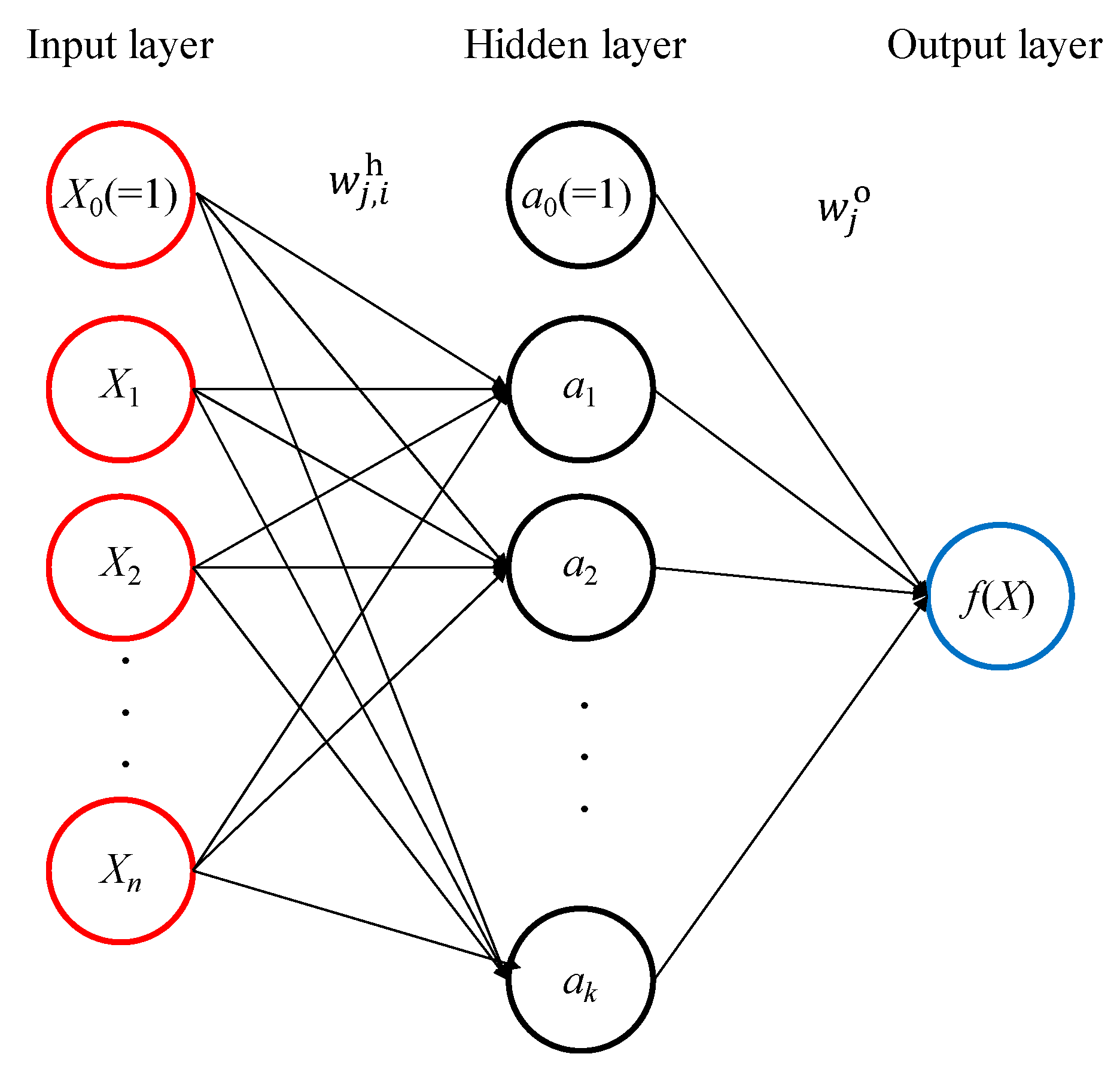
2.2. Overview of Multilayer Perceptron in an Artificial Neural Network

Figure 1 shows a schematic diagram of the MLP network. The MLP is a hierarchical network comprising an input layer, a hidden layer, and an output layer; the unit of the hidden layer is completely connected to the input and output layers [34,35].

In Figure 1, only one hidden layer is schematically shown; however, in general, multiple hidden layers are used to enhance the expressiveness of the model. The unit in the hidden layer (hereinafter, referred to as the activation unit a_j (j = 1~k)) is calculated using Equation (1), where n input values are X_i and the output values are f(X).

$$a_j=\varphi \left({\displaystyle \sum }_{i=0}^n{w}_{j,i}^{\mathrm{h}}{X}_i\right)$$

(1)

Here, $w_{j,i}^{\mathrm{h}}$ is the connection weight, X₀ is a constant called bias, and $\varphi$ of Equation (1) is a function called the activation function. For the activation function, a function with differentiable nonlinearity was selected to enhance the expressiveness of the model. In this study, the rectified linear unit (ReLU) function $\varphi$(z) = max(0, z) was used and a_j was assigned to the hidden layer. The total number k of a_j (the number of nodes in the hidden layer) and the number of hidden layers are parameters that were adjusted according to the learning accuracy. The output value f(X) can be obtained via Equation (2).

$$f\left(X\right)=\varphi \left({{\displaystyle \sum }}_{j=0}^k{w}_j^{\mathrm{o}}{a}_j\right),$$

(2)

where $w_j^{\mathrm{o}}$ denotes the connection weight. In Equations (1) and (2), the connection weights $w_{j,i}^{\mathrm{h}},w_j^{\mathrm{o}}$ are unknown constants and can be obtained from the combination of known input and output values. By assuming that the known teaching data (true value) are Y (to distinguish it from f(X), predicted from the input value X_i from Equation (2)), the connection weights can be updated in Equation (3), using the loss function E.

$$E=\frac{1}{2}{\displaystyle \sum }_l{(Y_l-f_l\left(X\right))}^2+\frac{\alpha }{2}{\displaystyle \sum }_l{\left|w_l^{\mathrm{o}}\right|}^2$$

(3)

Here, the first term in Equation (3) is the sum of the squared residuals of the teaching data Y and the output value f(X), and the second term is a regularization term using the L² norm to suppress overfitting. α is a parameter that is adjusted according to learning accuracy. Overfitting is a problem in which training data are overfitted and unknown data cannot be effectively generalized. Several effective optimization algorithms have been developed to avoid falling into a locally optimal solution for updating the connection weights. In this study, adaptive moment estimation (Adam) [36] was used. The connection weight w is updated using Equations (4)–(9).

$$W^{\left(t\right)}=w^{\left(t-1\right)}-\eta \frac{\widehat{m^{\left(t\right)}}}{\sqrt{\widehat{v^{\left(t\right)}}}+ϵ}$$

(4)

$$\widehat{m^{\left(t\right)}}=\frac{m^{\left(t\right)}}{1-{\beta }_1^t}$$

(5)

$$\widehat{v^{\left(t\right)}}=\frac{v^{\left(t\right)}}{1-{\beta }_2^t}$$

(6)

$$m^{\left(t\right)}={\beta }_1{m}^{\left(t-1\right)}+\left(1-{\beta }_1\right)\frac{\partial E}{\partial w}$$

(7)

$$v^{\left(t\right)}={\beta }_2{v}^{\left(t-1\right)}+\left(1-{\beta }_2\right){\left(\frac{\partial E}{\partial w}\right)}^2$$

(8)

$$m^{\left(0\right)}=v^{\left(0\right)}=0$$

(9)

The recommended values were used for the adjustment parameters η, β₁, β₂, and $ϵ$ [36]. The error backpropagation method to update the connection weight was used, which calculates the gradient of the loss function by moving backward from the output layer. This method is known to be less computationally expensive than updating weights in the forward direction [37].

2.3. Goodness Valuation of Constructed Learning Model

The goodness of valuation of the constructed machine learning model is based on the coefficient of determination R² in Equation (10), where n is the amount of teaching data, Y_i is the true objective value, f(X) is the predicted objective value, and the average value of the true objective values is σ_Y.

$$R^2=1-\frac{{{\displaystyle \sum }}_i{(Y_i-f_i\left(X\right))}^2}{{{\displaystyle \sum }}_i{\left(Y_i-{\mu }_{\mathrm{Y}}\right)}^2}$$

(10)

The coefficient of determination indicates the goodness of fit of the regression model and is an evaluation index for assessing how well the predicted and true values match. R² = 1 when the true and predicted values are the same. There is no clear standard for the coefficient of determination, but it can be considered compatible if it is approximately 0.5 or more.

2.4. Dataset

For machine learning, the fracture toughness test data of 531 ferritic steels in the DBTT region obtained by the authors or previous studies were used.

Table 1. Chemical compositions of the test specimens (wt %) of the considered materials.

Heat No.	Material	C	Si	Mn	P	S	Ni	Cr	Mo	V	Cu	Nb	Ti	Al
1	MiuraSFVQ1A [38]	0.18	0.18	1.46	0.002	<0.001	0.90	0.12	0.52	<0.01	-	-	-	-
		0.17	0.17	1.39	0.002	<0.001	0.87	0.11	0.50	<0.01	-	-	-	-
2	Gopalan20MnMoNi55 [39]	0.20	0.24	1.38	0.011	0.005	0.52	0.06	0.30	-	-	0.032	-	0.068
3	ShorehamA533B [40]	0.21	0.24	1.23	0.004	0.008	0.63	0.09	0.53	-	0.08	-	-	0.04
4	MiuraSQV2Ah1 [38]	0.22	0.25	1.44	0.021	0.028	0.54	0.08	0.48	-	0.10	-	-	-
5	MiuraSQV2Ah2 [38]	0.22	0.25	1.46	0.002	0.002	0.69	0.11	0.57	-	-	-	-	-
6	GarciaS275JR [41]	0.18	0.26	1.18	0.012	0.009	<0.085	<0.018	<0.12	<0.02	0.06	-	0.022	0.034
7	GarciaS355J2 [41]	0.2	0.31	1.39	<0.012	0.008	0.09	0.05	<0.12	0.02	0.06	-	0.022	0.014
8	CiceroS460M [42]	0.12	0.45	1.49	0.012	0.001	0.016	0.062	-	0.066	0.011	0.036	0.003	0.048
9	CiceroS690Q [42]	0.15	0.40	1.42	0.006	0.001	0.160	0.020	-	0.058	0.010	0.029	0.003	0.056
10	MeshiiFY2017SCM440 [25]	0.39	0.17	0.62	0.011	0.002	0.07	1.02	0.17	-	0.10	-	-	-
11	MeshiiFY2012S55C [6]	0.55	0.17	0.61	0.015	0.004	0.07	0.08	-	-	0.13	-	-	-
12	MeshiiFY2016S55C [26]	0.54	0.17	0.61	0.014	0.003	0.06	0.12	-	-	-	-	-	-

presents the chemical compositions of the test specimens of the materials considered in the teaching data.

Table 2. K_Jc data used to construct the proposed tensile property-based MC: RPV steel ASTM A508 equivalent.

Heat No.	Material	Specimen	Temps.	Num. of Temps.	σYS	σYSRT	σBRT	Num. of Specimens	T0
		Type	(°C)		(MPa)	(MPa)	(MPa)		(°C)
1	MiuraSFVQ1A [38]	1TC(T)	−120~−60	4	530~640	454	594	32	−98
		2TC(T)	−120~−60	4	530~640	454	594	16	−98
		4TC(T)	−100~−80	2	560~607	454	594	12	−98
		0.4TC(T)	−140~−80	4	560~695	454	594	34	−98
		0.4TSE(B)	−140~−80	4	560~695	454	594	29	−98
2	Gopalan20MnMoNi55 [39]	1TC(T)	−140~−80	3	560~667	479	616	18	−133
		0.5TC(T)	−140~−80	3	560~667	479	616	12	−133

,

Table 3. K_Jc data used to construct the proposed tensile property-based K_Jc MC: RPV steel ASTM A533B and equivalent.

Heat No.	Material	Specimen	Temps.	Num. of Temps.	σYS	σYSRT	σBRT	Num. of Specimens	T0
		Type	(°C)		(MPa)	(MPa)	(MPa)		(°C)
3	ShorehamA533B [40]	1TC(T) *	−100~−64	3	551~586	488	644	18	−91
4	MiuraSQV2Ah1 [38]	1TC(T)	−100~−60	3	544~600	473	625	14	-93
		2TC(T)	−100~−60	3	544~600	473	625	14	−93
		4TC(T)	−80~−60	2	544~566	473	625	12	−93
		0.4TC(T)	−120~−60	4	544~658	473	625	32	−93
		0.4TSE(B)	−120~−60	4	544~658	473	625	29	−93
5	MiuraSQV2Ah2 [38]	1TC(T)	−140~−80	4	542~709	461	602	23	−121
		2TC(T)	−100~−80	2	542~607	461	602	12	−121
		4TC(T)	−100~−80	2	542~607	461	602	12	−121
		0.4TC(T)	−140~−80	4	542~709	461	602	33	−121
		0.4TSE(B)	−140~−80	4	542~709	461	602	32	−121

*: Side-grooved specimens.

and

Table 4. K_Jc data used to construct the proposed tensile property-based MC: non-RPV steels.

Heat No.	Material	Specimen	Temps.	Num. of Temps.	σYS	σYSRT	σBRT	Num. of Specimens	T0
		Type	(°C)		(MPa)	(MPa)	(MPa)		(°C)
6	GarciaS275JR [41]	1TC(T)	−50~−10	3	338~349	328	519	14	−26
7	GarciaS355J2 [41]	1TC(T)	−150~−100	3	426~528	375	558	13	−134
8	CiceroS460M [42]	0.6TSE(B)	−140~−100	3	597~686	473	595	14	−92
9	CiceroS690Q [42]	0.6TSE(B)	−140~−100	3	899~988	775	832	13	−111
10	MeshiiFY2017SCM440 [25,30]	0.9TSE(B)	−55~100	4	410~524	459	796	18	17
		0.5TSE(B)	−55~100	4	410~524	459	796	22	17
11	MeshiiFY2012S55C [6]	0.5TSE(B)	−25~20	3	394~444	394	707	17	27
12	MeshiiFY2016S55C [26,30]	0.9TSE(B)	−45~35	3	375~475	382	685	17	15
		0.5TSE(B)	−85~20	3	382~562	382	685	19	15

summarize the material heats (heat No. 1–12) used in this study, nT indicates the specimen thickness, and n is expressed in multiples of 25 mm. They are fundamentally extracted from previous work [30,33], but differ slightly in terms of the following: (1) K_Jc > K_Jc(ulimit) invalid data were excluded, (2) K_Jc data were limited to cases obtained with standard specimens of thickness-to-width ratio B/W = 0.5, (3) When there were no σ_YS data for the fracture toughness test temperature, it was obtained by using the following modified Z–A σ_YS temperature-dependent MC [9]

$${\sigma }_{0\mathrm{ZA}}\left(T\right)={\sigma }_{0\mathrm{RT}}+C_{1}exp\left[\left(T+273.15\right)\left(-C_3+C_4\log \left(\dot{\epsilon }\right)\right)\right]-49.6 \left(\mathrm{MPa}\right),$$

(11)

where T is the temperature (°C), C₁ = 1033 (MPa), C₃ = 0.00698 (1/K), C₄ = 0.000415 (1/K), and $\dot{\epsilon }$ = 0.0004 (1/s). The three Miura heats (heat No. 1, 4, 5) were another exception for which linear interpolation of raw data was used because the fracture toughness and tensile test temperatures were different.

The objective variable was K_Jc. Assuming a direct relationship between the SED temperature dependence and that of K_Jc, σ_B temperature dependence was the first candidate explanatory parameter. However, considering that (i) σ_B/σ_YS temperature dependence is small, (ii) ferritic steel has a σ_YS temperature-dependent MC such as Z−A MC, and (iii) σ_B/σ_YS at RT is usually easily available, σ_B and σ_YS at RT, and σ_YS at K_Jc test temperatures and specimen width W were selected as the explanatory variables. To optimize the connection weight, 371 points, i.e., 70% of the 531 points in the known dataset, were used as the training data. The data were divided by “train_test_split” of Python’s scikit-learn library. If the digits of the input value and output value to be learned are significantly different, the influence of variables with small digits may not be fully considered in learning. Therefore, in this study, the input values W, σ_YS, σ_YSRT, σ_BRT, and output value K_Jc were standardized, as shown in Equation (12).

$$\left(\begin{array}{c}W \left(\mathrm{mm}\right)\\ {\sigma }_{\mathrm{YS}} \left(\mathrm{MPa}\right)\\ {\sigma }_{\mathrm{YSRT}} \left(\mathrm{MPa}\right)\\ {\sigma }_{\mathrm{BRT}} \left(\mathrm{MPa}\right)\\ K_{J\mathrm{c}} \left({\mathrm{MPa}·\mathrm{m}}^{1/2}\right)\end{array}\right)\stackrel{\mathrm{Normalized}}{\to }\left(\begin{array}{c}W/50\\ {\sigma }_{\mathrm{YS}}/550\\ {\sigma }_{\mathrm{YSRT}}/550\\ {\sigma }_{\mathrm{BRT}}/550\\ K_{J\mathrm{c}}/100\end{array}\right)$$

(12)

Here, with reference to ASTM E1921, W was normalized using the width 50 mm of a 1T specimen, and the yield stress and tensile strength were normalized using the average value of 550 MPa of the yield stress of 275 to 825 MPa in the allowable temperature range targeted by the standard. K_Jc was normalized to a fracture toughness of value 100 MPa·m^1/2 at the reference temperature.

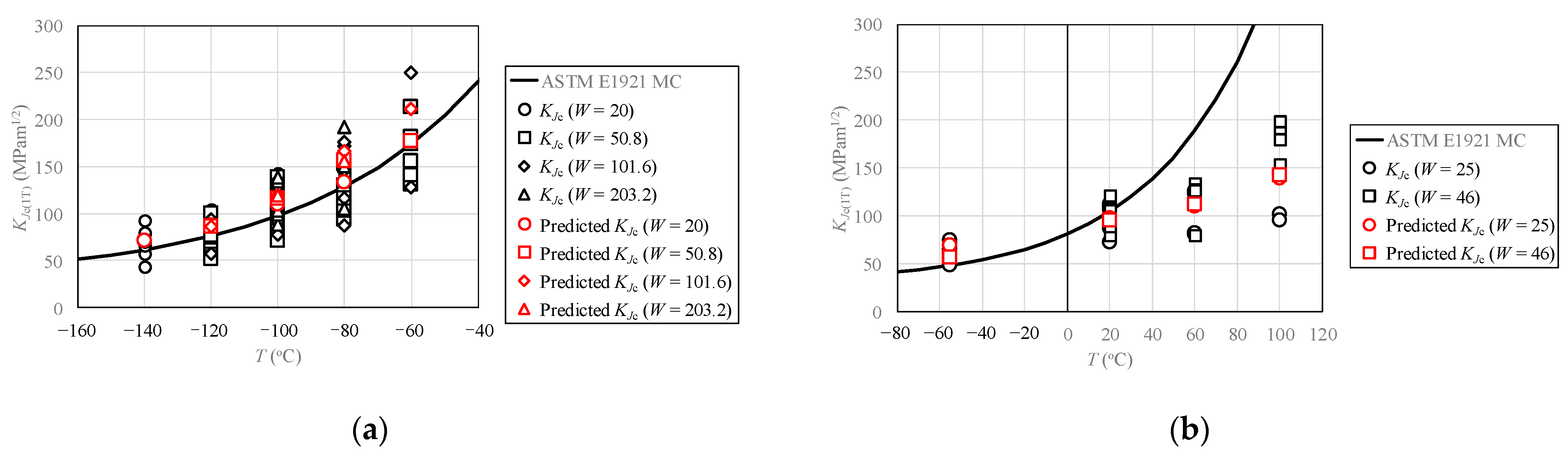
2.5. Fracture Toughness Prediction by the Constructed Learning Model

Table 5. Hyperparameters used for the learning model.

Parameters	Value
Number of hidden layers	4
Number of hidden layer nodes	100, 50, 25, 10
Activation function	ReLU
Solver	Adam
α	0.01
η	0.001
β1	0.9
β2	0.999
$ϵ$	1.0 × 10−8

presents a list of hyperparameters used for the machine learning model in this study. Using the data in Table 2, Table 3 and Table 4 and the parameters in Table 5, which is currently an invariant model, the coefficient of determination R² of the developed K_Jc predictor was 0.61 for the training data and 0.53 for the test data.

Table 6. Explanatory variables for case studies applied to the developed tool.

Heat No.	Material	W (mm)	T (°C)	σYSRT (MPa)	σYS (MPa)	σBRT (MPa)
1	Miura SFVQ1A	20	−140, −120, −100, −80	454	695, 640, 607, 560	594
		50.8	−120, −100, −80, −60	454	640, 607, 560, 530	594
		101.6	−120, −100, −80, −60	454	640, 607, 560, 530	594
		203.2	−80, −100	454	607, 560	594
10	MeshiiFY2017SCM440	25	−55, 20, 60 100	459	524, 459, 435, 410	796
		46	−55, 20, 60, 100	459	524, 459, 435, 410	796

presents the explanation variables for predicting fracture toughness K_Jc.

The input data (W, σ_YS, σ_YSRT, σ_BRT) for the developed K_Jc predictor and output window after its execution (the coefficient of determination R² and the predicted K_Jc) are shown in Figure 2. In Figure 3, the comparison of K_Jc of ASTM E1921 MC and predicted K_Jc by the predictor is shown. In Figure 3, the horizontal axis is T, the vertical axis K_Jc(1T) is the test data, and the predicted K_Jc is converted to 1T thickness. The K_Jc of the ASTM E1921 MC is plotted as a black solid line, the K_Jc of the test data are plotted as open black symbols, and the predicted conditions listed in Table 6 are plotted as open red symbols. In Figure 3a, for RPV steel, both the K_Jc by the ASTM E1921 MC and the predicted K_Jc by this model are in agreement with the test results. However, in Figure 3b for SCM440, although the K_Jc by the ASTM E1921 MC significantly differs from the test results at high temperatures, the predicted K_Jc values by this model are in agreement with the test results.

3. Discussion

By applying the ANN, a K_Jc predictor for ferritic steels that only requires tensile properties (i.e., σ_YS at the desired temperature for predicting K_Jc, and the RT values σ_YSRT and σ_BRT) were derived. This method eliminates the need for time- and material-consuming fracture toughness tests. The tool for predicting K_Jc by considering the specimen size and material properties is based on 531 fracture toughness test data values obtained from five RPV steel heats and seven non-RPV steel heats. The specimen sizes ranged from 0.4T to 4T to learn the size effect, the yield stress ranged from 328 to 775, and the tensile strength ranged from 519 to 832 to learn the material properties. The data range used in the training was equal to the application limit of the predictor. The developed K_Jc predictor successfully predicted training data with R² = 0.61 and test data with R² = 0.53.

To predict K_Jc at a specific temperature of interest, the user needs σ_YS at this temperature as well as σ_YSRT and σ_BRT at RT. If the material of interest is known to be well fitted by the Z–A σ_YS MC, the quantities for which test data are necessary for K_Jc prediction are only σ_YSRT and σ_BRT.

A considerable advantage of the proposed K_Jc predictor is that fracture toughness tests are not necessary to predict K_Jc. The key novel idea here is to use tensile properties (such as σ_YS and σ_B) and specimen size W.

Although the developed K_Jc predictor predicts one K_Jc for a combination of explanatory variables, the predicted K_Jc fracture probability is predicted by assuming the probability distribution of the data to be learned (e.g., Weibull distribution). It is also possible to evaluate it together, which is a future issue.

According to Table 2, Table 3 and Table 4, the (σ_B/σ_YS)_RT of non-RPV and RPV are different. Accepting Kirk’s opinion that K_Jc and SED correspond, ASTM E1921 MC may deviate from non-RPV. However, this K_Jc predictor has an advantage in that it considers this. On this point, the developed K_Jc predictor, compared with the existing ASTM E1921 K_Jc MC, is expected to be especially effective in cases where σ_B/σ_YS of the material is larger than that of RPV steel.

The predictors that were generated and analyzed during the current study are available from the corresponding author upon reasonable request.

4. Conclusions

In this study, a tool was developed that can predict K_Jc for an arbitrary specimen size W and material properties (σ_YSRT, σ_YS, σ_BRT) via an ANN applied to 531 fracture toughness test data values. Currently, the conditions applicable to the tool are material properties ranging from σ_YSRT = 328 to 775 MPa, σ_BRT = 519 to 832 MPa, specimen size ranging from 0.4T to 4T and its types are CT and SEB. By using the tool developed through the application of data-driven ideas, it is possible to predict the fracture toughness at this temperature from the tensile test results and the specimen size at the target temperature of the fracture toughness without performing a fracture toughness test. In the future, it is planned to predict the predicted probability of fracture toughness.

References

1. James, P.M.; Ford, M.; Jivkov, A.P. A novel particle failure criterion for cleavage fracture modelling allowing measured brittle particle distributions. Eng. Fract. Mech. 2014, 121–122, 98–115. [Google Scholar] [CrossRef]
2. ASTM E1921-10. Standard Test Method for Determination of Reference Temperature, T0, for Ferritic Steels in the Transition Range; American Society for Testing and Materials: Philadelphia, PA, USA, 2010. [Google Scholar]
3. Odette, G.R.; He, M.Y. A cleavage toughness master curve model. J. Nucl. Mater. 2000, 283, 120–127. [Google Scholar] [CrossRef]
4. Ritchie, R.O.; Knott, J.F.; Rice, J.R. On the relationship between critical tensile stress and fracture toughness in mild steel. J. Mech. Phys. Solids 1973, 21, 395–410. [Google Scholar] [CrossRef]
5. Curry, D.A.; Knott, J.F. The relationship between fracture toughness and microstructure in the cleavage fracture of mild steel. Met. Sci. 1976, 10, 1–6. [Google Scholar] [CrossRef]
6. Ishihara, K.; Hamada, T.; Meshii, T. T-scaling method for stress distribution scaling under small-scale yielding and its application to the prediction of fracture toughness temperature dependence. Theor. Appl. Fract. Mech. 2017, 90, 182–192. [Google Scholar] [CrossRef]
7. Wallin, K. Irradiation damage effects on the fracture toughness transition curve shape for reactor pressure vessel steels. Int. J. Press. Vessels Pip. 1993, 55, 61–79. [Google Scholar] [CrossRef]
8. ASTM E1921-19b. Standard Test Method for Determination of Reference Temperature, T0, for Ferritic Steels in the Transition Range; American Society for Testing and Materials: Philadelphia, PA, USA, 2019. [Google Scholar]
9. Kirk, M.T.; Natishan, M.; Wagenhofer, M. Microstructural limits of applicability of the master curve. In Fatigue and Fracture Mechanics; Chona, R., Ed.; American Society for Testing and Materials: Philadelphia, PA, USA, 2001; Volume 32, pp. 3–16. [Google Scholar]
10. Kirk, M.T. The Technical Basis for Application of the Master Curve to the Assessment of Nuclear Reactor Pressure Vessel Integrity; ADAMS ML093540004; United States Nuclear Regulatory Commission: Washington, DC, USA, 2002.
11. Wallin, K. The size effect in KIC results. Eng. Fract. Mech. 1985, 22, 149–163. [Google Scholar] [CrossRef]
12. Dodds, R.H.; Anderson, T.L.; Kirk, M.T. A framework to correlate a/W ratio effects on elastic-plastic fracture toughness (Jc). Int. J. Fract. 1991, 48, 1–22. [Google Scholar] [CrossRef]
13. Kirk, M.T.; Dodds, R.H.; Anderson, T.L. An approximate technique for predicting size effects on cleavage fracture toughness (Jc) using the elastic T stress. In Fracture Mechanics; Landes, J.D., McCabe, D.E., Boulet, J.A.M., Eds.; American Society for Testing and Materials: Philadelphia, PA, USA, 1994; Volume 24, pp. 62–86. [Google Scholar]
14. Rathbun, H.J.; Odette, G.R.; He, M.Y.; Yamamoto, T. Influence of statistical and constraint loss size effects on cleavage fracture toughness in the transition—A model based analysis. Eng. Fract. Mech. 2006, 73, 2723–2747. [Google Scholar] [CrossRef]
15. Meshii, T.; Lu, K.; Takamura, R. A failure criterion to explain the test specimen thickness effect on fracture toughness in the transition temperature region. Eng. Fract. Mech. 2013, 104, 184–197. [Google Scholar] [CrossRef]
16. Meshii, T.; Yamaguchi, T. Applicability of the modified Ritchie-Knott-Rice failure criterion to transfer fracture toughness Jc of reactor pressure vessel steel using specimens of different thicknesses–possibility of deterministic approach to transfer the minimum Jc for specified specimen thicknesses. Theor. Appl. Fract. Mech. 2016, 85, 328–344. [Google Scholar] [CrossRef]
17. Anderson, T.L.; Stienstra, D.; Dodds, R.H. A theoretical framework for addressing fracture in the ductile-brittle transition region. In Fracture Mechanics; Landes, J.D., McCabe, D.E., Boulet, J.A.M., Eds.; American Society for Testing and Materials: Philadelphia, PA, USA, 1994; Volume 24, pp. 186–214. [Google Scholar]
18. Yang, S.; Chao, Y.J.; Sutton, M.A. Higher order asymptotic crack tip fields in a power-law hardening material. Eng. Fract. Mech. 1993, 45, 1–20. [Google Scholar] [CrossRef]
19. Meshii, T.; Tanaka, T. Experimental T33-stress formulation of test specimen thickness effect on fracture toughness in the transition temperature region. Eng. Fract. Mech. 2010, 77, 867–877. [Google Scholar] [CrossRef]
20. Matvienko, Y.G. The effect of out-of-plane constraint in terms of the T-stress in connection with specimen thickness. Theor. Appl. Fract. Mech. 2015, 80, 49–56. [Google Scholar] [CrossRef]
21. Matvienko, Y.G. The effect of crack-tip constraint in some problems of fracture mechanics. Eng. Fail. Anal. 2020, 110, 104413. [Google Scholar] [CrossRef]
22. Beremin, F.M.; Pineau, A.; Mudry, F.; Devaux, J.C.; D’Escatha, Y.; Ledermann, P. A local criterion for cleavage fracture of a nuclear pressure vessel steel. Metall. Mater. Trans. A 1983, 14, 2277–2287. [Google Scholar] [CrossRef]
23. Khalili, A.; Kromp, K. Statistical properties of Weibull estimators. J. Mater. Sci. 1991, 26, 6741–6752. [Google Scholar] [CrossRef]
24. Zerilli, F.J.; Armstrong, R.W. Dislocation-mechanics-based constitutive relations for material dynamics calculations. J. Appl. Phys. 1987, 61, 1816–1825. [Google Scholar] [CrossRef] [Green Version]
25. Meshii, T. Failure of the ASTM E 1921 master curve to characterize the fracture toughness temperature dependence of ferritic steel and successful application of the stress distribution T-scaling method. Theor. Appl. Fract. Mech. 2019, 100, 354–361. [Google Scholar] [CrossRef]
26. Meshii, T. Spreadsheet-based method for predicting temperature dependence of fracture toughness in ductile-to-brittle temperature region. Adv. Mech. Eng. 2019, 11, 1–17. [Google Scholar] [CrossRef]
27. Zerbst, U.; Heerens, J.; Pfuff, M.; Wittkowsky, B.U.; Schwalbe, K.H. Engineering estimation of the lower bound toughness in the transition regime of ferritic steels. Fatigue Fract. Eng. Mater. Struct. 1998, 21, 1273–1278. [Google Scholar] [CrossRef]
28. Heerens, J.; Pfuff, M.; Hellmann, D.; Zerbst, U. The lower bound toughness procedure applied to the Euro fracture toughness dataset. Eng. Fract. Mech. 2002, 69, 483–495. [Google Scholar] [CrossRef] [Green Version]
29. Lu, K.; Meshii, T. Application of T33-stress to predict the lower bound fracture toughness for increasing the test specimen thickness in the transition temperature region. Adv. Mater. Sci. Eng. 2014, 1–8. [Google Scholar] [CrossRef] [Green Version]
30. Meshii, T. Characterization of fracture toughness based on yield stress and successful application to construct a lower-bound fracture toughness master curve. Eng. Fail. Anal. 2020, 116, 104713. [Google Scholar] [CrossRef]
31. Akbarzadeh, P.; Hadidi-Moud, S.; Goudarzi, A.M. Global equations for Weibull parameters in a ductile-to-brittle transition regime. Nucl. Eng. Des. 2009, 239, 1186–1192. [Google Scholar] [CrossRef]
32. Wenman, M.R. Fitting small data sets in the lower ductile-to-brittle transition region and lower shelf of ferritic steels. Eng. Fract. Mech. 2013, 98, 350–364. [Google Scholar] [CrossRef]
33. Meshii, T.; Yakushi, G.; Takagishi, Y.; Fujimoto, Y.; Ishihara, K. Quantitative comparison of the predictions of fracture toughness temperature dependence using ASTM E1921 master curve and stress distribution T-scaling methods. Eng. Fail. Anal. 2020, 111, 104458. [Google Scholar] [CrossRef]
34. Scikit-Learn. Available online: https://scikit-learn.org/stable/index.html (accessed on 13 October 2021).
35. Raschka, S.; Mrjalili, V. Python Machine Learning, 2nd ed.; Packt Publishing: Birmingham, UK, 2017. [Google Scholar]
36. Kingma, D.P.; Ba, J.L. ADAM: A METHOD FOR STOCHASTIC OPTIMIZATION. In Proceedings of the 3rd International Conference for Learning Representations, San Diego, CA, USA, 7–9 May 2015. [Google Scholar]
37. Rumelhart, D.E.; Hinton, G.E.; Williams, R.J. Learning representations by back-propagating errors. Nature 1986, 323, 533–536. [Google Scholar] [CrossRef]
38. Miura, N. Study on Fracture Toughness Evaluation Method for Reactor Pressure Vessel Steels by Master Curve Method Using Statistical Method. Ph.D. Thesis, The University of Tokyo, Tokyo, Japan, 2014. (In Japanese). [Google Scholar]
39. Gopalan, A.; Samal, M.K.; Chakravartty, J.K. Fracture toughness evaluation of 20MnMoNi55 pressure vessel steel in the ductile to brittle transition regime: Experiment & numerical simulations. J. Nucl. Mater. 2015, 465, 424–432. [Google Scholar] [CrossRef]
40. Rathbun, H.J.; Odette, G.R.; Yamamoto, T.; Lucas, G.E. Influence of statistical and constraint loss size effects on cleavage fracture toughness in the transition—A single variable experiment and database. Eng. Fract. Mech. 2006, 73, 134–158. [Google Scholar] [CrossRef]
41. García, T.; Cicero, S. Application of the master curve to ferritic steels in notched conditions. Eng. Fail. Anal. 2015, 58, 149–164. [Google Scholar] [CrossRef]
42. Cicero, S.; García, T.; Madrazo, V. Application and validation of the notch master curve in medium and high strength structural steels. J. Mech. Sci. Technol. 2015, 29, 4129–4142. [Google Scholar] [CrossRef] [Green Version]
Figure 1. Schematic diagram of multilayer perceptron in an ANN [35].
Metals 11 01740 g001
Figure 2. Input data (left figure) and window after execution (right figure). (a) Input data; (b) Output window.
Metals 11 01740 g002
Figure 3. Comparison of KJc of ASTM E1921 MC (solid line) and predicted KJc by the predictor (open red symbols): Dataset used for training model and result of predicted KJc. (a) RPV steel (Miura SFVQ1A); (b) Meshii FY2017SCM440. KJc pre-dicted by the developed predictor accurately predicted KJc regardless of materials.
Metals 11 01740 g003