Effects of Impeller Rotational Speed and Immersion Depth on Flow Pattern, Mixing and Interface Characteristics for Kanbara Reactors Using VOF-SMM Simulations

Abstract

The Kanbara Reactor (KR) is a primary desulfurization technology in the hot metal pretreatment refining process that is widely employed in the modern steelmaking industry. The operating parameters of KR impeller immersion depth (IID) and rotation speed (IRS) have a crucial impact on the process performance and the desulfurization effect. Still, their influences have not been fully understood. This study systematically investigated the effects of IID and IRS on the flow pattern, mixing behavior, vortex core depth, and free surface characteristics for KR processes based on a 3D Volume of Fluid (VOF) model coupled with the sliding mesh method (SMM). The model was validated via scale-down water model experiments and then applied to the KR process, and simulations found that IID and IRS have different impacts on the flow pattern. Specifically, the discharge flow location moves downward with IID increasing, but the discharge strength and mean velocity hardly changes. Comparatively, the rise of IRS significantly increases the mean velocity, but few changes occur to the discharge flow position. Increasing IRS improves bath hydrodynamics, strengthens recirculation, and efficiently shortens mixing time, but IID has a neglectable effect on these features. The minimum mixing time is 55 s at a maximum IRS of 260 rpm. Moreover, the vortex core depth and free surface velocity visibly increase with the increase of IRS. Comparatively, IID has a limited effect on the flow and mixing behavior but directly impacts the distribution of recirculation regions at the axial direction and the velocity gradient on the free surface at the radial direction. Furthermore, the correlation equations of these critical parameters as a function of the operating parameters were obtained. The results from this study may provide references for operating optimizations and industrial practices of KRs.

1. Introduction

With the increasing demand for high-quality steel, cleanliness is of paramount importance in each stage of steel refining and production. Except for special applications, the sulfur existing in products is usually a detrimental impurity that adversely affects the temperature toughness, weldability, and hydrogen-induced cracking resistance during the service life of products [1,2]. Thus, it is essential to reduce the sulfur content to as low as possible to satisfy the specification of the product. Desulfurization is usually carried out before the hot metal is mixed into the converter because of favorable thermodynamic conditions, and this stage is thus called the pretreatment procedure for desulfurization. Approaches used here can be classified into two categories: mechanically stirred and powder injection (PI). Among them, the Kanbara Reactor (KR) [3], as a typical mechanically stirred method (MSM) [4,5,6], has significant advantages with high efficiency, short treatment time, and lower cost, providing the intensely hydrodynamic conditions through the revolving motion of a submerged impeller. Practically, the rotational speed and immersion depth of the impeller, as two vital operating parameters, remarkably impact the entrainment of the reagent powder, mixing characteristics, and refining efficiency, as well as the service life of an impeller and the ladle because of higher refractory wear induced by the washing of revolving, high-temperature metal.

Some studies have been conducted on different aspects of MSM or KRs, including fluid flows, bath mixing behaviors, reagent dispersion, and impeller design based on scale-down water models, numerical simulations, and laboratory-scale high-temperature experiments. For example, Visuri et al. [1] have given a recent review in modeling hot metal desulfurization and summarized the previous contributions and work on fluid flow phenomena, mixing patterns, and particle/bubble dispersions in KR processes. Yamamoto et al. [7,8] investigated the flow characteristic of aluminum melt by mechanically stirring and found that the impeller depths, rotation speeds, and impeller twisting angles impact the mixing time. Kato et al. [9] evaluated the flow pattern and mass transfer in an aluminum melting furnace using a numerical simulation. They found that the region with high kinetic energy was enlarged, and the turbulent kinetic energy at the free surface increased significantly with impeller rotation speed. This result illustrated that increasing impeller rotation speed is an effective method to enhance the mass transfer behavior of reactors. Their more recent research [10] found that increasing rotation speed would increase vortex depth and the intensity of turbulent fluctuations on the free surface. He et al. [11] investigated the coalescence and sedimentation behavior of falling droplets in a vessel of MSM. They found that increasing rotation speed is conducive to the dispersion of droplets in the mechanical stirring vessel. Later, they [12] also investigated the dispersed behavior of desulfurization particles at different rotation speeds and found that rotation speed affects the liquid dispersion in the mechanical stirring vessel and has a noticeable effect on the distribution of particles in the hot metal. Li et al. [13,14] used a Volume of Fluid with a dispersed particle model (VOF-DPM) to analyze the drawdown mechanism and the dispersion characteristic of light particles at different rotation speeds. They found that a higher impeller rotation speed can provide more power consumption and increase particle velocity, which means the mixing efficiency would be better. Nakai et al. [15,16] described the variation of the gas–liquid interface at different stages of the mixing process in a 1/8 scale water model. They found that the vortex height and operation parameters, such as impeller immersion depths, rotation speeds, and the geometric size of KR, have a relationship. Ji et al. [17] investigated the mixing behavior of KR vessels using computational fluid dynamics (CFD) simulations. By comparing fixed- and variable-velocity stirring, they found the latter stirring mode to be more favorable in the mixing of a bath. Sahu et al. [18] used CFD simulation, which optimized the operating parameters in the synthesis of hybrid aluminum matrix composites by stir casting. They found that blade angle, impeller size, and stirring speed are the typical factors that affect the flow pattern. Liu et al. [19] investigated impeller immersion depths, rotation speeds, and eccentric mechanical stirring modes. They found that increasing rotation speed can effectively strengthen the shear effect around the impeller, which intensifies bubble disintegration and dispersion. With an increasing impeller immersion depth, the distance between the vortex and impeller rises gradually. All the related research above shows that the impeller immersion depth and rotation speed significantly influence the fluid flow and mixing efficiency. However, to date, only a few reports focus on this topic, and it is not fully understood or well documented due to the limits of the measurement method and high costs of in-situ experimentation at a high ambient temperature and within a hazardous environment.

This study aims to provide a detailed analysis of the effect of impeller operating variables on fluid flow pattern, mixing characteristics, vortex core depth, and free surface velocity of KRs based on the developed Volume of Fluid model with the sliding mesh method (VOF-SMM). This study extends our previous work [20] in which the effect of the impeller dimension was discussed. Here, our focus is the rotational speed and immersion depth of impellers.

2. Mathematical Model

Our model has been reported in recent studies on the effect of impeller dimension for the KR process [20] and on a new dephosphorization technology for the converter steelmaking process [21]. In those studies, the grid sensitivity, calibration of the turbulence model, and model validation have been carefully examined, but considering some improvements and the completion of the present work, the outline is given as follows.

2.1. Governing Equations of VOF Model

To track the free surface of gas–liquid two-phase flow in a KR, some assumptions were specified, and details were given in our previous work [20]. As a result, the hydrodynamics of this multiphase system is governed by a set of single Navier–Stokes equations and a continuity equation.

$$\frac{\partial \rho }{\partial t}+\frac{\partial \left(\rho u_i\right)}{\partial x_i}=0$$

(1)

$$\frac{\partial \rho u_i}{\partial t}+\frac{\partial \left(\rho u_i{u}_j\right)}{\partial x_j}=-\frac{\partial p}{\partial x_i}+\frac{\partial {\tau }_{ij}^{}}{\partial x_j}+\rho g_i+f_{\mathsf{\sigma }}$$

(2)

Here, u_i and u_j are the velocity components in the direction of i and j, respectively (m·s⁻¹); t is the time (s); p is the pressure (Pa); g is the gravity acceleration (m·s⁻²); and τ_ij is the Reynold stress tensor (N·m⁻²), which is calculated as follows:

$${\mathsf{\tau }}_{ij}={\mu }_{\mathrm{eff}}\left(\frac{\partial u_j}{\partial x_i}+\frac{\partial u_i}{\partial x_j}\right)-\frac{2}{3}{\mu }_{\mathrm{eff}}\frac{\partial u_k}{\partial x_k}{\delta }_{ij}$$

(3)

where δ_ij is the Kronecker delta (δ_ij = 1 if I = j and δ_ij = 0 if i ≠ j); μ_eff is the effective viscosity (Pa·s) calculated by:

$${\mu }_{\mathrm{eff}}=\mu +{\mu }_{\mathrm{t}}$$

(4)

where μ is the molecular viscosity (Pa·s) and the turbulent viscosity μ_t (Pa·s) is calculated by the turbulence model.

In the present study, a modified approach was used based on the multi-fluid formulation proposed by Ubbink and Isssa [22]. The evolution of the interface/free surface [23] is described by an additional transport equation for the indicator function representing the volume fraction of one phase that needs to be solved together with the continuity and momentum equations:

$$\frac{\partial {\alpha }_q}{\partial t}+\frac{\partial \left(u_i{\alpha }_q\right)}{\partial x_i}+\frac{\partial \left(u_{i,r}{\alpha }_q\left(1-{\alpha }_q\right)\right)}{\partial x_i}=0$$

(5)

where, u_i,r = u_i,q − u_i,p is the relative velocity (m·s⁻¹) between phase q and phase p. Here, the third term on the left hand of Eqn. (5) is added to bring in a counter-gradient artificial interface compression term in which the u_i,r ensures compression with a suitable compression velocity, while the $\partial /\partial x_i$ guarantees conservation and ${\alpha }_q\left(1-{\alpha }_q\right)$ guarantees boundedness with the compression only in the interface region.

In each cell, the volume fractions of all phases sum to unity, i.e.,

$${\displaystyle \sum }_{q=1}^n{\alpha }_q=1$$

(6)

The one-fluid formulation relies on the fact that multiple fluids (or phases) are not interpenetrating. Because the same immiscible fluids are considered as an effective fluid throughout the domain, the momentum equations shared by all phases are solved with an effective density ρ (kg·m⁻³) and an effective viscosity μ (Pa·s). The fluid properties are calculated by a weighted averaging method based on the volume fraction of each phase. The volume-fraction-averaged density and viscosity are calculated, respectively, by:

$$\rho ={\displaystyle \sum }_q{\alpha }_q{\rho }_q$$

(7)

$$\mu ={\displaystyle \sum }_q{\alpha }_q{\mu }_q$$

(8)

In Equations (1)–(8), the subscript q denotes the liquid and gas phases.

To consider the effect of surface tension, an additional term is included in the momentum equation as f_σ on the interface S(t), calculated per unit volume using the continuum surface force model with the following expression:

$$f_{\mathsf{\sigma }}={{\displaystyle \int }}_{s\left(t\right)}\sigma \kappa \mathit{\nabla }\alpha dS$$

(9)

where σ is surface tension (N·m⁻¹) and κ is the mean curvature of the free surface determined by:

$$\kappa =-\mathit{\nabla }\cdot \left(\frac{\mathit{\nabla }\alpha }{\left|\mathit{\nabla }\alpha \right|}\right)$$

(10)

2.2. Turbulence Model

We have tested four kinds of classic turbulence models, i.e., the standard k-ɛ, standard k-ɛ with swirl flow correction term, RNG k-ɛ, and SST k-ω, and found that the RNG k-ε model can give an excellent solution compared with the experiments [20]. As a result, this study employs the RNG k-ε model to close the turbulence. Thus, the turbulence kinetic energy k equation is given by

$$\frac{\partial }{\partial t}\left(\rho k\right)+\frac{\partial }{\partial x_i}\left(\rho u_{i}k\right)=\frac{\partial }{\partial x_j}\left[\left(\mu +{\mu }_t\right)\frac{\partial k}{\partial x_j}\right]+G_k+G_b-\rho \epsilon$$

(11)

where G_k represents the generation of turbulent kinetic energy due to the mean velocity gradients. G_b represents the generation of turbulent kinetic energy due to buoyancy.

Turbulent energy dissipation rate ε equation is given by

$$\frac{\partial }{\partial t}\left(\rho \epsilon \right)+\frac{\partial }{\partial x_i}\left(\rho u_i\epsilon \right)=\frac{\partial }{\partial x_j}\left[\left(\mu +{\mu }_t\right)\frac{\partial \epsilon }{\partial x_j}\right]+C_{1\epsilon }\frac{\epsilon }{k}\left(G_k+C_{3\epsilon }{G}_b\right)-C_{2\epsilon }\rho \frac{{\epsilon }^2}{k}$$

(12)

$${\mu }_{\mathrm{t}}={\mu }_{\mathrm{t}0}f\left({\alpha }_{\mathrm{s}},\Omega ,\frac{k}{\epsilon }\right)$$

(13)

where μ_t is the turbulence viscosity, μ_t0 is the value of turbulent viscosity without swirl modification, Ω is a characteristic swirl number, and αs is a swirl constant set as 0.07 in the current study. The constants used here are C_1ε = 1.44 and C_2ε = 1.92.

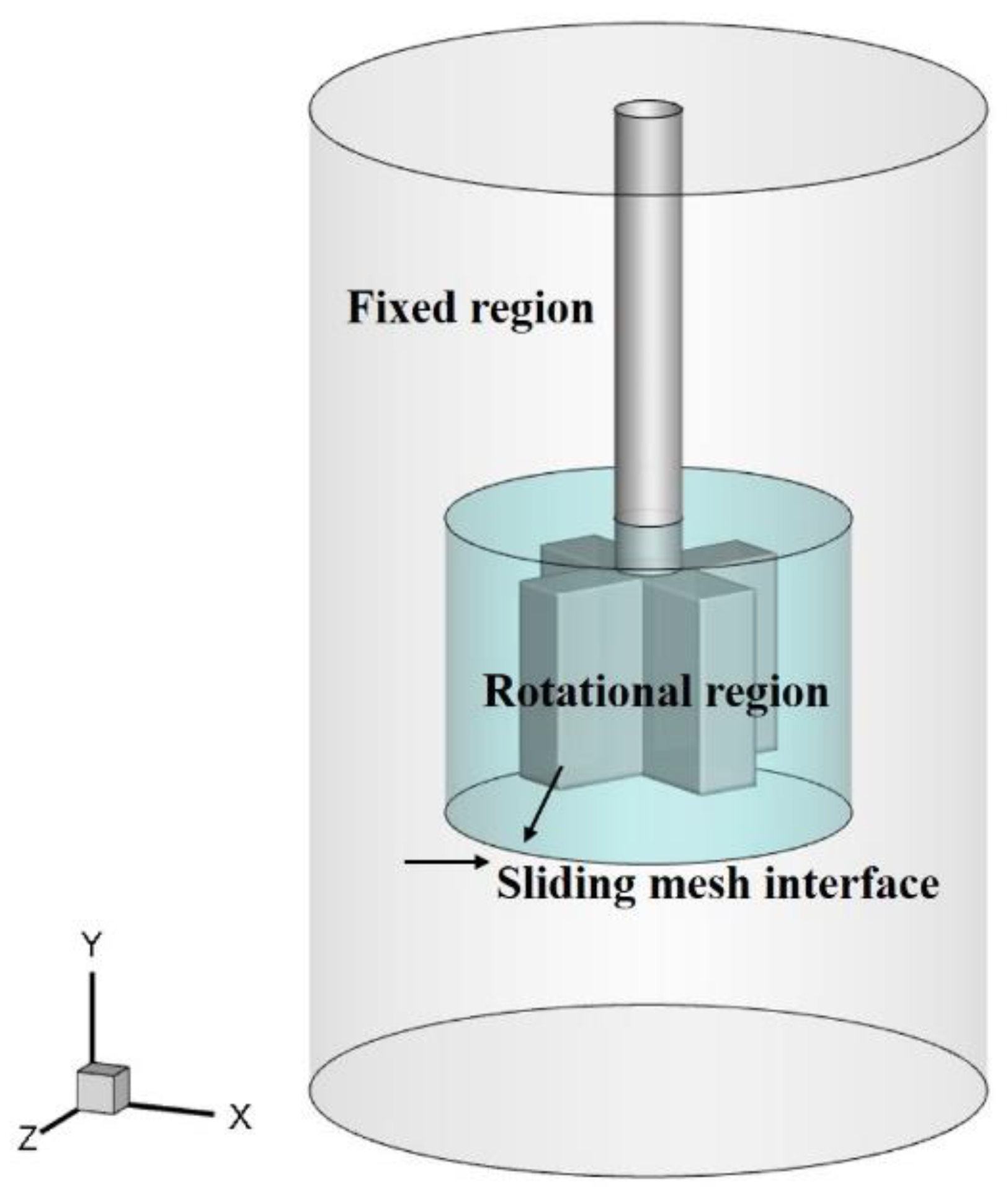
2.3. Sliding Mesh Method for Impeller Motion

The simulation of KRs involves the impeller motion, which requires specified numerical tactics. In the current study, the sliding mesh method (SMM) [24,25,26,27,28,29] is adapted, and full transient simulations are carried out using two grid zones (see Figure 1). Compared with other technologies used to numerically deal with the region motion, such as the multiple reference frame (MRF) method, there are no additional source terms inserted into the momentum equations, e.g., centrifugal, Coriolis, and Euler forces, but the mesh will be moving. In SMM, one grid zone (a rotational zone) is attached to the impeller to model the rotating motion during the mechanically stirred process. In contrast, the other grid zone is attached to the vessel wall (a fixed region), as shown in Figure 1. Since the nodes in the rotating region move rigidly in a given rotational zone for SMM, it is imperative that the interface between the zones consists of two overlapping faces, one of which is attached to the rotating region while the other is attached to the fixed region. Specifically, the sliding interface consists of a set of identical surface elements accessible from both sides of the interface. In a single movement step, the mesh in the moving region slides with a predefined velocity across the mesh in the fixed region. After each step, the interface vertices in the moving and static region will be reattached according to the initially computed vertex map list. The interaction between the two regions is modeled by interpolating the information across these interfaces. The SMM algorithm is used to allow for velocity and pressure data transfer from one domain to the other and vice versa.

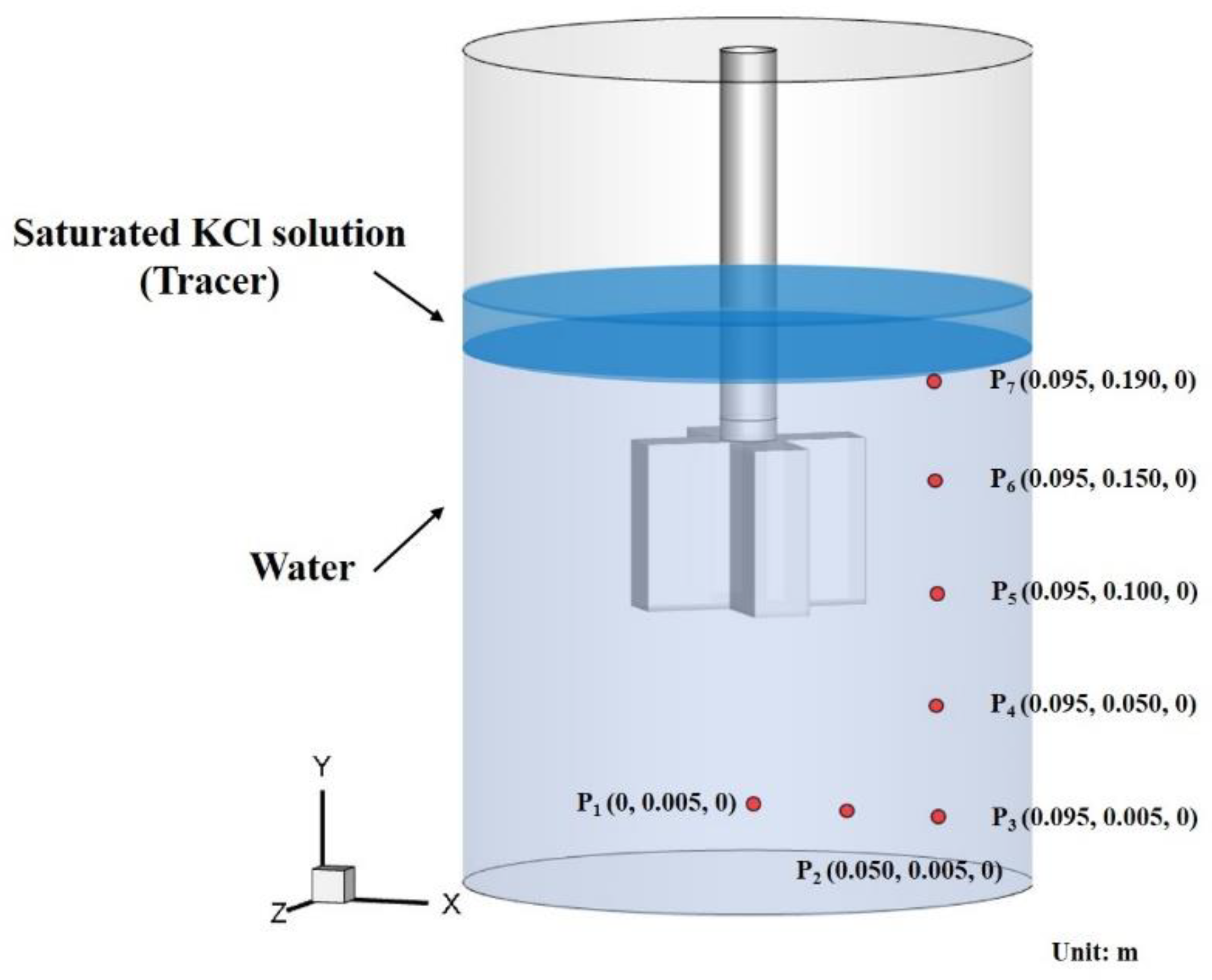
2.4. Tracer Transport Equation

To measure the mixing performance of KRs, the mixing time as a significant indicator has been adapted. Consequently, a passive scalar transport equation of the tracer, which is essentially governed by a convective–diffusion equation, has to be solved at each time step.

$$\rho \frac{\partial \left({\alpha }_{\mathrm{L}}C\right)}{\partial t}+\rho u_j\frac{\partial \left({\alpha }_{\mathrm{L}}C\right)}{\partial x_j}-\frac{\partial }{\partial x_j}\left[D_{\mathrm{eff}}\frac{\partial \left({\alpha }_{\mathrm{L}}C\right)}{\partial x_j}\right]=0$$

(14)

where C is the local tracer concentration, α_L is the liquid phase volume fraction, and D_eff is the effective diffusivity. The effective diffusion coefficient may be calculated as the sum of the molecular D_lam and turbulent diffusivities D_t. Here, D_lam is set as 10⁻⁹ m²/s, a typical value for a solute in liquids, and D_t is calculated from the turbulent kinetic viscosity ν_t as D_t = ν_t/Sc_t, where Sc_t is the turbulent Schmidt number and its value 0.7 is used. The velocity field used in the above tracer equation was obtained from a steady solution of VOF simulation and remained as a constant value during the calculation of this passive scalar.

The initial tracer concentrations are designated as zero everywhere in the vessel except at the blue Region A, as shown in Figure 2. To monitor the variation of tracer with time when measuring the mixing time, seven probe points were placed in several typical locations. Their coordinates are also listed in Figure 2.

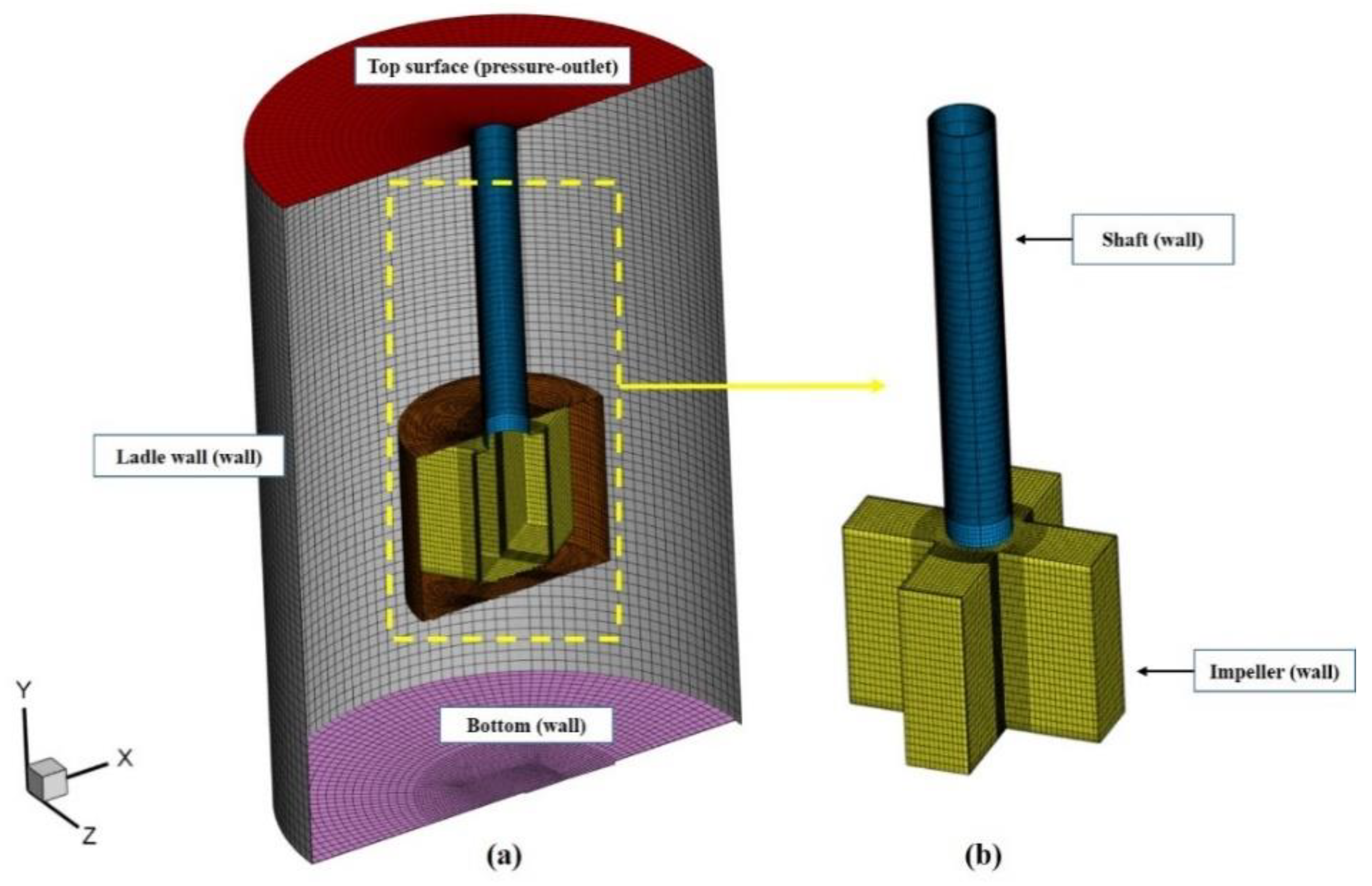
2.5. Computational Details and Boundary Conditions

A mesh with 450,000 cells, which is a reasonable balance between the computational cost (630,000 cells) and accuracy (260,000 cells), was used after the grid independence test in the previous research, which showed that the change of simulated results was <4% when further refining mesh. The typical mesh is shown in Figure 3. Figure 3a,b show the mesh details on the central vertical sections and the impeller.

As for boundary conditions in the current calculation, the top surface of the vessel is treated as a pressure outlet boundary, and the ladle wall, bottom, shaft, and impeller are treated as the no-slip wall boundary condition. The PISO algorithm is used to decouple the pressure–velocity. The discretization of the convective terms in the momentum and turbulence model equations employed the QUICK scheme, and the time step was set to 0.001 s. The calculations were carried out using the commercial computational fluid dynamic software FLUENT 14.5. The main convergence criterion is that the residuals for torque, velocity, and pressure achieve a steady state, i.e., they do not change significantly with further increasing time steps or iterations. The second criterion for checking the residuals was committed for all governing equations to less than 1 × 10⁻⁵. The detailed geometric and physical parameters in this study are shown in

Table 1. The geometrical, physical, and operating parameters used in this study.

Items	Values
Ladle diameter, D (mm)	200
Ladle height, H (mm) Blade length, d (mm) Blade height, h (mm) Blade thickness, w (mm) Impeller immersion depth, I (mm) Impeller rotation speed, ω (rpm) Height filled with liquid water, H2 (mm) Water density, ρs (kg/m3) Water dynamic viscosity, μs (Pa·s) Top air density, ρo (kg/m3) Top air dynamic viscosity, μo (Pa·s) Total mesh number (-)	300 80 60 20 100, 110, 120, 130 180, 200, 220, 240, 260 200 998.2 0.001 1.225 1.79 × 10−5 ~450,000

.

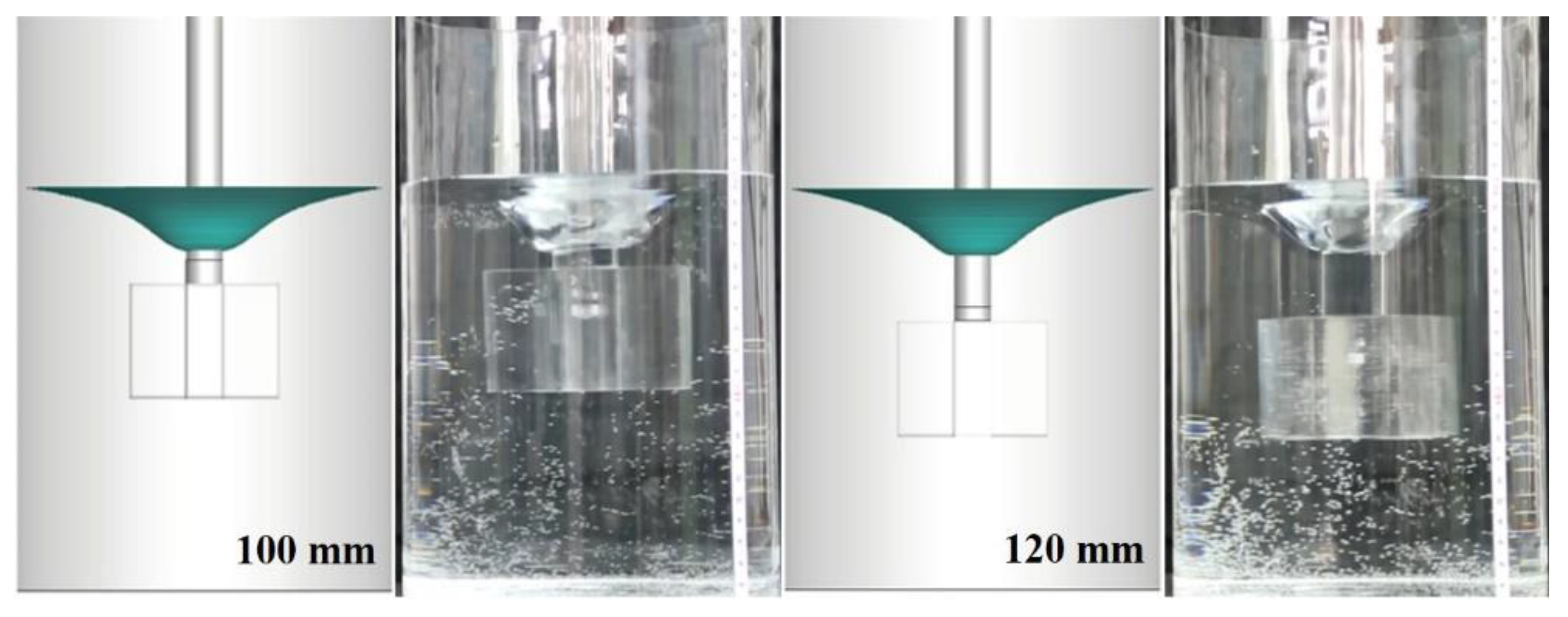
2.6. Model Validation

Model validations have been reported [20]. Because the availability of the industrial KR process data is limited by the measurement technology and the high costs of in-situ experimentation due to a high temperature under hazardous conditions, the water model experiments were resorted to in order to validate the model. Here, similar conditions of the water model for KR have been adapted. In earlier studies, the effect of the impeller dimension on the fluid flow and interface behavior was investigated based on numerical simulation. It was found that the flow field and interface behavior of the process of KR hot metal pretreatment can be represented by a 3D Volume of Fluid (VOF) model coupling the sliding mesh method and RNG k-ε model. The water model experiment was designed to validate the present mathematical model. The simulated results based on the current model are in good agreement with the measured results in the water model, which corroborates the applicability of the proposed model.

Furthermore, concerning the rotational speed and immersion depth, the comparison of the vortex profile between a water model and numerical simulation at the rotation velocity of 180 rpm and different impeller immersion depths is shown in Figure 4. Figure 5 shows the vortex depth of the water model and the numerical simulation at the impeller immersion depth of 110 mm with different rotation speeds. It is observed that the shape and vortex depth can be well captured, and specific agreement between the simulated and experimental results can reasonably arrive.

3. Results and Discussion

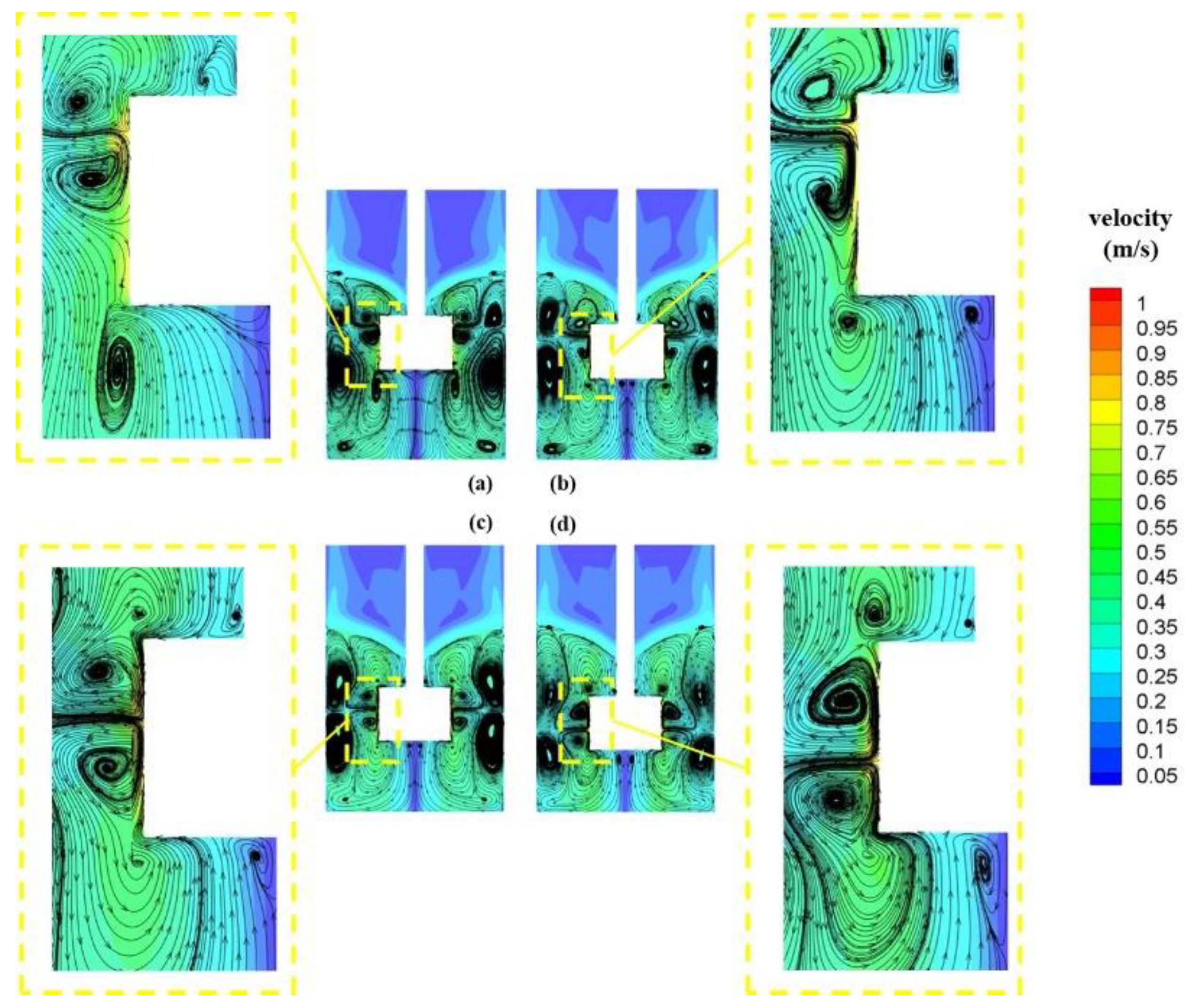
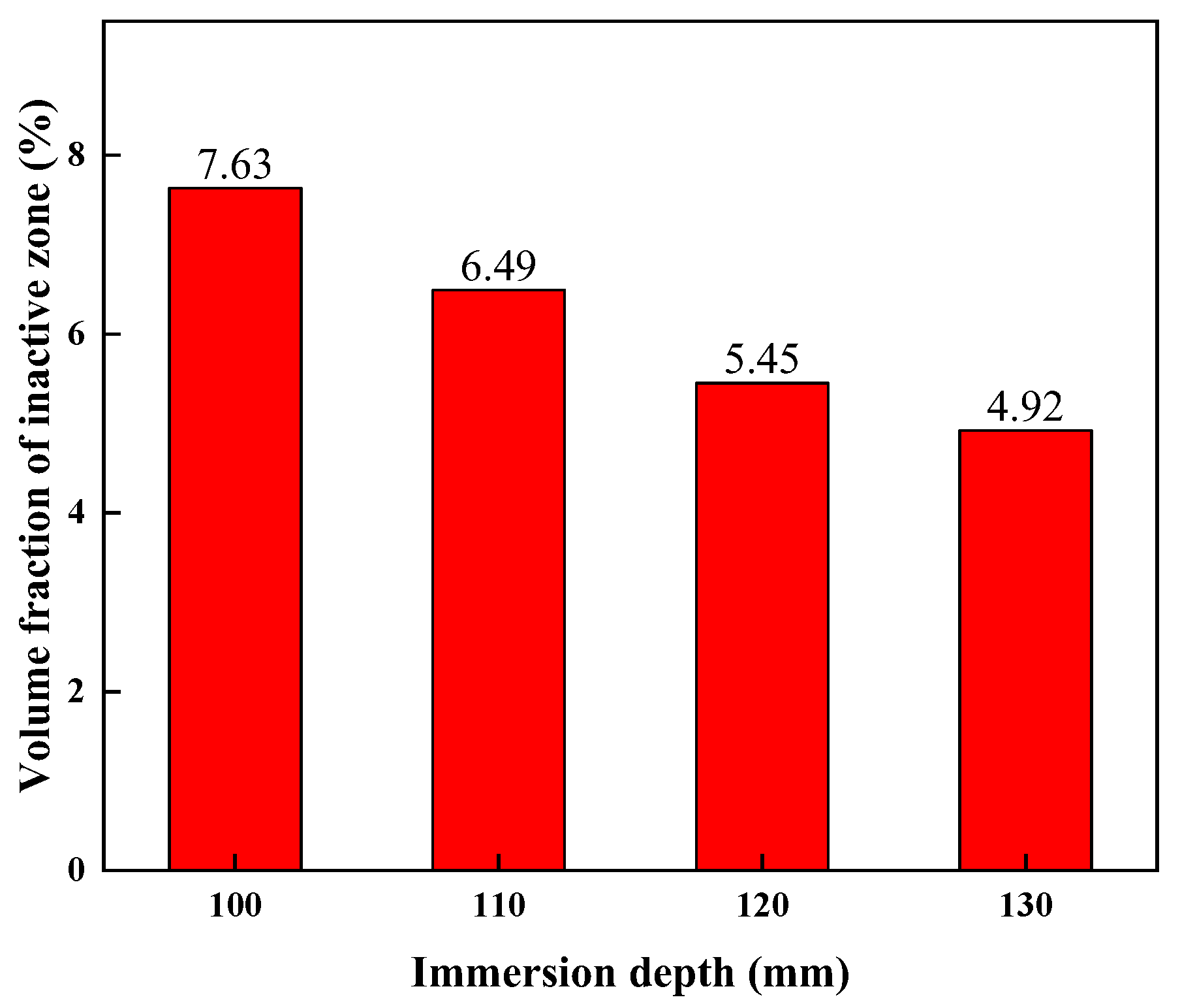
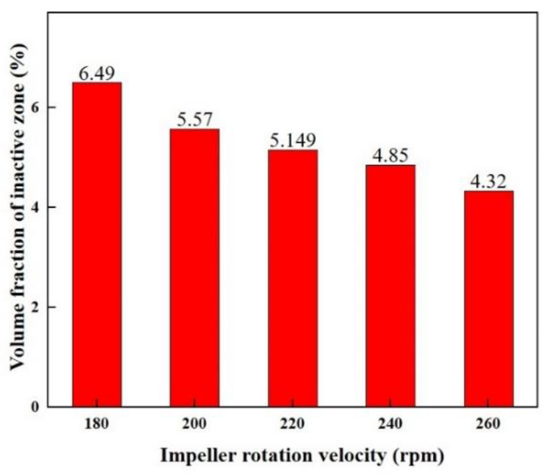
3.1. Fluid Flow Pattern and Qualifying Inactive Zone

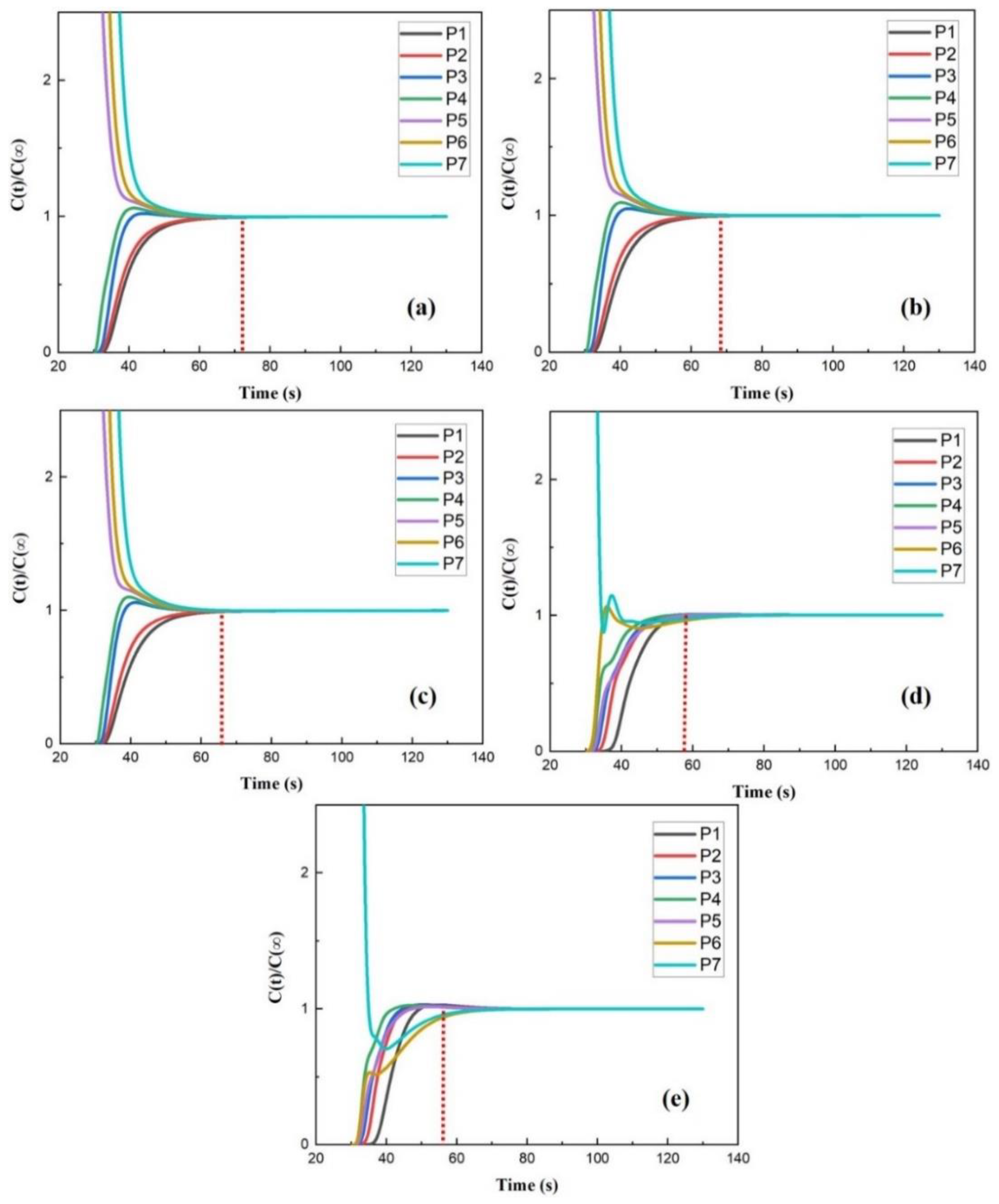
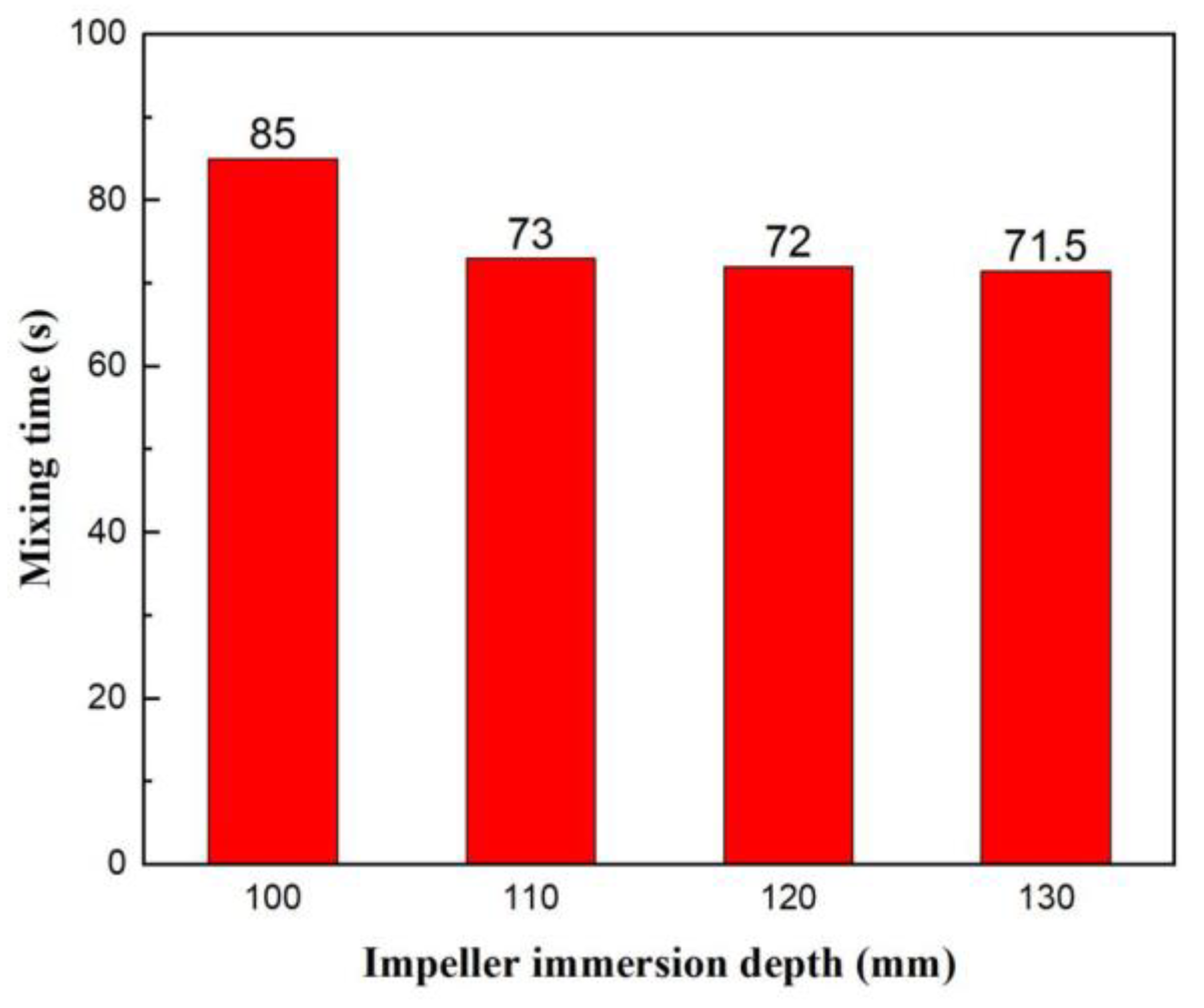
The bath flow in KRs is driven by the high-speed rotating impeller, which directly transfers kinetic energy to the liquid and mixes it with reagent powders for desulfurization. Consequently, it is worth investigating the effect of impeller immersion depth (IID) and impeller rotation speed (IRS) on the stirring and mixing characteristic of KRs. Figure 6 shows the central vertical cross-section streamlines and a close-view of the local region around the impeller at an immersion depth of 100 mm, 110 mm, 120 mm, and 130 mm. The simulation conditions can be found in Table 1, and here the rotation speed of the impeller is fixed to 180 rpm. Similar to our previous study, two main recirculation flow patterns, where the flow field is separated into the upper and lower zones by the discharge flow driven by the impeller rotation, were also observed in Figure 6. With the increase of the impeller immersion depth, the root location of discharge flow moves downward, but the discharge strength, i.e., the maximum velocity, appears to remain invariant for all cases; see the corresponding close-view of the local region around the impeller in Figure 6a–d. As a result, the upper recirculation zone was expanded. This flow pattern change would influence the local and global mixing characteristics.

In contrast, the flow pattern under different IRSs is also shown in Figure 7a–e, which gives the vertical cross-section flow field and streamlines at IRSs of 180 rpm, 200 rpm, 220 rpm, 240 rpm, and 260 rpm. Flow velocity in the bath, both local and global, has been increased significantly with the increase of IRS. However, the root location of discharge flow with increasing IRS shows almost no change. These results reveal that the effects of IRS and IID on the flow pattern are different. These results also make it possible to operationally control the flow pattern in a KR via the complementarity of the two parameters.

Further, some quantities comparisons were also conducted. Figure 8a,b show the axial and radial velocity variations along Lines A and B. Line A is a vertical line of 0.075 m from the axial centerline of the vessel, and Line B is a horizontal line of 0.85 m from the bottom surface, which is illustrated in the subgraph of Figure 8a(1). Through comparison, it can be seen that the changing trend of velocities on Line A is the same. However, the level of maximum velocity decreases with the increase of IID, which can also be observed from the velocity contour of the central vertical section at different IIDs. Figure 8a(2) shows that the radial velocity distribution is almost axis-symmetrical. The velocity near the outside edge of the impeller is greater than at the center and near the wall. It can also be seen in Figure 8a(2) that the velocity along Line B below the impeller slightly increases when increasing IID, and the closer it is to the edge of the impeller, the more pronounced this increase is. Besides, the velocity below the impellers is always minimal, reaching almost zero. Finally, it should be stressed that the velocity change caused by the IID change is finite compared with the influence of IRS.

Figure 8b(1,2) show the axial and radial velocity variations at different IRSs. It can be observed that the axial and radial velocity increases significantly, and the diameter of the lower-velocity region decreases as the impeller rotation speed increases. However, for all the impeller rotation velocities, the velocity below the impeller is still miniscule, making it particularly difficult to achieve global mixing of the species in the reactor. Furthermore, Figure 9 shows the velocity distribution contour of horizontal sections with different heights under the different IRSs. It can be seen that the liquid velocity of different horizontal sections increases noticeably with increasing IRS. However, the velocity below the impeller is still very small no matter how fast the IRS is. These phenomena were also observed by T. Yamamoto et al. [7,8,9,10] in the flow characteristic of aluminum melt by mechanically stirring.

To further study the effect of operation parameters on the bath flow of KRs, the mean velocity of the fluid in the bath under different IIDs was also investigated by indirectly measuring the dynamic energy of the bath obtained from the mechanical stirring. Figure 10a shows the comparison of the mean velocities for different IIDs. As expected, when the immersion depth increases, the mean velocity is basically unchanged. The comparison of the mean velocity of the bath under different IRSs is shown in Figure 10b. The mean velocity increases linearly as the rotation speed increases but remains invariant when IID changes. The mean velocity of the liquid rises 0.022 m/s as the impeller rotation velocity increases by 10 rpm. Unlike related research, the relationship between the mean velocity of the bath and IRS has been further obtained. A fitting regression, where the mean velocity $\overline{v}$ is correlated with the impeller rotation speed ω, is calculated as follows:

$$\overline{v}=-0.0009+0.0022\omega \left(180\le \omega \le 260\right)R^2=0.9976$$

(15)

Additionally, to further examine the effect of IID and IRS on the volume fraction of the inactive zone, an indicator γ is defined, which is the ratio of the region size of flow velocity when it is less than 0.1 m/s to the fluid volume in the bath. The γ at different IIDs is shown in Figure 11. With the increase of IID, the γ decreased from 7.63% to 4.92%. Therefore, it can be inferred that the impeller immersion depth does significantly affect local mixing. A fitting regression of the volume fraction of the inactive zone γ as a function of impeller immersion depth I is obtained as follows.

$$\gamma =36.646-0.4425I+0.0015I^2\left(100\le I\le 130\right)R^2=0.9980$$

(16)

The volume fraction of the inactive zone at different rotation velocities is shown in Figure 12. The γ of the stirred molten pool decreases from 6.49% to 4.32% as the impeller rotation velocity increases from 180 rpm to 260 rpm. The γ decreases by 0.92% as the impeller rotation velocity increases from 180 rpm to 200 rpm, which is the maximum decline in the range of 180 rpm to 260 rpm. The γ drops linearly and monotonically in this range, i.e., the γ decreases by 0.2% as the impeller rotation velocity increases by 10 rpm. Further, a fitting regression of γ as a function of impeller rotation speed ω is obtained as follows:

$$\gamma =9.63-0.02\omega \left(200\le \omega \le 260\right)R^2=0.9889$$

(17)

3.2. Mixing Time

Mixing time is an essential index to measure mixing characteristics. In order to obtain the mixing time of the reactor, the stimulus–response method was used here. When simulations/experiments are fully developed, a certain amount of tracer, specifically, 50 mL of saturated KCl solution, is added to the reactor. The change of tracer concentration is recorded, and the mixing time defined as the time span from the moment the tracer is supplied to that when the concentration curves of all monitoring points approximate a constant value with a fluctuation range restricted to ±5 pct. Some related computational details are given in Section 2.4. Figure 13 plots the specific tracer concentration change at those monitoring points defined in Figure 2. Here, the response curves of tracer with time under different IRSs are shown in Figure 13a–e, which correspond to the IRSs of 180 rpm, 200 rpm, 220 rpm, 240 rpm, and 260 rpm, respectively. In Figure 13, the red vertical line indicates the mixing time based on the above definition. The curve of each point shows how to respond to the change of tracer concentrations and reveals the flow pattern to a certain extent. For example, monitoring point 7, the curves converge gradually on the equilibrium concentration for IRSs of 180, 200 and 220 rpm. Next, the curve has one peak for the IRS at 240 rpm. As the IRS increases to 260 rpm, the curves quickly converge on the equilibrium concentration; moreover, the period shortens with the rise of the IRS. Since the rotating impeller drives the fluid flows, the rotating velocity directly impacts the kinetic energy transferred to the fluid. Thus, with the increase of IRS, the response of the tracer to the fluid hydrodynamic becomes more and more intense, and the tracer concentration at each monitoring point arrives more quickly at the theoretical equilibrium concentration, which suggests the mixing should be reinforced significantly with increasing IRS.

Furthermore, the mixing time at different IRSs is shown in Figure 14. It decreases significantly with the increase of IRS. As can be seen from the above, with the increase of IRS, the mean velocity of the bath increases significantly. The minimum mixing time is 55 s for the IRS at 260 rpm—a maximum value in this study’s range. Meanwhile, the volume fraction of the inactive zone decreases visibly, which produces a decrease in mixing time. Consequently, the rise of the IRS is an effective means to shorten the mixing time.

The mixing time under different IIDs is shown in Figure 15. It can be seen that the variation trend of mixing time with IID is first reduced and then remains almost unchanged. The minimum mixing time is 71.5 s at an IID of 130 mm. Practically, when the IID range is between 110 mm and 130 mm, it always takes about 72 s to achieve global mixing. Obviously, IID has a limited impact on mixing time in this IID range. As is indicated above, with the increase of IID, the mean velocity of the bath has almost no change, but the volume fraction of the inactive zone decreases visibly. The volume fraction of the inactive zone at an IID of 100 mm is significantly greater than the other IIDs, making global mixing more difficult and increasing the mixing time. Consequently, compared with IID, IRS has a more significant effect on the mixing performance of the bath in KRs.

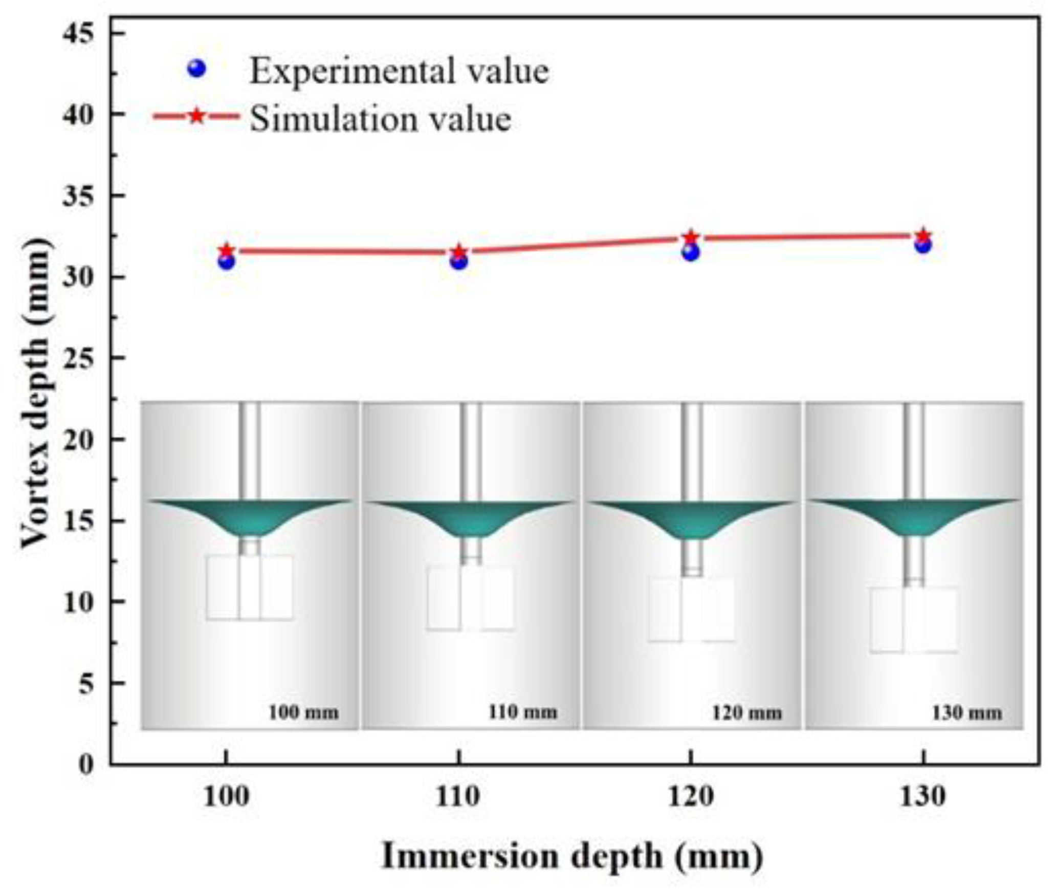
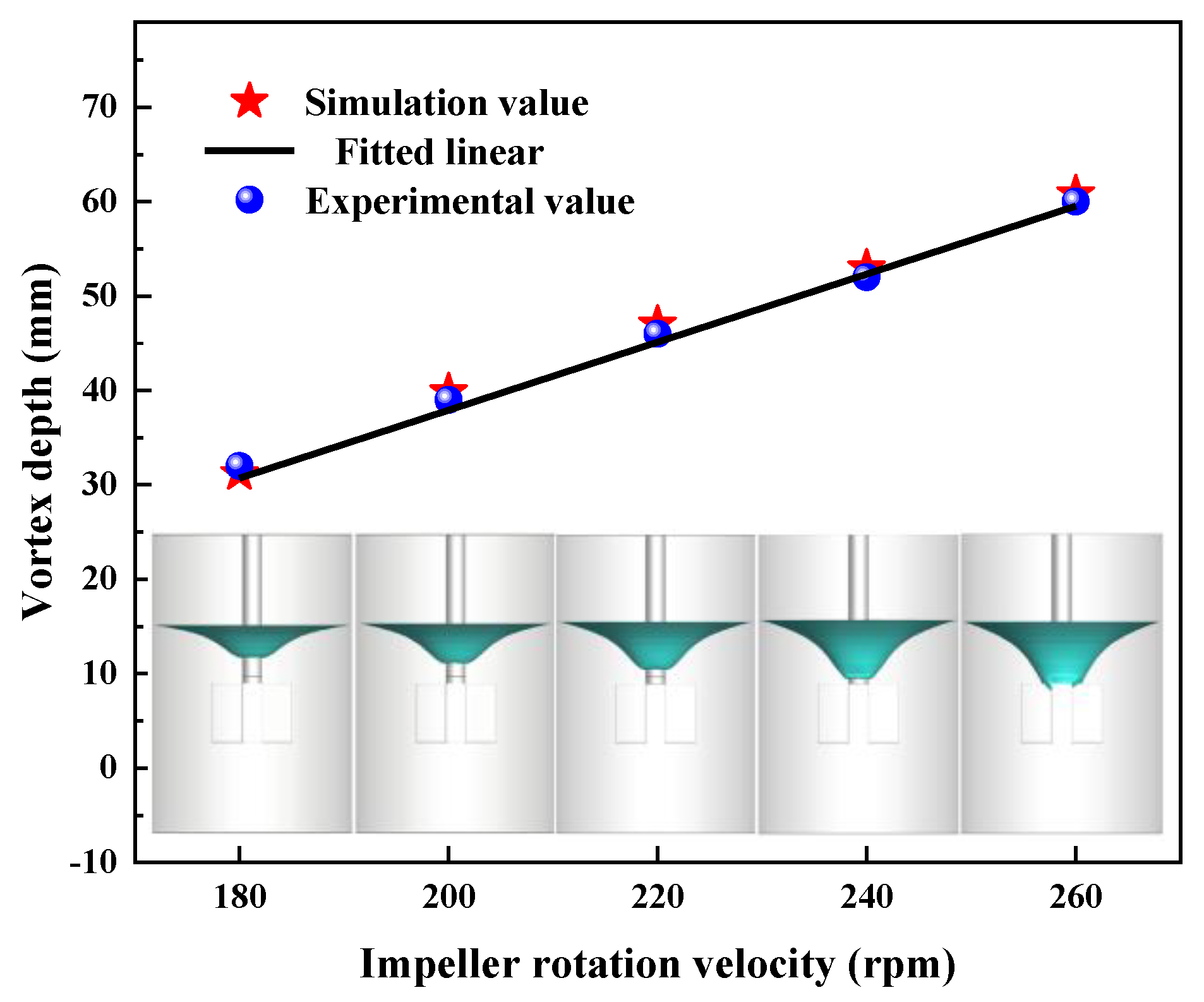
3.3. Vortex Core Depth

Vortex characteristics have an important influence on the dispersion behavior of particles and the refining efficiency, as reported in some studies [20]. It can be seen that there is almost no change to the profile of the gas–liquid interface and vortex core depth at different impeller immersion depths, as shown in Figure 16. The distance between the bottom of the vortex core and the top edge of the impeller increases continuously as IID increases. However, this doesn’t mean that the immersion depth of the impeller does not affect the behavior of the gas–liquid interface; this is discussed further in Section 3.4.

Increasing rotation speed is an effective way to increase the vertex core depth (VCH), favoring the entrainment and dispersion of the reagent by an impeller. The vortex depth and gas–liquid interface profile under different rotation speeds are shown in Figure 17. This figure vividly depicts how impeller rotation speed strongly impacts the vortex core depth and gas–liquid interface profile. The vortex core depth gradually increases as the IRS increases. Until reaching a rotation speed of 260 rpm, the bottom of the vortex passes the upper interface of the impeller, which is advantageous to the dispersion behavior of particles and the refining efficiency. The results of the vortex core depth with respect to the numerical simulation and water model experiment under different rotation speeds were also plotted in Figure 17. T. Yamamoto et al. [7,8] have reported the morphological changes to a free surface with different IRSs. The present work further analyses the relationship between the vortex depth and impeller rotation speed. To further investigate the effect of IID and IRS on the interfacial behavior of KRs, the free surface velocity is reported in Section 3.4. A fitting regression of the vortex core depth H_VCD as a function of impeller rotation speed ω is obtained as follows.

$$H_{\mathrm{VCD}}=-33.25+0.36\omega \left(180\le \omega \le 260\right)R^2=0.9965$$

(18)

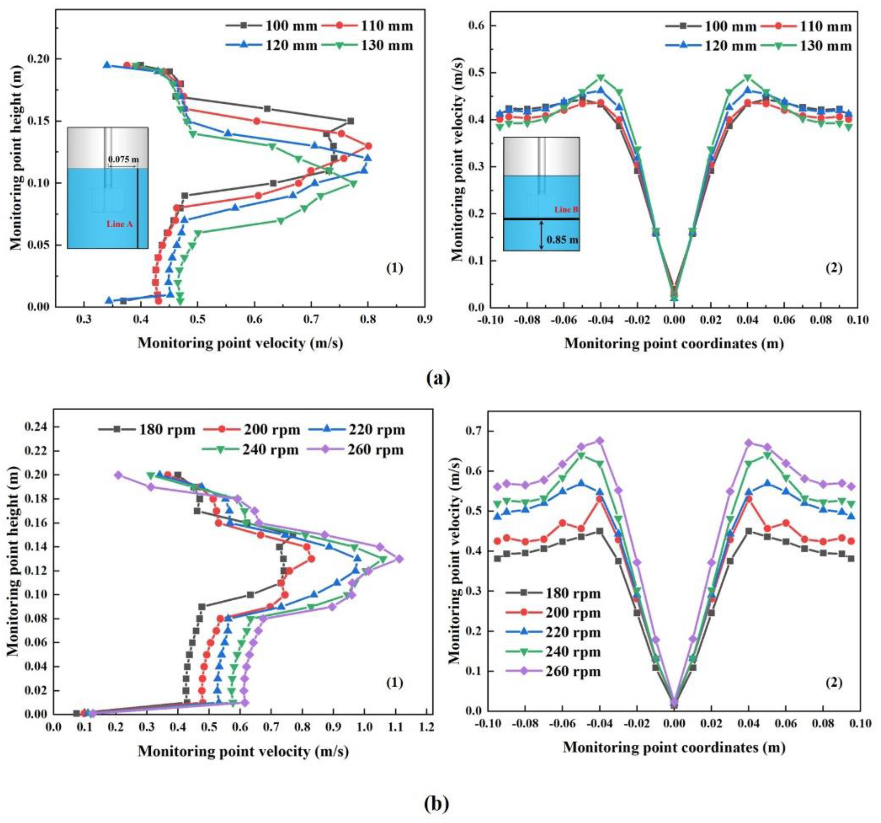
3.4. Free Surface Velocity

The velocity on the gas–liquid interface strongly influences the entrainment and entrapment of the desulfurization particles. The interface velocity at different IIDs is shown in Figure 18. It clearly indicates that the velocity around the vortex core is much bigger than that near the walls, i.e., there is a gradient of velocity along the radial direction. It also suggests that the regents around the vortex core are much more active than those near the walls. Furthermore, with the increase of IID, the distance between the bottom of the vortex core and impeller increases, resulting in the rotational impeller’s effect on the interface velocity around the bottom of the vortex core being less pronounced. Consequently, the velocity gradient between the axis–centerline and walls becomes insignificant when the impeller is taken down. For example, the velocity on the gas–liquid interface around the vortex core is obviously greater than those near the walls for immersion depths of 100 mm, i.e., the change of interface velocity along with radial direction is relatively steep for the small IID (see Figure 18a). However, for the case of IID at 130 mm, the change of velocity, along with radial direction, is relatively even (see Figure 18d). As a result, the interface velocity near the vortex core decreases significantly with the increasing IID, which reveals that the entrainment and dispersion effect of the vortex is affected by the arrangement of IID.

In addition, the velocity distribution on the gas–liquid interface at different IRSs was investigated, and the simulation results are shown in Figure 19. The velocity on the gas–liquid interface increases significantly with the rise of IRS; this phenomenon can be explained in terms of a high-speed rotating impeller that intensely powers the velocity of the gas–liquid interface. Notably, for the case of IRS at 260 rpm, the bottom of the vortex core sunk below the top edge of the impeller. Thus, it makes the interface velocity near the impeller sharply increase and dramatically promotes the dispersion behavior of the reagents and desulfurization efficiency.

4. Conclusions

Based on the developed 3D VOF-SMM model, the influences of operating parameters on bath flow, mixing characteristics, and interface behaviors for KR process are numerically investigated and arrive at the following results:

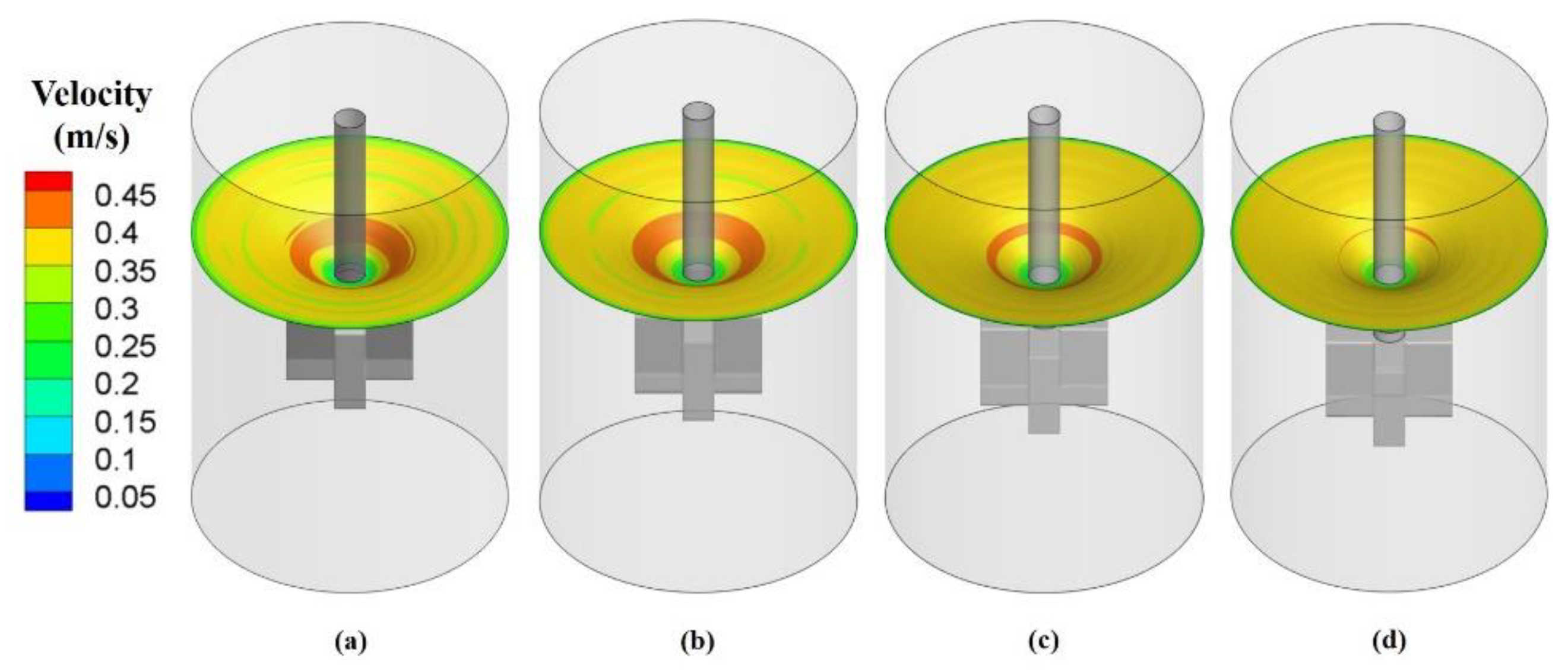
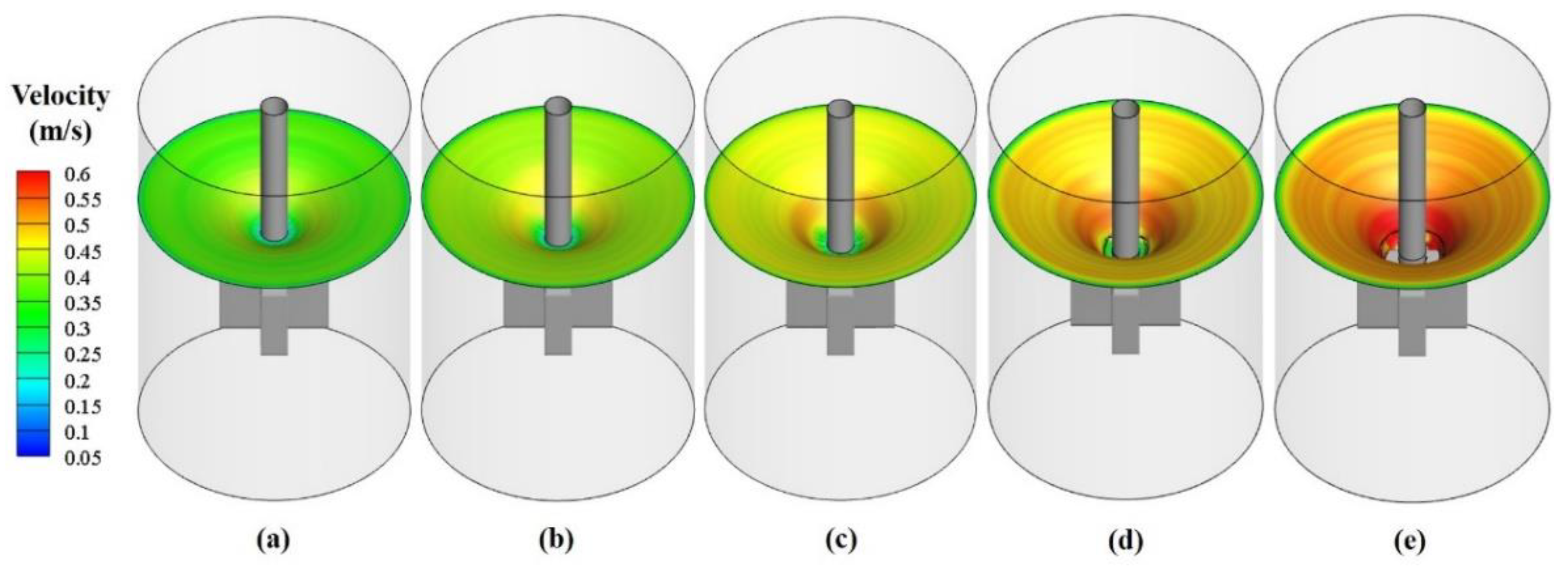
• Impeller immersion depth and rotation speed have different effects on the fluid flow pattern of the bath under the present study range. The root location of the discharge flow moves downward with the impeller immersion depth increasing, but the discharge strength and the mean velocity of the bath show hardly any change. Comparatively, the increase in the impeller rotation speed significantly improves the mean velocity, but there is little change in the position of discharge flow. Furthermore, increasing impeller immersion depth or rotation speed can effectively reduce the volume fraction of the inactive zone, but it cannot eliminate it. As a result, the correlation equations of γ as a function of ω or I are formulated under the range of $180\le \omega \le 260$ and $100\le I\le 130$, respectively.
• Increasing impeller rotation speed is the most direct and effective way to shorten the mixing time. However, the impeller immersion depth has a limited impact on the mixing time by comparison. In the present study, a minimum mixing time of 55 s is achieved at the maximum impeller rotation speed of 260 rpm.
• The vortex core depth and the velocity at the gas–liquid interface increase significantly with the increasing impeller rotation speed, and a linear fitting regression has been proposed. However, while the impeller immersion depth has little effect on the vortex core depth, it has a visible influence on the velocity distribution of the free surface. The velocity gradient on the gas–liquid interface between the axis to walls becomes steep with the decreasing impeller immersion depth.

References

1. Visuri, V.-V.; Vuolio, T.; Haas, T.; Fabritius, T. A Review of Modeling Hot Metal Desulfurization. Steel Res. Int. 2020, 91, 1–25. [Google Scholar] [CrossRef] [Green Version]
2. Schrama, F.N.H.; Beunder, E.M.; Berg, B.V.D.; Yang, Y.; Boom, R. Sulphur removal in ironmaking and oxygen steelmaking. Ironmak. Steelmak. 2017, 44, 333–343. [Google Scholar] [CrossRef]
3. Kanbara, K.; Nisugi, S.; Shiraishi, O.; Katakeyama, T. Desulfurization approach with mechanically stirred. Tetsu-To-Hagané 1972, 58, S26–S34. [Google Scholar]
4. Nakai, Y.; Sumi, I.; Kikuchi, N.; Tanaka, K.; Miki, Y. Powder Blasting in Hot Metal Desulfurization by Mechanical Stirring Process. ISIJ Int. 2017, 57, 1029–1036. [Google Scholar] [CrossRef] [Green Version]
5. Wang, Q.; Jia, S.; Tan, F.; Li, G.; Ouyang, D.; Zhu, S.; Sun, W.; He, Z. Numerical Study on Desulfurization Behavior during Kanbara Reactor Hot Metal Treatment. Metall. Mater. Trans. B. 2021, 52, 1085–1094. [Google Scholar] [CrossRef]
6. Shao, P.; Zhang, T.; Liu, Y.; Zhao, H.; He, J. Numerical Simulation on Fluid Flow in Hot Metal Pretreatment. J. Iron Steel Res. Int. 2011, 18, 129–134. [Google Scholar]
7. Yamamoto, T.; Kato, W.; Komarov, S.V.; Ishiwata, Y. Investigation on the Surface Vortex Formation during Mechanical Stirring with an Axial-Flow Impeller Used in an Aluminum Process. Met. Mater. Trans. A 2019, 50, 2547–2556. [Google Scholar] [CrossRef]
8. Yamamoto, T.; Fang, Y.; Komarov, S.V. Surface vortex formation and free surface deformation in an unbaffled vessel stirred by on-axis and eccentric impellers. Chem. Eng. J. 2019, 367, 25–36. [Google Scholar] [CrossRef]
9. Kato, K.; Yamamoto, T.; Komarov, S.V.; Taniguchi, R.; Ishiwata, Y. Evaluation of Mass Transfer in an Aluminum Melting Furnace Stirred Mechanically during Flux Treatment. Mater. Trans. 2019, 60, 2008–2015. [Google Scholar] [CrossRef] [Green Version]
10. Komarov, S.; Yamamoto, T.; Arai, H. Incorporation of Powder Particles into an Impeller-Stirred Liquid Bath through Vortex Formation. Materials 2021, 14, 2710. [Google Scholar] [CrossRef]
11. He, M.; Wang, N.; Hou, Q.; Chen, M.; Yu, H. Coalescence and sedimentation of liquid iron droplets during smelting reduction of converter slag with mechanical stirring. Powder Technol. 2020, 362, 550–558. [Google Scholar] [CrossRef]
12. He, M.; Wang, N.; Chen, M.; Li, C. Distribution and motion behavior of desulfurizer particles in hot metal with mechanical stirring. Powder Technol. 2020, 361, 455–461. [Google Scholar] [CrossRef]
13. Li, M.; Tan, Y.; Sun, J.; Xie, D.; Liu, Z. Drawdown mechanism of light particles in baffled stirred tank for the KR desulphurization process. Chin. J. Chem. Eng. 2019, 27, 247–256. [Google Scholar] [CrossRef]
14. Li, M.; Tan, Y.; Liu, Y.; Sun, J.; Xie, D.; Liu, Z. Effects of geometrical and physical factors on light particles dispersion by agitation characteristic curve. Chin. J. Chem. Eng. 2019, 27, 2313–2324. [Google Scholar] [CrossRef]
15. Nakai, Y.; Sumi, I.; Matsuno, H.; Kikuchi, N.; Kishimoto, Y. Effect of Flux Dispersion Behavior on Desulfurization of Hot Metal. ISIJ Int. 2010, 50, 403–410. [Google Scholar] [CrossRef] [Green Version]
16. Nakai, Y.; Hino, Y.; Sumi, I.; Kikuchi, N.; Uchida, Y.; Miki, Y. Effect of Flux Addition Method on Hot Metal Desulfurization by Mechanical Stirring Process. ISIJ Int. 2015, 55, 1398–1407. [Google Scholar] [CrossRef] [Green Version]
17. Ji, J.-H.; Liang, R.-Q.; He, J.-C. Simulation on Mixing Behavior of Desulfurizer and High-sulfur Hot Metal Based on Variable-velocity Stirring. ISIJ Int. 2016, 56, 794–802. [Google Scholar] [CrossRef] [Green Version]
18. Sahu, M.K.; Sahu, R.K. Optimization of Stirring Parameters Using CFD Simulations for HAMCs Synthesis by Stir Casting Process. Trans. Indian Inst. Met. 2017, 70, 2563–2570. [Google Scholar] [CrossRef]
19. Liu, Y.; Zhang, T.-A.; Sano, M.; Wang, Q.; Ren, X.-D.; He, J.-C. Mechanical stirring for highly efficient gas injection refining. Trans. Nonferrous Met. Soc. China 2011, 21, 1896–1904. [Google Scholar] [CrossRef]
20. Li, Q.; Shen, X.; Guo, S.; Li, M.; Zou, Z. Computational Investigation on Effect of Impeller Dimension on Fluid Flow and Interface Behavior for Kanbara Reactor Hot Metal Treatment. Steel Res. Int. 2021, 92, 1–15. [Google Scholar] [CrossRef]
21. Li, M.; Shao, L.; Li, Q.; Zou, Z. A Numerical Study on Blowing Characteristics of a Dynamic Free Oxygen Lance Converter for Hot Metal Dephosphorization Technology Using a Coupled VOF-SMM Method. Met. Mater. Trans. A 2021, 52, 1–12. [Google Scholar] [CrossRef]
22. Ubbink, O.; Issa, R. A Method for Capturing Sharp Fluid Interfaces on Arbitrary Meshes. J. Comput. Phys. 1999, 153, 26–50. [Google Scholar] [CrossRef] [Green Version]
23. Hirt, C.W.; Nichols, B.D. Volume of fluid (VOF) method for the dynamics of free boundaries. J. Comput. Phys. 1981, 39, 201–225. [Google Scholar] [CrossRef]
24. Chuprov, P.; Utkin, P.; Fortova, S. Numerical Simulation of a High-Speed Impact of Metal Plates Using a Three-Fluid Model. Metals 2021, 11, 1233. [Google Scholar] [CrossRef]
25. Wang, Y.; Cao, L.; Cheng, Z.; Blanpain, B.; Guo, M. Mathematical Methodology and Metallurgical Application of Turbulence Modelling: A Review. Metals 2021, 11, 1297. [Google Scholar] [CrossRef]
26. Luo, J.Y.; Gosman, A.D.; Issa, R.I.; Middleton, J.C.; Fitzgerald, M.K. Full flow field computation of mixing in baffled stirred vessels. Chem. Eng. Res. Des. 1993, 71, 342–344. [Google Scholar]
27. Torotwa, I.; Ji, C. A Study of the Mixing Performance of Different Impeller Designs in Stirred Vessels Using Computational Fluid Dynamics. Designs 2018, 2, 10. [Google Scholar] [CrossRef] [Green Version]
28. Tanaka, R.; Uddin, A.; Kato, Y. Flow Characteristics Related to Liquid/liquid Mixing Pattern in an Impeller-stirred Vessel. ISIJ Int. 2018, 58, 620–626. [Google Scholar] [CrossRef] [Green Version]
29. Wang, Q.; Liu, Y.; Cao, Y.; Li, G. Study on Sulfur Transfer Behavior during Refining of Rejected Electrolytic Manganese Metal. Metals 2019, 9, 751. [Google Scholar] [CrossRef] [Green Version]
Figure 1. The computational domain consisted of the fixed and rotational regions and separated the sliding mesh interface.
Metals 11 01596 g001
Figure 2. Schematic illustration of tracer addition region and the position of monitoring points with detailed coordinates.
Metals 11 01596 g002
Figure 3. Numerical mesh of (a) central vertical profiles and (b) impeller.
Metals 11 01596 g003
Figure 4. Comparison of vortex depth of numerical simulation and water model at impeller immersion depths of 100 mm and 120 mm.
Metals 11 01596 g004
Figure 5. Comparison of vortex depth of numerical simulation and water model at impeller rotation velocities of 220 rpm and 260 rpm.
Metals 11 01596 g005
Figure 6. The streamlines of the central vertical cross-section at an immersion depth of (a) 100 mm, (b) 110 mm, (c) 120 mm, and (d) 130 mm.
Metals 11 01596 g006
Figure 7. The flow field and streamlines of the central vertical cross-section at impeller rotation speeds (IRSs) of (a) 180 rpm, (b) 200 rpm, (c) 220 rpm, (d) 240 rpm, and (e) 260 rpm.
Metals 11 01596 g007
Figure 8. Comparison of velocity distributions along with Line A for the axial direction in sub-graph (1) and Line B for the radial direction in sub-graph (2) at different (a) IIDs and (b) IRSs.
Metals 11 01596 g008
Figure 9. The velocity distribution of different levels at IRS of (a) 180 rpm, (b) 200 rpm, (c) 220 rpm, (d) 240 rpm and (e) 260 rpm.
Metals 11 01596 g009
Figure 10. Comparison of the mean velocities of the fluid in the bath at different (a) impeller immersion depths (IIDs) and (b) IRSs.
Metals 11 01596 g010
Figure 11. Comparison of the volume fraction of inactive zones at different IIDs.
Metals 11 01596 g011
Figure 12. Variation of the volume fraction of the inactive zones at different IRSs.
Metals 11 01596 g012
Figure 13. The change of tracer concentration of monitoring points with time at IRS of (a) 180 rpm, (b) 200 rpm, (c) 220 rpm, (d) 240 rpm, and (e) 260 rpm.
Metals 11 01596 g013
Figure 14. Comparison of mixing times at different IRSs.
Metals 11 01596 g014
Figure 15. Comparison of mixing times at different IIDs.
Metals 11 01596 g015
Figure 16. Vortex depth and gas–liquid interface profile at different IIDs with IRSs of 180 rpm.
Metals 11 01596 g016
Figure 17. Vortex depth and gas–liquid interface profile at different IRSs with IIDs of 110 mm.
Metals 11 01596 g017
Figure 18. Comparison of gas–liquid interface velocity at different IIDs of (a) 100 mm, (b) 110 mm, (c) 120 mm and (d) 130 mm.
Metals 11 01596 g018
Figure 19. Comparison of gas–liquid interface velocity at different IRSs at (a) 180 rpm, (b) 200 rpm, (c) 220 rpm, (d) 240 rpm, and (e) 260 rpm.
Metals 11 01596 g019