Molten Pool Behaviors in Double-Sided Pulsed GMAW of T-Joint: A Numerical Study

Abstract

The T-joint is one of the essential types of joints in aluminum welded structures. Double-sided welding is a preferable solution to maintain high efficiency and avoid significant distortion during T-joint welding. However, interactions between double-sided molten pools make flow behaviors complicated during welding. Numerical simulations regarding molten pool behaviors were conducted in this research to understand the complex flow phenomenon. The influences of wire feed rates and torch distances were simulated and discussed. The results show that droplet impinging drives the fluid to flow down to the root and form a frontward vortex. Marangoni stress forces the fluid to form an outward vortex near the molten pool boundary and flatten the concave-shaped molten pool surface. With an increased wire feed speed, the volume of the molten pool increases, and the root fusion is improved. With an increased torch distance, the width of the front molten pool decreases while the length increases, and the rear molten pool size decreases slightly. Both wire feed speeds and the torch distances have limited influences on the basic flow characteristics.

1. Introduction

Aluminum alloys are widely used in engineering structures due to their excellent specific strength and corrosion resistance. Welding is one of the essential processing techniques used to fabricate heavy aluminum alloy structures. For welded aluminum structures, the T-joint is one of the essential types of joints. In this joint, a vertical plate is joined with a horizontal plate using two symmetrical weld beads. This characteristic determines that double-sided welding is a preferable solution to maintain high efficiency and avoid significant distortion. However, during double-sided welding, interactions between double-sided molten pools are complicated, especially when the amount of penetration is large. Thus, the welding quality is usually hard to control in real-world welding practice. Although, the weld quality can be improved via the hybridization method as Prajapati et al. proved [1,2]. However, for double-sided welding, the welding parameters are much more complicated than those in single-sided welding to coordinate the two electric arcs. Optimizing the welding process via experiments is time-consuming.

Fortunately, computer-aided engineering (CAE)-guided welding process optimization can be a promising alternative, which has recently attracted worldwide attention [3]. Numerical simulations have been proved in different welding conditions to be able to visualize and forecast the multiscale welding physical phenomenon [4] and even establish the relationship between process and mechanical properties [5]. Optimization methods for numerical models with finite experiments are also proposed to improve the simulation precision [6]. However, for T-joint welding, reported numerical research currently only focuses on residual stress analysis, distortion control, and reliability analysis. Chang et al. [7] and Luca et al. [8] explored the residual stress distribution of T-joints made of dissimilar steels. Zhang et al. [9] and Khoshroyan et al. [10] investigated the influences of welding parameters on residual stress and distortions. Deng et al. simulated the control effects of optimizing weld bead arrangement, weld sequence [11], and fixtures [12] on residual distortion. Chu et al. [13] simulated the possibility of introducing compressive residual stress into T-joints via overlay welding. High-efficiency simulation methods were proposed based on the shell/3D technique [14], heat source simplification [15], and the inherent strain method [16]. Structural behaviors of T-joints under different loading conditions [17,18,19,20] were simulated, and the influences of welding defects were considered with modern modeling software [21].

In all these studies, the fluid flow in molten pools was ignored. However, as an essential welding phenomenon, the molten pool is the key factor influencing the welding appearance, metallurgical reactions, penetrations, defects formation, and finally, the welding quality. A deep understanding of molten pool behavior during welding is helpful and necessary for designing process parameters.

Numerical simulations of molten pools in arc welding have been investigated for more than 30 years. Kou et al. [22] conducted one of the early studies on stationary tungsten inert gas (TIG) welding in 1985. After that, two research hotspots gradually formed. One was the model improvement for different welding conditions or higher precision. Cho et al. [23] proposed a force model for V-groove gas tungsten arc (GTA) and gas metal arc (GMA) welding. Then, they developed asymmetric heat sources for second-pass GMA welding [24]. Bahrami et al. [25] developed a model considering the mass transfer to simulate the welding of dissimilar materials. Jeong et al. [26] proposed a separate heat source to simulate the molten pool flow in lap joint GTA welding. Hao et al. [27] proposed a similar model to simulate TIG welding with a reserved gap. Cho et al. [28] discussed the model setups for more realistic modeling results of one pulse one drop GMA welding. Full coupled numerical models to simultaneously simulate the electric, droplet, and molten pool were also proposed [29,30]. However, the conditions are usually 2D and stationary due to the limitation of computation efficiency.

Using molten pool simulation to visualize the intrinsic mechanism of the welding phenomenon and optimizing the welding process based on that is the other hotspot. Traidia et al. [31] explored the formation mechanism of asymmetric bead appearance during horizontal narrow-gap TIG welding. Liu et al. [32] investigated the formation process of ripples in pulsed GTA welding. Cheon et al. [33] discussed the cause of finger-shaped penetration in GMA welding. Meng et al. and Pan et al. investigated the origin of humping [34,35] and undercut [35] defects during GTA welding. Then, the influencing mechanisms of vibration [36], double electrode [37], ultrasonic waves [38], magnetic fields [39], and gravity [40] on the molten pool flow were simulated and visualized. With the understanding of the complex flow behaviors in various conditions established, predicting or optimizing the welding process also becomes possible. Xu et al. [41] optimized the oscillating parameters in narrow-gap GMA welding via simulation. Additionally, Lang et al. [42] predicted the molten pool stability during variable polarity plasma arc welding (VPPAW).

Though significant progress has been made in previous studies, molten pool behavior during T-joint welding remains unclear, let alone in double-sided T-joint welding. In this study, to fill the knowledge gap, we developed a 3D numerical model to simulate the fluid flow during double-sided pulsed GMAW of aluminum T-joints. Then, the molten pool behaviors under different wire feed speeds and torch distances were visualized and investigated.

2. Numerical Model

2.1. Basic Assumptions

To make the complex physical phenomenon during double-sided GMA welding of the aluminum T-joint computable with acceptable precision and efficiency, we adopted the following assumptions:

(1)

The fluid flow in the weld pool is laminar, and the molted metal is incompressible.

(2)

The electric arc is not explicitly considered. Instead, the thermal and mechanical interactions between arcs and weld pools are considered by source terms.

(3)

The influences of metal vapor are ignored.

(4)

The physical and geometric heterogeneity of wire and base metal can be ignored.

(5)

The drop size and drop transfer frequency are assumed to be uniform.

2.2. Governing Equations

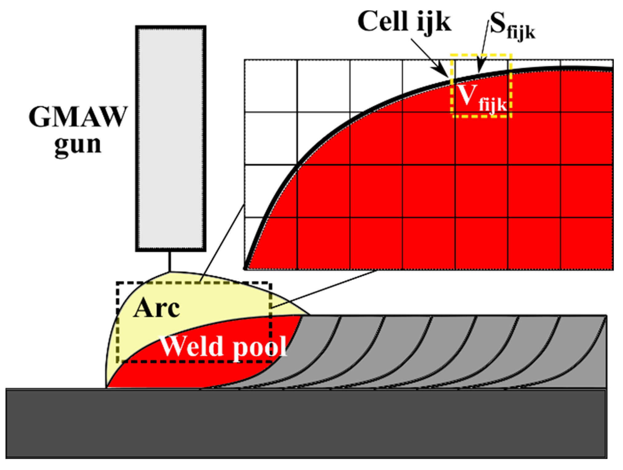
The following equations describe the fluid flow during the welding process with the above assumptions. Symbols and their physical meanings are described in the nomenclature table.

Mass continuity equation:

$$\frac{\partial \rho }{\partial t}+\frac{\partial (\rho u)}{\partial x}+\frac{\partial (\rho v)}{\partial y}+\frac{\partial (\rho w)}{\partial z}=S$$

(1)

where ρ is density, t is the time, u, v, and w are the velocity components in the x, y, and z directions, respectively, and S is the mass source (metal droplet in this work).

Momentum conservation equations:

$$\rho \left(\frac{\partial u}{\partial t}+u\frac{\partial u}{\partial x}+v\frac{\partial u}{\partial y}+w\frac{\partial u}{\partial z}\right)=-\frac{\partial p}{\partial x}+\mu \left(\frac{{\partial }^{2}u}{\partial x^2}+\frac{{\partial }^{2}u}{\partial y^2}+\frac{{\partial }^{2}u}{\partial z^2}\right)+F_{ex}$$

(2)

$$\rho \left(\frac{\partial v}{\partial t}+u\frac{\partial v}{\partial x}+v\frac{\partial v}{\partial y}+w\frac{\partial v}{\partial z}\right)=-\frac{\partial p}{\partial y}+\mu \left(\frac{{\partial }^{2}v}{\partial x^2}+\frac{{\partial }^{2}v}{\partial y^2}+\frac{{\partial }^{2}v}{\partial z^2}\right)+F_{ey}$$

(3)

$$\rho \left(\frac{\partial w}{\partial t}+u\frac{\partial w}{\partial x}+v\frac{\partial w}{\partial y}+w\frac{\partial w}{\partial z}\right)=-\frac{\partial p}{\partial z}+\mu \left(\frac{{\partial }^{2}w}{\partial x^2}+\frac{{\partial }^{2}w}{\partial y^2}+\frac{{\partial }^{2}w}{\partial z^2}\right)+\rho g+F_{ez}$$

(4)

where p is the pressure, μ is the viscosity, g is the gravitational acceleration, and F_ex, F_ey, and F_ez are the body forces in the x, y, and z directions, respectively.

Energy conservation equation:

$$\rho c_p\left(\frac{\partial T}{\partial t}+u\frac{\partial T}{\partial x}+v\frac{\partial T}{\partial y}+w\frac{\partial T}{\partial z}\right)=\frac{\partial }{\partial x}\left(k\frac{\partial T}{\partial x}\right)+\frac{\partial }{\partial y}\left(k\frac{\partial T}{\partial y}\right)+\frac{\partial }{\partial z}\left(k\frac{\partial T}{\partial z}\right)+Q$$

(5)

where c_p is the specific heat, T is the temperature, k is the thermal conductivity, and Q is the source term caused by arc heating.

The volume of fluid (VOF) method is applied to trace the free surface. Thus, another VOF conservation equation is needed:

$$\frac{\partial F}{\partial t}+u\frac{\partial F}{\partial x}+v\frac{\partial F}{\partial y}+w\frac{\partial F}{\partial z}=0$$

(6)

where F is the VOF function; it represents the volume fraction of the aluminum liquid in a single cell.

2.3. Source Terms

Droplet generation during GMA welding is modeled by the source of mass continuity equation S. Quantitative high-speed photography was carried out during T-joint welding to determine the average droplet transfer frequency, transferring velocity, and the relative falling-off location of the droplet before the simulation. The randomness of droplet transfer was ignored, so the drop size could be calculated according to the mass conservation since wire feed speed was known. The droplet generation times were assumed to be the time when peak arc current appears. The mass source term was added to the cell at the specified falling-off location during the calculation. The initial velocity of the fluid in these cells was set to be the same as the measured transferring velocity. The initial temperature of the drop was set as 2300 K [43].

The body forces exerted on the weld pool were modeled using the source term of momentum conservation equations. The buoyancy force was calculated according to the Boussinesq approximation, while the electromagnetic force was calculated following the simplified form adopted in [41]:

$$F_{ex}=-\frac{{\mu }_0{I}^2}{4{\pi }^2{\sigma }_j^{2}r}\times \exp \left(-\frac{r^2}{2{\sigma }_j^2}\right)\left[1-\exp \left(-\frac{r^2}{2{\sigma }_j^2}\right)\right]{\left(1-\frac{z}{L_m}\right)}^2\frac{x}{r}$$

(7)

$$F_{ey}=-\frac{{\mu }_0{I}^2}{4{\pi }^2{\sigma }_j^{2}r}\times \exp \left(-\frac{r^2}{2{\sigma }_j^2}\right)\left[1-\exp \left(-\frac{r^2}{2{\sigma }_j^2}\right)\right]{\left(1-\frac{z}{L_m}\right)}^2\frac{y}{r}$$

(8)

$$F_{ez}=-\frac{{\mu }_0{I}^2}{4{\pi }^2{L}_m{r}^2}\left[1-\exp \left(-\frac{r^2}{2{\sigma }_j^2}\right)\right]\left(1-\frac{z}{L_m}\right)-{\rho }_L{\beta }_M\left(T-T_L\right)g$$

(9)

where μ₀ is the permeability of the vacuum, I is the welding current, σ_j is the distribution parameter of the arc current, r is the distance to the arc center, L_m is the plate thickness, ρ_L is the liquid density, β_m is the volumetric thermal expansion coefficient, and T_L is the liquid temperature of the metal.

The heat input from the electric arc was modeled using the source term of the energy conservation equation. To deal with the significant free surface deformation during T-joint welding, we applied an adaptive ellipse surface heat source:

$$q_s=\frac{\eta UI}{2\pi {\sigma }_x{\sigma }_y}\exp \left(-\left(\frac{x^2}{2{\sigma }_x^2}\right)-\left(\frac{y^2}{2{\sigma }_y^2}\right)\right)$$

(10)

where q_s is the heat flux on the free surface of the weld pool, η is the heat efficiency, σ_x and σ_y are the distribution parameters of the heat source in the x and y directions, respectively. During the simulation, the free surface of the molten pool was traced at every timestep. The open surface area and volume of fluid in each cell was calculated. For cell ijk, as shown in Figure 1, we denote the fluid surface area as S_fijk, while fluid volume as is denoted as V_fijk. The weld heat flux on the free surface of cell ijk can be calculated by Equation (10) shown above. Then, we converted the surface heat flux to body heat flux via:

$$Q=S_{fijk}\cdot q_s/V_{fijk}$$

(11)

Now, Q has the same dimension as the source term of the energy conservation equation and can be successfully calculated using the computational fluid dynamic (CFD) solver. Such a strategy effectively avoids energy nonconservation of the body heat source when applied on an empty cell. In this study, pulsed GMA welding was used, so the arc voltage, U, and arc current, I, were time-dependent. Assuming a constant U and I is apparently inappropriate for the precision of results. Thus, before the simulation, we sampled the actual U and I during the real welding process. The typical voltage and current curves when wire feed speed was 9 m/min are shown in Figure 2. Raw data of different wire feed speeds were collected, denoised, and smoothed. Then, the single period data were extracted for simplicity. Finally, the time-dependent data were stored in a constant global array in the solver. During the calculation, the CFD solver read the transient U and I from the array at each timestep. In this way, a relatively real heat input from the electric arc could be modeled.

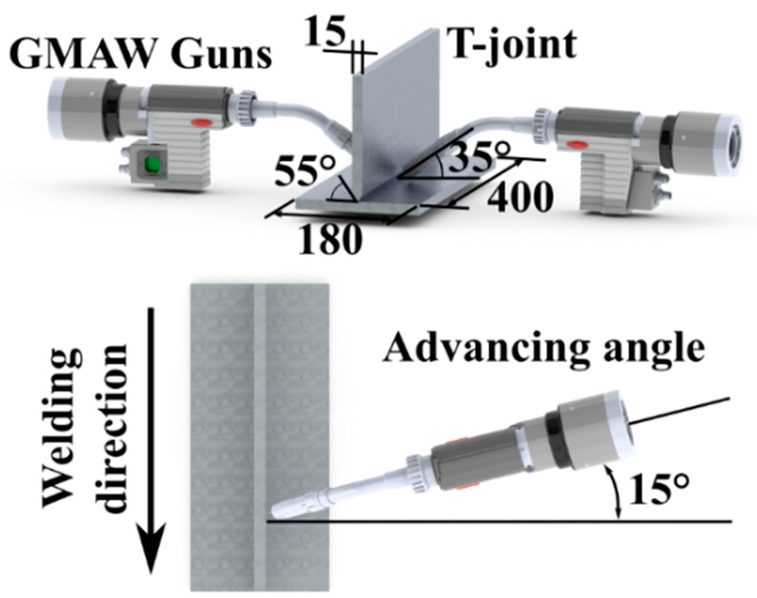
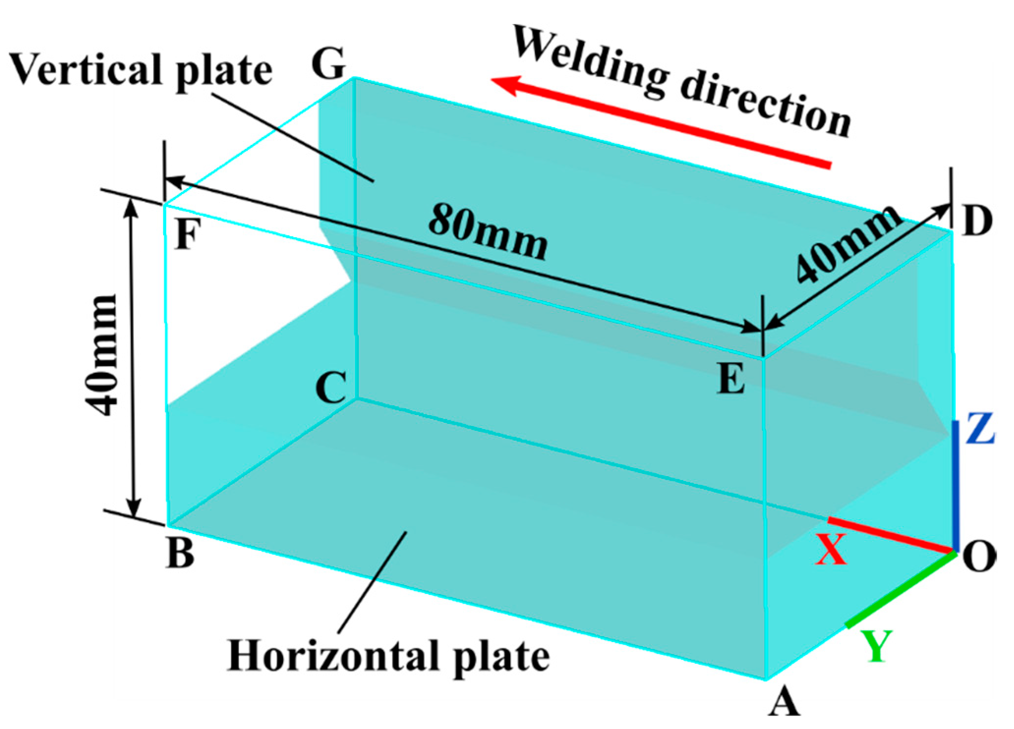
2.4. Computational Domain, Boundary Conditions

In this study, the 6082 aluminum alloy T-joint was chosen as the simulation target. As shown in Figure 3, the dimensions of the horizontal and vertical plate were 15 mm × 180 mm × 400 mm. The groove was beveled on both sides of the vertical plate with an angle of 55°, while a 2 mm root face was reserved. The axial direction formed an angle of 35° with the horizontal plate and 75° with the welding direction. For the symmetrical double-sided welding, only half of the T-joint was included in the computational domain to improve simulation efficiency, as shown in Figure 4. As the size of the computational domain was limited by computing capacity, the heat source stayed still during the simulation, while the T-joint moved backward. So, the simulated welding time could be very long, even if a small computational domain was used. A computational domain of 80 mm × 40 mm × 40 mm was chosen for simulation. The mesh size near the groove was set as 0.2 mm and transited to 0.6 mm near the boundary. For nonsymmetrical welding with a longitudinal torch distance, the full computational domain was used instead.

Two types of boundaries were included in our model. The first was the mesh block boundary, i.e., the boundary of the computational domain. In Figure 2, CBFG is the velocity inlet, while OAED is the velocity outlet. According to the relative motion mode mentioned above, the inlet velocity was set as equal to the welding speed. At the inlet surface, the cell was initialized selectively to keep the consistent geometrical shape of the T-joint groove. OCGD is the symmetric plane. On this plane, the gradients of state variables on the normal direction are equal to zero, and the normal velocity is zero:

$$\begin{array}{cc}\begin{array}{cc}\begin{array}{cc}\begin{array}{cc}\begin{array}{cc}\frac{\partial T}{\partial \overrightarrow{n}}=0,& \frac{\partial p}{\partial \overrightarrow{n}}=0,\end{array}& \frac{\partial u}{\partial \overrightarrow{n}}=0,\end{array}& \frac{\partial v}{\partial \overrightarrow{n}}=0,\end{array}& \frac{\partial w}{\partial \overrightarrow{n}}=0,\end{array}& {\overrightarrow{v}}_n=0\end{array}$$

(12)

where $\frac{\partial T}{\partial \overrightarrow{n}}=0$ and $\frac{\partial p}{\partial \overrightarrow{n}}=0$ means the normal temperature and pressure gradient are equal to zero, $\frac{\partial u}{\partial \overrightarrow{n}}=0$, $\frac{\partial v}{\partial \overrightarrow{n}}=0$ and $\frac{\partial w}{\partial \overrightarrow{n}}$ represent the zero normal velocity gradient, and $\overrightarrow{n}=0$ represents the zero normal velocity.

OABC is the wall boundary. On this plane, the normal velocity is zero, and heat exchange occurs between the fluid and the external environment:

$$\begin{array}{cc}{\overrightarrow{v}}_n=0,& k\frac{\partial T}{\partial \overrightarrow{n}}=-h_c\left(T-T_0\right)-\sigma \xi \left(T^4-T_0^4\right)\end{array}$$

(13)

where $\overrightarrow{n}=0$ represents the normal velocity, and the second equation describes the convection and radiation loss on the boundary.

ABFE and EFGD is the continuative boundary. This condition consists of zero normal derivatives at the boundary for all quantities, which is intended to represent a smooth continuation of the flow through the boundary.

Then, another boundary is the free surface of the molten pool. Arc pressure, surface tension pressure, and Marangoni stress were applied to this internal boundary. The arc pressure was assumed to follow Gaussian distribution, which is commonly recognized in the molten pool simulations [34]:

$$P_{arc}=-\frac{P_{max}}{2\pi {\sigma }_p}\exp \left(-\frac{r^2}{2{\sigma }_p^2}\right)$$

(14)

where P_arc is the arc pressure, P_max is the maximum pressure at the arc center, σ_p is the distribution parameter of arc pressure. During the calculation, the arc pressure was loaded in a similar way to the surface heat source. The cell on the free surface was tracked every timestep. The arc pressure exerted on every single cell was calculated and converted into the body force. Then, the body force was decomposed to x, y, and z axis, and added to the source of the momentum conservation equations.

The surface tension pressure on the normal direction of the free surface can be calculated by:

$$P_{st}=\gamma \kappa$$

(15)

where P_st is the surface tension pressure, γ is the surface tension, and κ is the curvature of the free surface.

Marangoni shear stress can be expressed as:

$${\tau }_{max}=\frac{\partial \gamma }{\partial T}\frac{\partial T}{\partial \overrightarrow{s}}$$

(16)

where τ_max is Marangoni shear stress and $\overrightarrow{s}$ is the unit tangent vector.

From which, the surface tension γ is calculated as follows:

$$\gamma ={\gamma }_0-\frac{d\gamma }{dT}\left(T-T_{ref}\right)$$

(17)

where γ₀ is the surface tension at the reference temperature and T_ref is the reference temperature.

The reliability and correctness of the above numerical model have been validated in our previously published research [44].

2.5. Simulated Welding Conditions

This study first chose a wire feed speed of 9 m/min to investigate the typical transient molten pool behavior. Then, conditions with wire feed speeds of 6 m/min, 7 m/min, and 8 m/min were supplemented to figure out the influences of wire feed speed on the fluid flow. Finally, nonsymmetrical double-sided welding with torch distances of 5 mm, 10 mm, 15 mm, and 20 mm were simulated to investigate the influences of torch distances. The welding parameters included in the eight different welding conditions are listed in

Table 1. Welding parameters included in different welding conditions.

Case No.	Wire Feed Speed (m/min)	Welding Speed (mm/s)	Droplet Transfer Frequency (Hz)	Wire Diameter (mm)	Torch Distance (mm)
1	9	5.6	220	1.2	0
2	7	5.6	132	1.2	0
3	8	5.6	178	1.2	0
4	10	5.6	214	1.2	0
5	9	5.6	220	1.2	5
6	9	5.6	220	1.2	10
7	9	5.6	220	1.2	15
8	9	5.6	220	1.2	20

.

3. Results and Discussion

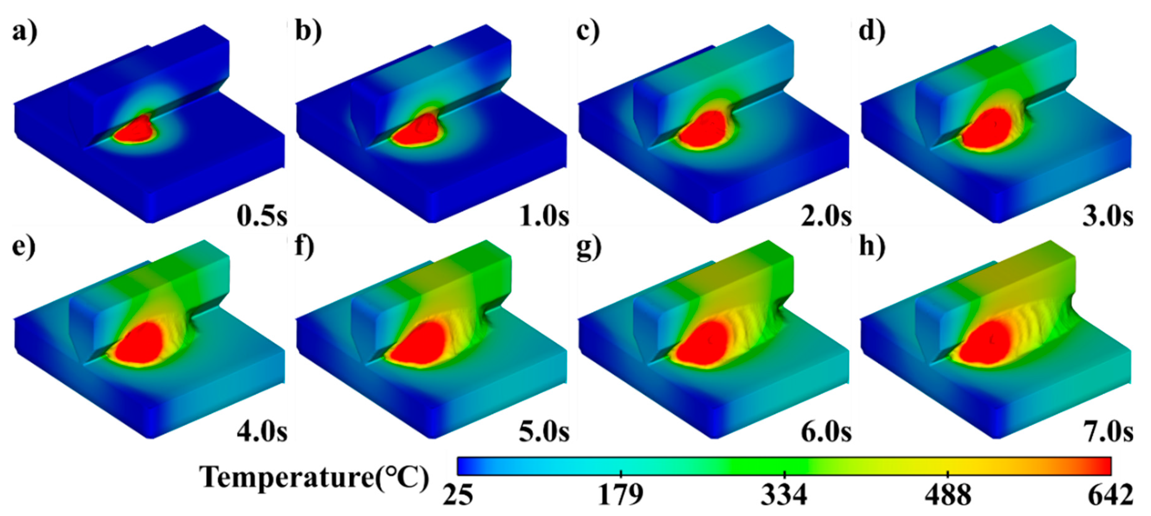
3.1. Basic Transient Molten Pool Behaviors

In the following section, the basic molten pool behaviors are discussed based on the results of Case 1. In Figure 5, the weld bead formation process is visualized using the transient temperature contours from the welding time of 0.5 s to 7.0 s. The red part represents the region whose temperature is higher than the liquidus temperature 642 ℃, i.e., the molten pool. The size of the molten pool increases with the welding time in the first 5 s and then stabilizes. Due to the impingement of droplets, the free surface at the molten pool center is concave. The fore part of the molten pool has a larger aspect ratio than the back part. This is the result of the 75° advancing angle (shown in Figure 3).

Then, the results at 7.0 s were chosen to illustrate the quasi-stable-state flow behaviors. The longitudinal section (Plane 1, the section parallel to the torch and cross the center of molten pool) and the cross-section (Plane 2, the section parallel to the YOZ plane and cross the center of the molten pool) at the same welding time are visualized in Figure 6 to help achieve a comprehensive understanding of the spatial flow characteristics. The black arrows in the figures are the velocity vectors. In Figure 6b, the velocity distribution shows that most of the molten pool surface has a velocity component towards the welding direction (the positive X direction). At the same time, Figure 6c demonstrates a frontward vortex on the longitudinal center plane. These two figures indicate the critical role of the advancing angle. With a non-vertical advancing angle, the droplet brings the momentum component to the welding direction, which drives the melt to flow frontward. Similar to the formation cause of finger-shaped penetration in a previously reported GMAW simulation [33], this also intensifies the convective heat transfer in the advancing direction, leading to a large aspect ratio in the front part of the molten pool. As shown by Figure 6d, the driving effect of droplet impinging is also significant on the cross-section. However, its influences are concentrated in the center of the molten pool. The velocity vector points to the centrifugal direction at the outside of the melting metal, which is annotated by white arrows in Figure 6d. This is the result of Marangoni stress. The vortex near the horizontal plate is larger than the other, demonstrating that gravity also has a small contribution. Then, the velocity magnitude on the two planes is visualized in Figure 6e,f. On the longitudinal section (Figure 6e), the maximum velocity lies on the top surface, while the vortex flow pattern leads to a relatively small velocity in the molten pool center. On the cross-section (Figure 6f), the maximum velocity lies on the falling position of the droplet. The results obtained agree quite well with previously reported ones. The leading driving effect of the droplet has also been illustrated in multiple independent simulations on the GMAW molten pool [23,28,30,43], even with altered welding positions [40]. In the pulsed GMAW of steel, the high flow speed region can move to the bottom of the molten pool with the droplet [30]. However, in this study, droplet influences on velocity magnitude were only concentrated near the free surface. This is the result of a much smaller droplet radius compared with [30]. The outward flow driven by Marangoni stress has also been verified via different simulation approaches [45,46]. It does play an essential role in autogenous welding. However, since the droplet has a significant axial transferring speed, the resistance to Marangoni stress is weak in the molten pool center, and the typical symmetry outward vortexes [44] are not witnessed. Although the welding process was not conducted in the flat welding position, the influences of gravity are relatively weak on flow behaviors. Similar phenomena were also reported in steels [31,40].

Figure 7 shows the temperature contours and velocity distributions at different welding times. The cross-section was also extracted at the droplet falling position shown in Figure 6a. The droplet transfer and Marangoni stress are the leading driving force throughout the whole welding process. The flow behaviors at different times are similar to those shown in Figure 6d.

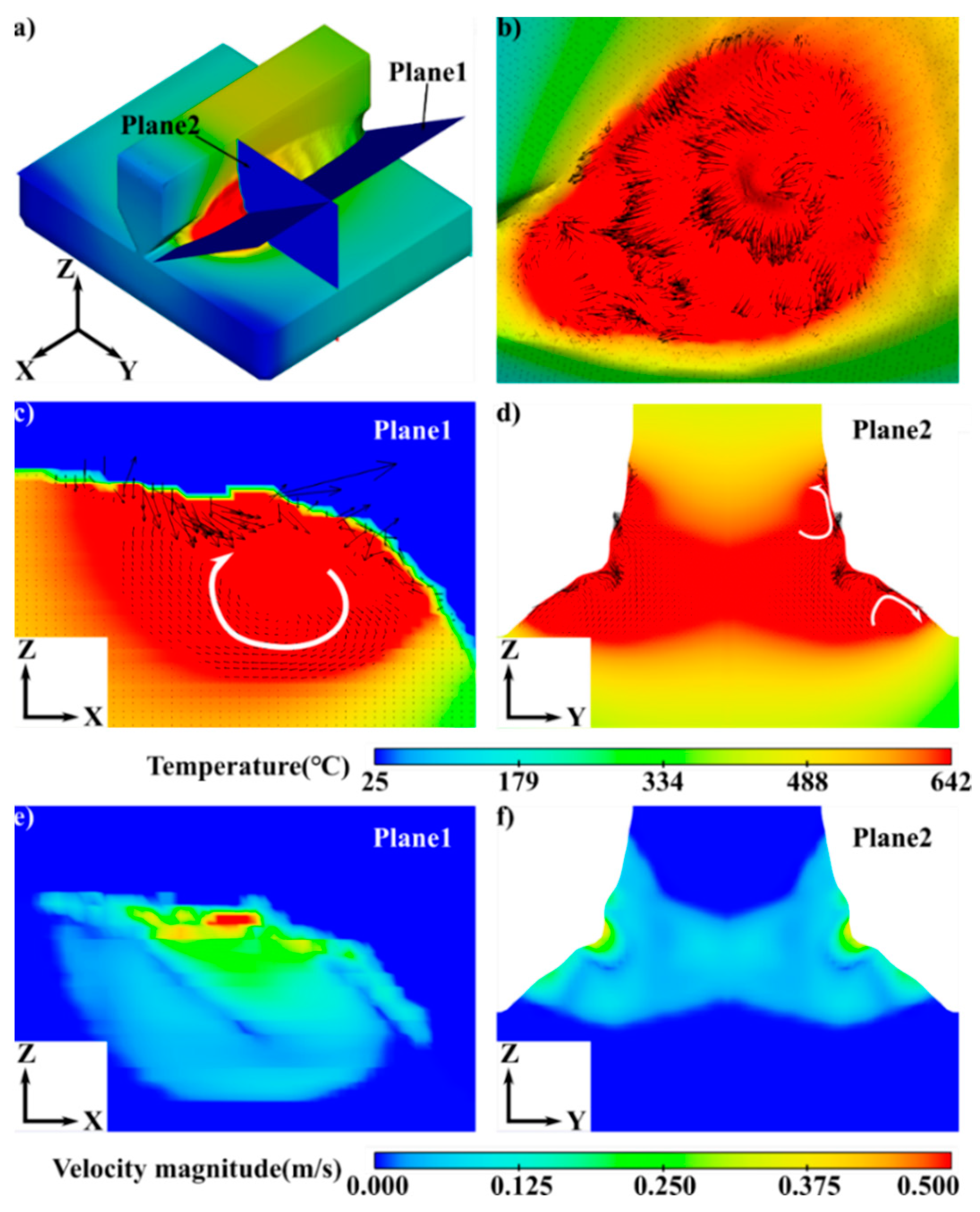
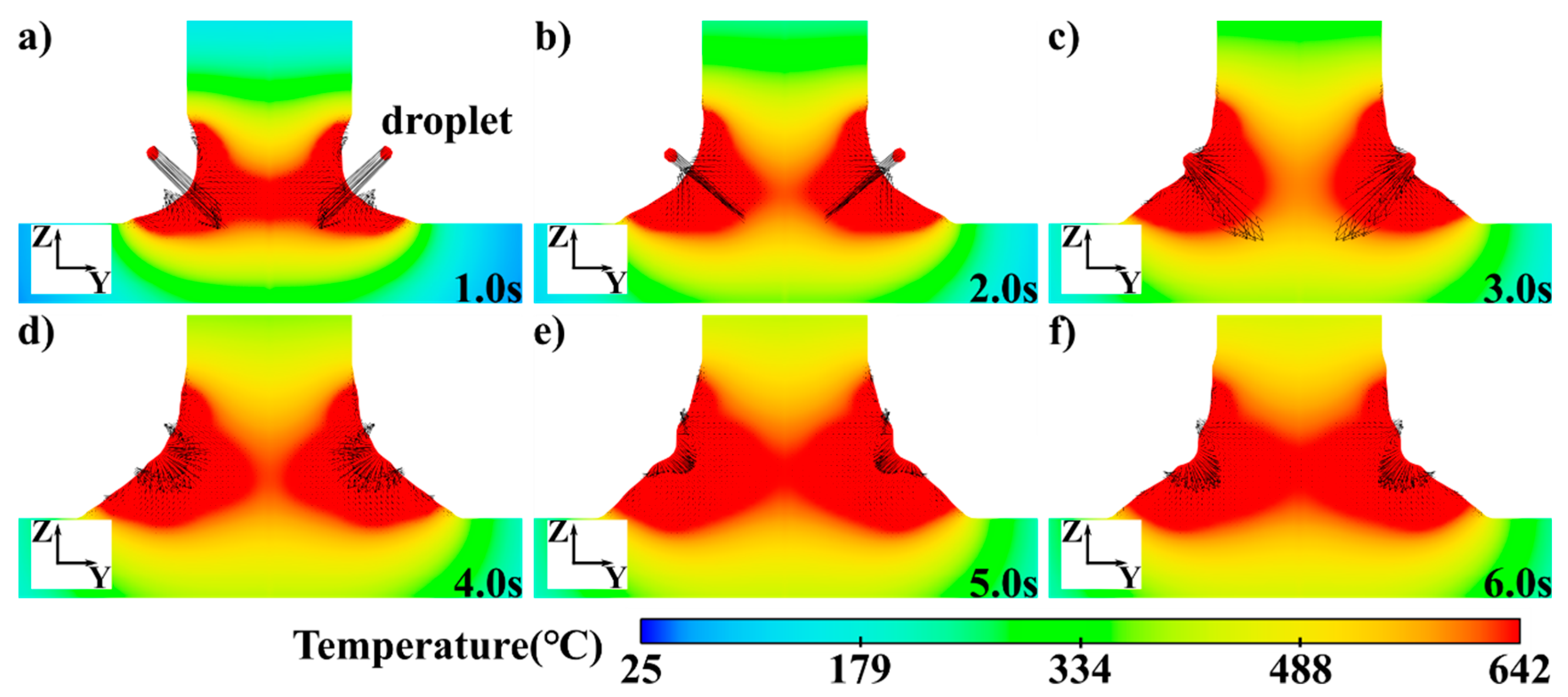
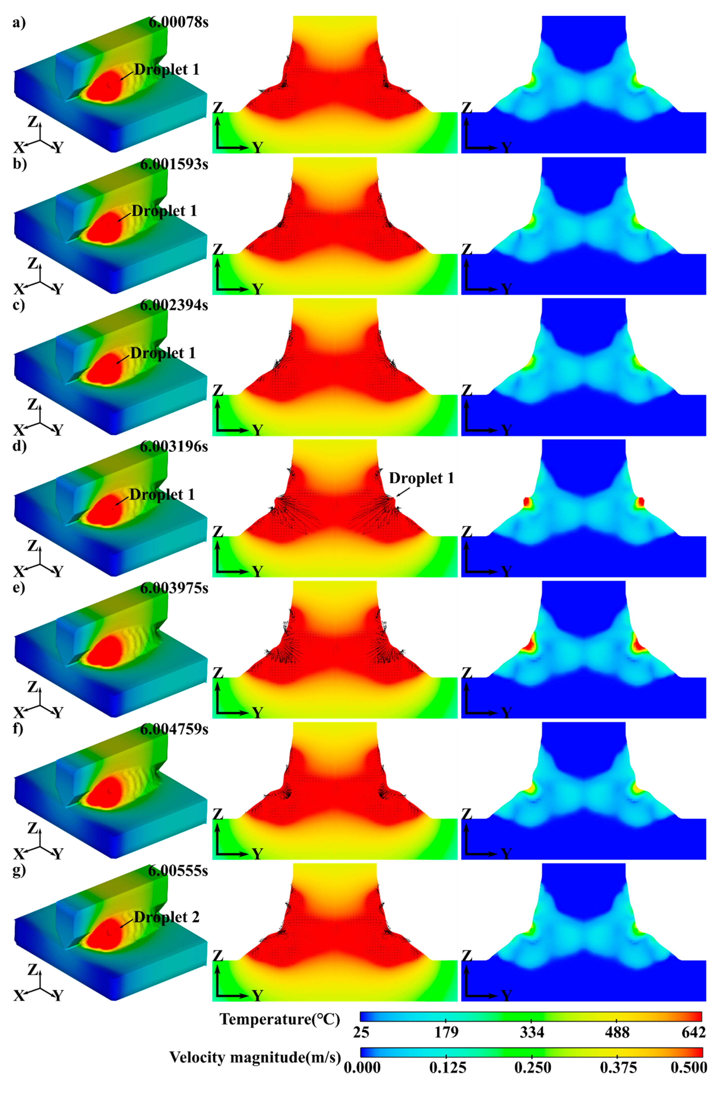
3.2. Fluid Flow during a Single Pulse Cycle

Then, we take a more in-depth look at the molten pool flow behaviors during a single pulse cycle. As shown by Figure 8, the first droplet investigated is generated at 6.00078 s. At this time, as shown by Figure 8a, the molten pool surface is still concave-shaped under the impingement of the last droplet. However, the Marangoni stress forces the fluid to close the pit. Thus, we witnessed a solid centripetal flow near the molten pool center, as shown by Figure 8b,c. Moreover, the concave surface is flattened quickly from 6.00078 s to 6.002394 s. At 6.003196 s, the droplet makes contact with the molten pool surface, bringing intense axial momentum, as shown by the vectors and the red region in Figure 8d. Furthermore, the molten pool surface becomes concave again. Similar effects of Marangoni stress after droplet transfer were also reported in [30]. It plays an important role in maintaining the uniform weld bead appearance.

After the impingement of the droplet, the axial flow in the molten pool center is hindered quickly by the pressure resistance inside the melted metal. Additionally, at the same time, Marangoni stress acts again, generating centripetal flow to flatten the molten pool surface. At 6.00555 s, as shown by Figure 8g, another droplet is generated, a new pulse cycle starts, and the above process repeats again. The molten pool center has the largest flow velocity during the whole cycle, and the maximum velocity significantly increases when the droplet interacts with the molten pool. However, comparing the temperature contours in Figure 8a to Figure 8g, although the weld current experiences a drastic change during a single pulse cycle, the temperature distribution remains constant. This is caused by the intrinsic nature of welding heat transfer. During the pulsed GMAW with a high frequency, arc heat transfer to the molten pool bottom relies on convection. In such a short time current pulse, the influences of the heat input variation on the molten pool surface are much weaker than the energy input by droplet transfer. Thus, the temperature contours experience minimal changes; similar results were obtained by [30]. It should be noted that when the pulse frequency is relatively low, the circumstance will be different. As presented by [32], the molten pool size evolution with a current pulse less than 10 Hz was significant. This is because the peak and the base current time are relatively longer, the influences of arc energy change can be introduced to the whole molten pool with the effective help of convection.

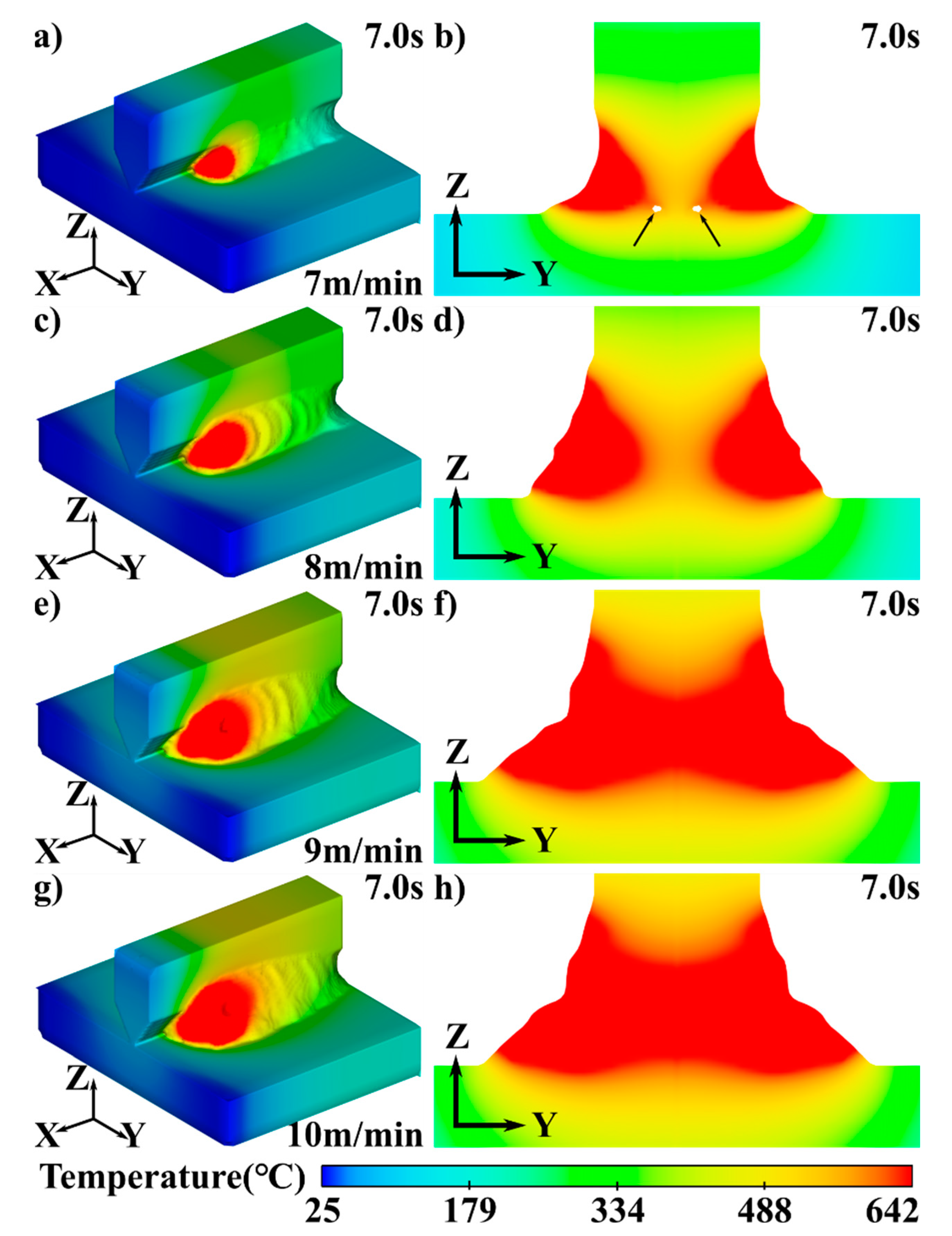
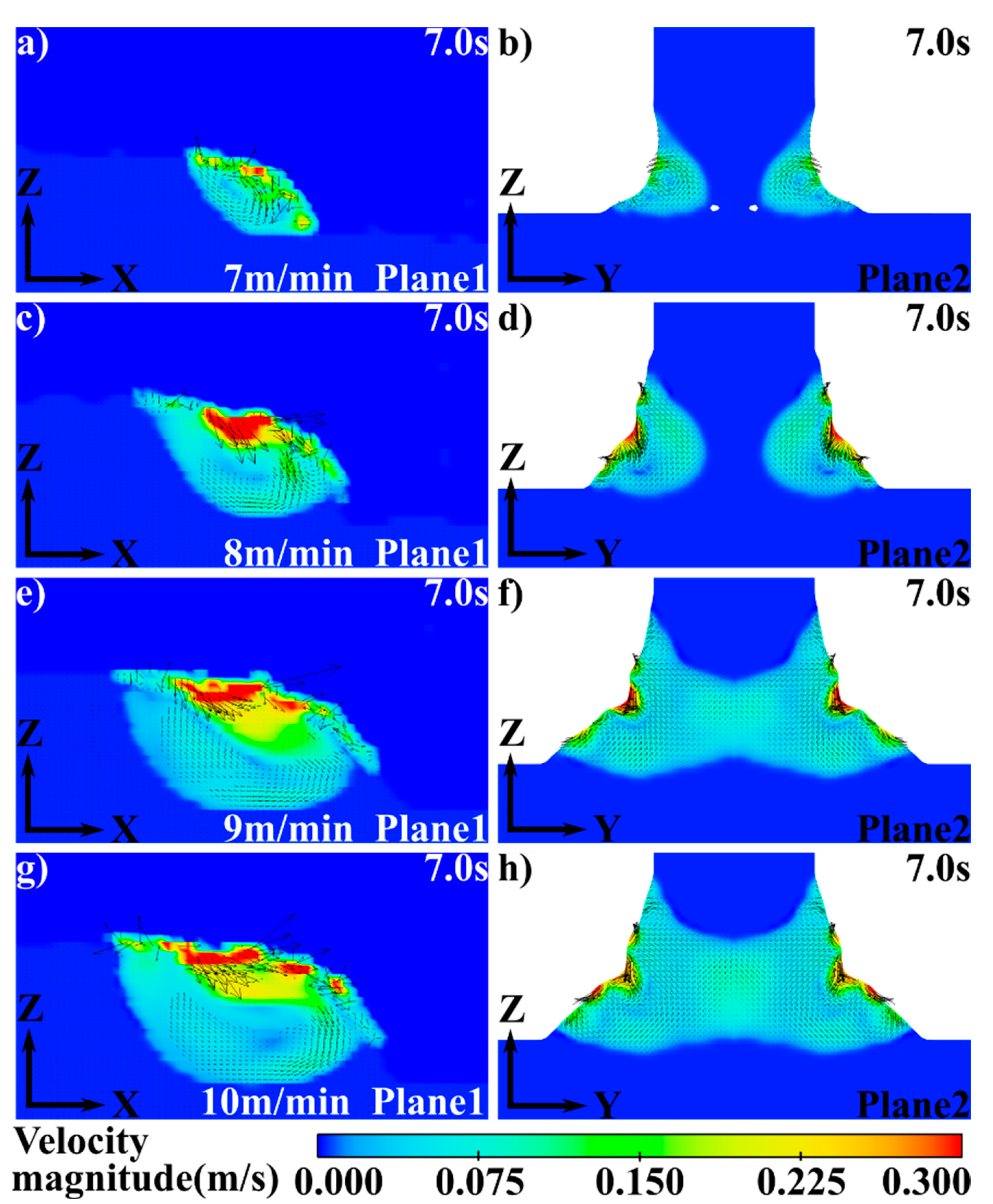
3.3. Influences of the Wire Feed Speed

The calculation results of Cases 1, 2, 3, and 4 are compared to investigate the influences of wire feed speed. At first, the temperature distributions on the model surface and molten pool cross sections are displayed in Figure 9. The cross sections are also extracted at the location shown by 6a. As the wire feed speed increases, the volume of the molten pool also increases significantly due to more extensive heat input. When a wire feed speed of 7 m/min is applied, as shown by Figure 9b, the energy input is not large enough for a good spreading of melted metal. A lack of fusion is found near the root of the weld bead. As the feed rates rise to 8 m/min, as shown by Figure 9d, the root fusion is improved. However, the penetration is still not enough for a solid joint between horizontal and vertical plates. When the wire feed rate is larger than 9 m/min (Figure 9f,h), full penetration is achieved.

Then, in Figure 10, the velocity magnitude contours and velocity vectors are visualized on the molten pool’s longitudinal section and cross-section. The extracting positions of clip planes are shown in Figure 6a. It can be seen that the wire feed speed does not change the basic flow feature of the frontward vortex on the longitudinal section. The droplet impingement is still the critical driving force. Moreover, the highest velocity magnitude appears near the droplet falling position. In general, the upper half of the vortex has a larger velocity magnitude than the lower part. Additionally, the area of the vortex increases with a larger molten pool size when applying a higher wire feed speed. On the cross-section, the interplay between droplet impingement and Marangoni stress is also witnessed. Although higher wire feed speed leads to a larger droplet transfer speed, its influences on the velocity magnitude mainly act near the molten pool surface. On the longitudinal section, a larger high-velocity area is witnessed using larger wire feed speed. However, the velocity magnitude inside the molten pool shows weak correlations with the wire feed speed.

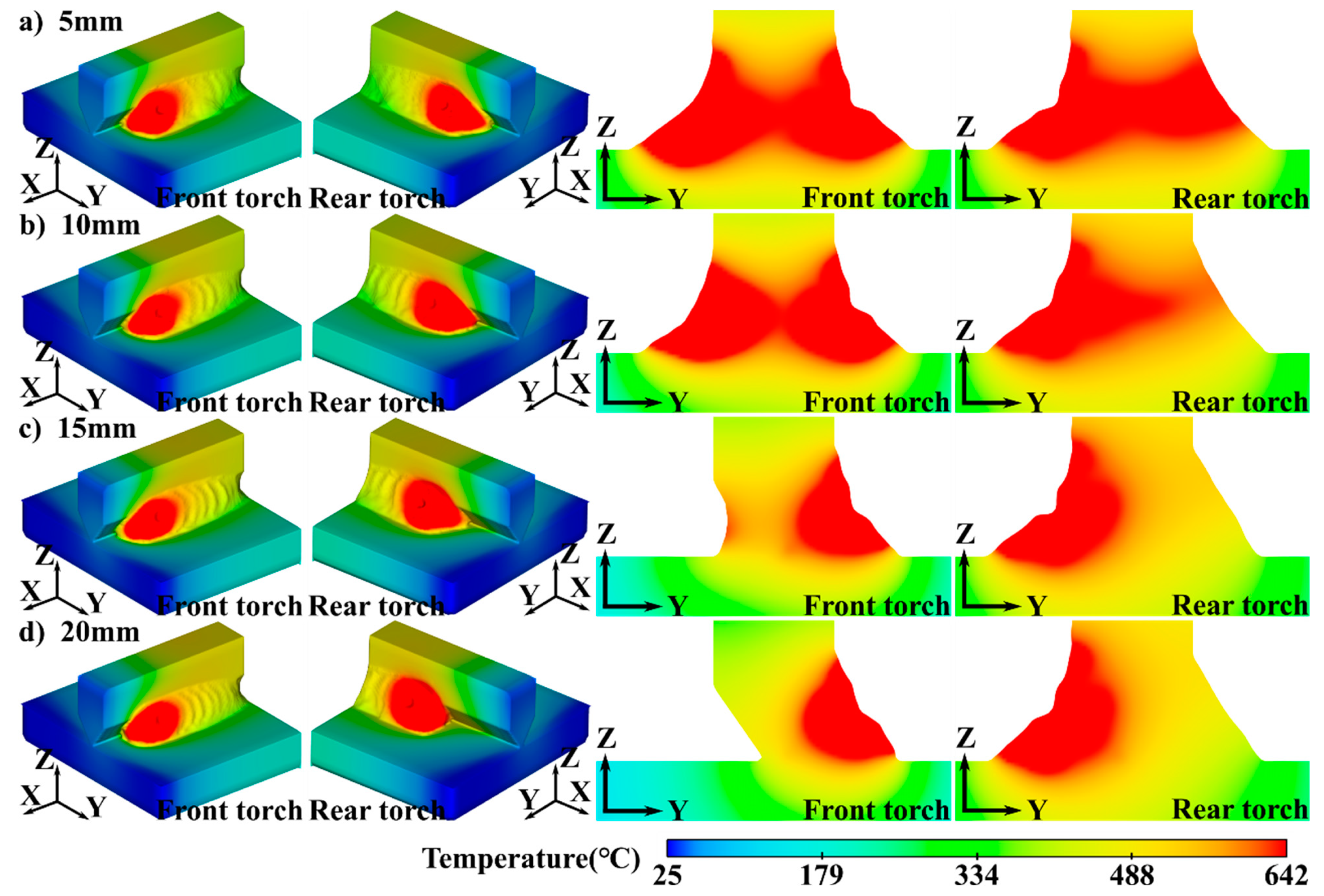
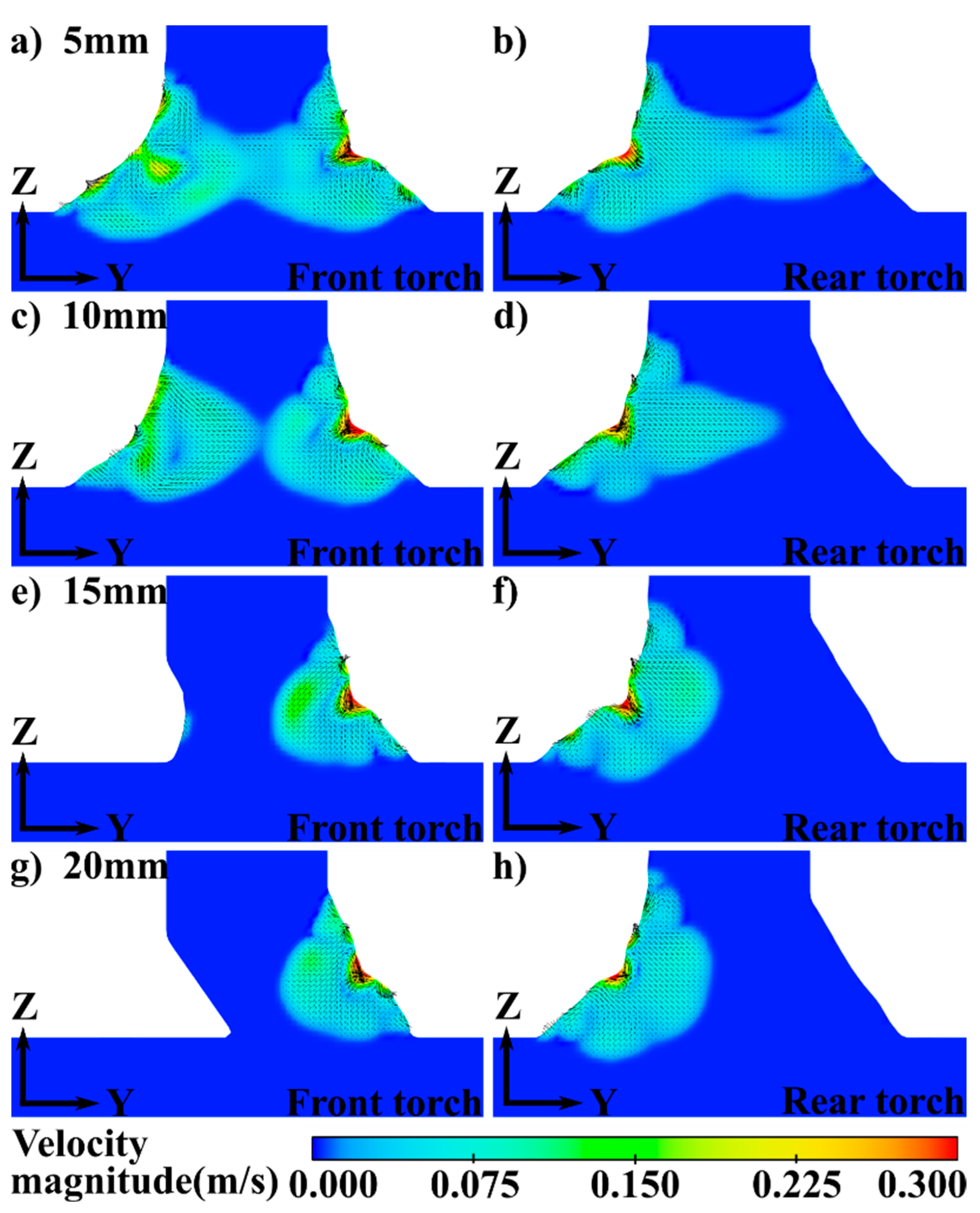
3.4. Influences of the Torch Distance

Finally, the influences of torch distances are discussed based on the calculation results of Case 5, 6, 7, and 8. Figure 11 shows the temperature contours at a welding time of 7.0 s on the model surfaces and cross-sections. Since the two weld torches are now placed at a non-symmetry position, the contours on the front and rear torch side are displayed, respectively, in the first and second column of Figure 11, and the contours on molten pool cross-sections through the center of the front and rear droplet transfer position are displayed separately in the third and fourth column of the assembly figure. As shown by the contours on the model surfaces, as the torch distance increases, the width of the front molten pool decreases, and the length rises. The reduced width results from decreased heat input on the other side, while the increased length attributes to the retarded cooling effects of the rear arc. For the rear molten pool, as the torch distance diminishes, the molten pool size decreases slightly.

Then, we take a closer look into the cross-section (the third and fourth column of Figure 11). It can be seen that, with a closer torch distance, the two molten pool has stronger interactions, and the penetration of both sides decreases. Since the front arc always has a preheating effect for the rear molten pool, the rear molten pool has a significantly larger amount of penetration. Then, the velocity distributions at 7.0 s on two cross-sections are shown in Figure 12. Despite the different molten pool sizes, the fluid flow characteristics are the same as the double-sided symmetry welding. On the pool surface, the liquid metal flows inward under the impinging of the droplets, and Marangoni stress drives the fluid to form two outward vortexes near the boundary. This indicates that compared with the two critical driving factors of fluid flow in the molten pools, the interactions between the molten pools on different sides have very limited effects on the flow behaviors of liquid metal.

4. Conclusions

In this work, a 3D numerical model was established to simulate the fluid flow during double-sided pulsed GMAW of aluminum T-joints. The model assumed that the fluid flow in the weld pool was laminar and incompressible, effects of the arc could be simplified as thermal and mechanical interactions, influences of metal vapor could be ignored, and the heterogeneity of materials could be ignored. Mass, momentum, energy, and VOF conservation equations were adopted as controlling equations. A transient adaptive heat source was applied to model the heat input on the free surface of the weld pool. With the numerical model, molten pool behaviors under different wire feed speeds and torch distances were visualized and investigated. The main results are summarized as follows:

1. The droplet impinging effect and Marangoni stress are the leading driving forces during the double-sided pulsed GMAW of T-joints. Under the counterbalance of the two forces, the melts form a frontward vortex on the longitudinal section. On the cross-section, the fluid near the center flows downward to the root, while the metal liquid the outside flows centrifugally.

2. During a single pulse cycle, there is an interplay between the influences of Marangoni stress and the droplet impingement. When the droplet transfers to the molten pool, strong axial momentum leads to an axial inward flow in the molten pool center, and the free surface becomes concave-shaped. Then, Marangoni stress acts to flatten the free surface as the pressure resistance weakens the inward flow. The temperature distribution is insensitive to the current variation in such a short time.

3. When using a higher wire feed speed, the volume of the molten pool increases, and root fusion is improved. With a wire feed speed larger than 9 m/min, full penetration can be achieved. Wire feed speed shows no significant effects on the basic fluid flow characteristics in the molten pool, and its influences on the velocity magnitude only act near the top surface.

4. As the torch distance increases, the width of the front molten pool decreases while the length increases, and the rear molten pool size decreases lightly. The interaction between two molten pools is compromised, and penetration differences between two molten pools appear. However, the torch distance has minimal effects on the fluid flow behaviors.

It should be noted that the microstructures and mechanical properties of the welded joint are of the same importance as the intrinsic physical phenomenon during the welding process. Readers are advised to refer to the upcoming article on the quality evaluation of the T-joints to relate the molten pool behaviors with the final quality of the welded T-joints.

References

1. Prajapati, P.; Badheka, V.J.; Mehta, K. An Outlook on Comparison of Hybrid Welds of Different Root Pass and Filler Pass of FCAW and GMAW with Classical Welds of Similar Root Pass and Filler Pass. Sādhanā 2018, 43, 75. [Google Scholar] [CrossRef] [Green Version]
2. Prajapati, P.; Badheka, V.J.; Mehta, K.P. Hybridization of Filler Wire in Multi-Pass Gas Metal Arc Welding of SA516 Gr70 Carbon Steel. Mater. Manuf. Process. 2018, 33, 315–322. [Google Scholar] [CrossRef]
3. Giętka, T.; Ciechacki, K.; Kik, T. Numerical Simulation of Duplex Steel Multipass Welding. Arch. Metall. Mater. 2016, 61, 1975–1984. [Google Scholar] [CrossRef] [Green Version]
4. Kik, T.; Górka, J.; Kotarska, A.; Poloczek, T. Numerical Verification of Tests on the Influence of the Imposed Thermal Cycles on the Structure and Properties of the S700MC Heat-Affected Zone. Metals 2020, 10, 974. [Google Scholar] [CrossRef]
5. Kik, T.; Moravec, J.; Novakova, I. Numerical Simulations of X22CrMoV12-1 Steel Multilayer Welding. Arch. Metall. Mater. 2019, 64, 1441–1448. [Google Scholar] [CrossRef]
6. Kik, T.; Moravec, J.; Novakova, I. New Method of Processing Heat Treatment Experiments with Numerical Simulation Support. IOP Conf. Ser. Mater. Sci. Eng. 2017, 227, 012069. [Google Scholar] [CrossRef] [Green Version]
7. Chang, K.-H.; Lee, C.-H. Finite Element Analysis of the Residual Stresses in T-Joint Fillet Welds Made of Similar and Dissimilar Steels. Int. J. Adv. Manuf. Technol. 2009, 41, 250–258. [Google Scholar] [CrossRef]
8. Luca, A.D.; Greco, A.; Mazza, P.; Caputo, F. Numerical Investigation on the Residual Stresses in Welded T-Joints Made of Dissimilar Materials. Procedia Struct. Integr. 2019, 24, 800–809. [Google Scholar] [CrossRef]
9. Zhang, Q.; Ma, Y.; Cui, C.; Chai, X.; Han, S. Experimental Investigation and Numerical Simulation on Welding Residual Stress of Innovative Double-Side Welded Rib-to-Deck Joints of Orthotropic Steel Decks. J. Constr. Steel Res. 2021, 179, 106544. [Google Scholar] [CrossRef]
10. Khoshroyan, A.; Darvazi, A.R. Effects of Welding Parameters and Welding Sequence on Residual Stress and Distortion in Al6061-T6 Aluminum Alloy for T-Shaped Welded Joint. Trans. Nonferrous Met. Soc. China 2020, 30, 76–89. [Google Scholar] [CrossRef]
11. Zhang, C.; Li, S.; Hu, L.; Deng, D. Effects of Pass Arrangement on Angular Distortion, Residual Stresses and Lamellar Tearing Tendency in Thick-Plate T-Joints of Low Alloy Steel. J. Mater. Process. Technol. 2019, 274, 116293. [Google Scholar] [CrossRef]
12. Zhang, C.; Li, S.; Sun, J.; Wang, Y.; Deng, D. Controlling Angular Distortion in High Strength Low Alloy Steel Thick-Plate T-Joints. J. Mater. Process. Technol. 2019, 267, 257–267. [Google Scholar] [CrossRef]
13. Chu, Q.; Kong, X.; Tan, W. Introducing Compressive Residual Stresses into a Stainless-Steel T-Pipe Joint by an Overlay Weld. Metals 2021, 11, 1109. [Google Scholar] [CrossRef]
14. Perić, M.; Tonković, Z.; Rodić, A.; Surjak, M.; Garašić, I.; Boras, I.; Švaić, S. Numerical Analysis and Experimental Investigation of Welding Residual Stresses and Distortions in a T-Joint Fillet Weld. Mater. Des. 2014, 53, 1052–1063. [Google Scholar] [CrossRef]
15. Rong, Y.; Zhang, G.; Huang, Y. Study on Deformation and Residual Stress of Laser Welding 316L T-Joint Using 3D/Shell Finite Element Analysis and Experiment Verification. Int. J. Adv. Manuf. Technol. 2017, 89, 2077–2085. [Google Scholar] [CrossRef]
16. Liang, W.; Hu, X.; Zheng, Y.; Deng, D. Determining Inherent Deformations of HSLA Steel T-Joint under Structural Constraint by Means of Thermal Elastic Plastic FEM. Thin-Walled Struct. 2020, 147, 106568. [Google Scholar] [CrossRef]
17. Lan, X.; Chan, T.-M.; Young, B. Structural Behaviour and Design of High Strength Steel CHS T-Joints. Thin-Walled Struct. 2021, 159, 107215. [Google Scholar] [CrossRef]
18. Lan, X.; Chan, T.-M.; Young, B. Testing, Finite Element Analysis and Design of High Strength Steel RHS T-Joints. Eng. Struct. 2021, 227, 111184. [Google Scholar] [CrossRef]
19. Luo, P.; Asada, H.; Tanaka, T. Limit Analysis for Partial-Joint-Penetration Weld T-Joints with Arbitrary Loading Angles. Eng. Struct. 2020, 213, 110459. [Google Scholar] [CrossRef]
20. Matti, F.N.; Mashiri, F.R. Experimental and Numerical Studies on SCFs of SHS T-Joints Subjected to Static out-of-Plane Bending. Thin-Walled Struct. 2020, 146, 106453. [Google Scholar] [CrossRef]
21. Gadallah, R.; Tsutsumi, S.; Tanaka, S.; Osawa, N. Accurate Evaluation of Fracture Parameters for a Surface-Cracked Tubular T-Joint Taking Welding Residual Stress into Account. Mar. Struct. 2020, 71, 102733. [Google Scholar] [CrossRef]
22. Kou, S.; Sun, D.K. Fluid Flow and Weld Penetration in Stationary Arc Welds. Metall. Trans. A 1985, 16, 11. [Google Scholar] [CrossRef]
23. Cho, D.-W.; Na, S.-J.; Cho, M.-H.; Lee, J.-S. Simulations of Weld Pool Dynamics in V-Groove GTA and GMA Welding. Weld World 2013, 57, 223–233. [Google Scholar] [CrossRef]
24. Cho, D.-W.; Na, S.-J. Molten Pool Behaviors for Second Pass V-Groove GMAW. Int. J. Heat Mass Transf. 2015, 88, 945–956. [Google Scholar] [CrossRef]
25. Bahrami, A.; Helenbrook, B.T.; Valentine, D.T.; Aidun, D.K. Fluid Flow and Mixing in Linear GTA Welding of Dis-similar Ferrous Alloys. Int. J. Heat Mass Transf. 2016, 93, 729–741. [Google Scholar] [CrossRef]
26. Jeong, H.; Park, K.; Kim, Y.; Kim, D.-Y.; Kang, M.-J.; Cho, J. Numerical Analysis of Weld Pool for Galvanized Steel with Lap Joint in GTAW. J. Mech. Sci. Technol. 2017, 31, 2975–2983. [Google Scholar] [CrossRef]
27. Hao, H.; Gao, J.; Huang, H. Numerical Simulation for Dynamic Behavior of Molten Pool in Tungsten Inert Gas Welding with Reserved Gap. J. Manuf. Process. 2020, 58, 11–18. [Google Scholar] [CrossRef]
28. Cho, D.-W.; Park, J.-H.; Moon, H.-S. A Study on Molten Pool Behavior in the One Pulse One Drop GMAW Process Using Computational Fluid Dynamics. Int. J. Heat Mass Transf. 2019, 139, 848–859. [Google Scholar] [CrossRef]
29. Wang, D.; Lu, H. Numerical Analysis of Internal Flow of Molten Pool in Pulsed Gas Tungsten Arc Welding Using a Fully Coupled Model with Free Surface. Int. J. Heat Mass Transf. 2021, 165, 120572. [Google Scholar] [CrossRef]
30. Ikram, A.; Chung, H. Numerical Simulation of Arc, Metal Transfer and Its Impingement on Weld Pool in Variable Polarity Gas Metal Arc Welding. J. Manuf. Process. 2021, 64, 1529–1543. [Google Scholar] [CrossRef]
31. Traidia, A.; Roger, F.; Schroeder, J.; Guyot, E.; Marlaud, T. On the Effects of Gravity and Sulfur Content on the Weld Shape in Horizontal Narrow Gap GTAW of Stainless Steels. J. Mater. Process. Technol. 2013, 213, 1128–1138. [Google Scholar] [CrossRef]
32. Liu, J.W.; Rao, Z.H.; Liao, S.M.; Tsai, H.L. Numerical Investigation of Weld Pool Behaviors and Ripple Formation for a Moving GTA Welding under Pulsed Currents. Int. J. Heat Mass Transf. 2015, 91, 990–1000. [Google Scholar] [CrossRef]
33. Cheon, J.; Kiran, D.V.; Na, S.-J. CFD Based Visualization of the Finger Shaped Evolution in the Gas Metal Arc Welding Process. Int. J. Heat Mass Transf. 2016, 97, 1–14. [Google Scholar] [CrossRef]
34. Meng, X.; Qin, G.; Zou, Z. Investigation of Humping Defect in High Speed Gas Tungsten Arc Welding by Numerical Modelling. Mater. Des. 2016, 94, 69–78. [Google Scholar] [CrossRef]
35. Pan, J.; Hu, S.; Yang, L.; Wang, D. Investigation of Molten Pool Behavior and Weld Bead Formation in VP-GTAW by Numerical Modelling. Mater. Des. 2016, 111, 600–607. [Google Scholar] [CrossRef]
36. Hamed Zargari, H.; Ito, K.; Kumar, M.; Sharma, A. Visualizing the Vibration Effect on the Tandem-Pulsed Gas Metal Arc Welding in the Presence of Surface Tension Active Elements. Int. J. Heat Mass Transf. 2020, 161, 120310. [Google Scholar] [CrossRef]
37. Qin, G.; Feng, C.; Ma, H. Suppression Mechanism of Weld Appearance Defects in Tandem TIG Welding by Numerical Modeling. J. Mater. Res. Technol. 2021, 14, 160–173. [Google Scholar] [CrossRef]
38. Qiao, J.; Wu, C.; Li, Y. Numerical Analysis of Keyhole and Weld Pool Behaviors in Ultrasonic-Assisted Plasma Arc Welding Process. Materials 2021, 14, 703. [Google Scholar] [CrossRef] [PubMed]
39. Jian, X.; Wu, H. Influence of the Longitudinal Magnetic Field on the Formation of the Bead in Narrow Gap Gas Tungsten Arc Welding. Metals 2020, 10, 1351. [Google Scholar] [CrossRef]
40. Hu, Z.; Hua, L.; Qin, X.; Ni, M.; Ji, F.; Wu, M. Molten Pool Behaviors and Forming Appearance of Robotic GMAW on Complex Surface with Various Welding Positions. J. Manuf. Process. 2021, 64, 1359–1376. [Google Scholar] [CrossRef]
41. Xu, W.H.; Dong, C.L.; Zhang, Y.P.; Yi, Y.Y. Characteristics and Mechanisms of Weld Formation during Oscillating Arc Narrow Gap Vertical up GMA Welding. Weld World 2017, 61, 241–248. [Google Scholar] [CrossRef]
42. Lang, R.; Han, Y.; Bai, X.; Hong, H. Prediction of the Weld Pool Stability by Material Flow Behavior of the Perforated Weld Pool. Materials 2020, 13, 303. [Google Scholar] [CrossRef] [PubMed] [Green Version]
43. Zhu, C.; Cheon, J.; Tang, X.; Na, S.-J.; Lu, F.; Cui, H. Effect of Swing Arc on Molten Pool Behaviors in Narrow-Gap GMAW of 5083 Al-Alloy. J. Mater. Process. Technol. 2018, 259, 243–258. [Google Scholar] [CrossRef]
44. Cai, X.; Dong, B.; Lin, S.; Murphy, A.B.; Fan, C.; Yang, C. Heat Source Characteristics of Ternary-Gas-Shielded Tandem Narrow-Gap GMAW. Materials 2019, 12, 1397. [Google Scholar] [CrossRef] [PubMed] [Green Version]
45. Saso, S.; Mouri, M.; Tanaka, M.; Koshizuka, S. Numerical Analysis of Two-Dimensional Welding Process Using Particle Method. Weld World 2016, 60, 127–136. [Google Scholar] [CrossRef] [Green Version]
46. Cho, W.-I.; Na, S.-J.; Kim, C.-H. Influence of Driving Forces on Weld Pool Dynamics in GTA and Laser Welding. Weld World 2013, 57, 257–264. [Google Scholar] [CrossRef]
Figure 1. The adaptive heat source.
Metals 11 01594 g001
Figure 2. Time-dependent voltage and current table.
Metals 11 01594 g002
Figure 3. Schematic diagram of T-joint double-sided GMA welding.
Metals 11 01594 g003
Figure 4. Computational domain.
Metals 11 01594 g004
Figure 5. Weld bead formation process: weld bead appearance visualized by temperature contours at (a) 0.5 s, (b) 1.0 s, (c) 2.0 s, (d) 3.0 s, (e) 4.0 s, (f) 5.0 s, (g) 6.0 s, and (h) 7.0 s.
Metals 11 01594 g005
Figure 6. Molten pool flow characteristics: (a) locations of clip planes; velocity vectors on the (b) top surface, (c) longitudinal section, and (d) cross-section of the molten pool; velocity magnitude distribution on the (e) longitudinal section, and (f) cross-section of the weld bead.
Metals 11 01594 g006
Figure 7. Transient evolution of velocity vectors on the cross section of molten pool: (a) 1.0 s; (b) 2.0 s; (c) 3.0 s; (d) 4.0 s; (e) 5.0 s; (f) 6.0 s.
Metals 11 01594 g007
Figure 8. Molten pool behaviors during a single pulse cycle: weld bead appearance (the first column), temperature contours with velocity vectors on the cross sections (the second column), and velocity magnitude distribution on the cross sections (the third column) at (a) 6.0078 s, (b) 6.001593 s, (c) 6.002394 s, (d) 6.003196 s, (e) 6.003975 s, (f) 6.004759 s, and (g) 6.00555 s.
Metals 11 01594 g008
Figure 9. Temperature distributions on the model surface: wire feed speeds of (a) 7 m/min, (c) 8 m/min, (e) 9 m/min, (g) 10 m/min; temperature distributions on the cross sections: wire feed speeds of (b) 7 m/min, (d) 8 m/min, (f) 9 m/min, and (h) 10 m/min.
Metals 11 01594 g009
Figure 10. Velocity distributions on the longitudinal sections: wire feed speeds of (a) 7 m/min, (c) 8 m/min, (e) 9 m/min, and (g) 10 m/min; velocity distributions on the cross sections: wire feed speeds of (b) 7 m/min, (d) 8 m/min, (f) 9 m/min, (h) 10 m/min.
Metals 11 01594 g010
Figure 11. Temperature distribution on the model surface (the first and second column) and cross-section (the third and fourth column) at the welding time of 7.0 s: torch distances of (a) 5 mm, (b) 10 mm, (c) 15 mm, and (d) 20 mm.
Metals 11 01594 g011
Figure 12. Velocity distribution and velocity vectors on the cross-sections: (a) 5 mm front torch, (b) 5 mm rear torch, (c) 10 mm front torch, (d) 10 mm rear torch, (e) 15 mm front torch, (f) 15 mm-rear torch, (g) 20 mm front torch, and (h) 20 mm rear torch.
Metals 11 01594 g012