Neuro-Fuzzy System for Compensating Slow Disturbances in Adaptive Mold Level Control

Abstract

Good slow disturbances attenuation in a mold level control with stopper rod is very important for avoiding several product defects and keeping down casting interruptions. The aim of this work is to improve the accuracy of the diagnosis and compensation of an adaptive mold level control method for slow disturbances related to changes of stopper rod. The advantages offered by the architecture, called Adaptive-Network-based Fuzzy Inference System, were used for training a previous model. This allowed learning based on the process data from a steel cast case study, representing all intensity levels of valve erosion and clogging. The developed model has high accuracy in its functional relationship between two compact input variables and the compensation coefficient of the valve gain variations. The future implementation of this proposal will consider a combined training of the model, which would be very convenient for maintaining good accuracy in the Fuzzy Inference System using new data from the process.

1. Introduction

Continuous casting is a process where molten metal is solidified into a semi-finished billet, bloom, or slab for subsequent rolling in finishing mills; it is the most frequently used process for steel casting. It allows lower-cost production of metal sections with better quality, due to the inherently lower costs of continuous, standardized production of the product, as well as providing increased control over the process through automation [1]. Complex control tasks such as the mold level control (MLC) are very important for avoiding several product defects and keeping down casting interruptions [2]. The mold level fluctuations may produce many quality problems [3]. Level fluctuations can be caused by different types of disturbance: periodic, slow and sudden [4,5]. Among these, compensation for MLC slow disturbances such as valve erosion and valve clogging are insufficiently resolved problems.

From the metallurgical point of view, many investigations have studied the steel defects caused by mold level fluctuations [3,4,6,7,8,9,10,11,12,13]. From the control point of view, the proposed solutions have been designed to compensate for the typical characteristics of the disturbances that cause mold level fluctuations in each case study. In practice, to eliminate the defects caused by periodic, slow and sudden disturbances in an MLC, efficient integration of various control techniques is required. Particularly, slow disturbances, related to valve erosion and clogging in an MLC with stopper rod (SR), have been considered by some authors [2,4,14,15,16].

Robin De Keyser indicated that the process characteristics for a MLC with SR, especially plant gain, can be expected to strongly vary during operation and a good control design should take this into account. The author states that valve erosion or valve clogging leads to changes in effective gain. When testing the robustness of the designed controllers for one steel continuous casting machine, a total variation of as much as 400% in plant gain was applied [14]. In [15], according to the authors’ estimations, the values of plant gain usually vary by up to 300%, and they propose a robust control approach.

A figure with SR with typical characteristics, including the two types of disturbance, valve clogging and valve erosion, was presented by Smutný et al. [16]. They also stated that both disturbances are highly undesired because they generally create more sensitive behavior of the stopper in the operational part of its characteristics, and a less sensitive response in the limit cases.

K. Jabri presented the static characteristic of the SR and its relationship with the dimensions and geometric shape of the two refractory pieces making up the stopper rod valve [4]. This helps us to understand that, if SR geometric changes are undergone during valve erosion and valve clogging, then these could cause uncertain variations in the dynamic characteristic of the SR.

Yero and coauthors presented in [2] an MLC solution taking into account disturbance rejection, robustness, control effort, and trade-offs in a first loop with feedback control, tuned using multi-objective optimization. There is also an adaptive control including a second loop for adjusting the controller parameters, so as to deal with changes in the dynamics of the process caused by slow disturbances: tundish level variations, valve clogging and valve erosion. Nevertheless, a method for diagnosing and compensating for the change of stopper rod combining online identification and fuzzy logic could have better accuracy. It transforms knowledge or experience of a MLC with SR into the rule base and database of the fuzzy inference system, using heuristic tuning of membership functions.

Adaptive control has a strong relation with ideas on learning in the field of computer science [17]. Therefore, the fuzzy inference system (FIS) presented in [2] can be improved with the advantages offered by the architecture called Adaptive-Network-based Fuzzy Inference System (ANFIS) [18,19]. By means of artificial neural networks the FIS should be trained using data sets, with valve erosion and valve clogging corresponding to steel casts in each case study. Learning from data is also an efficient statistical analysis method to capture the linear or nonlinear internal relationships used for applications of continuous casting [20,21,22,23,24,25].

This work proposes an ANFIS model for improving the accuracy of the diagnosis and compensation of an adaptive MLC method for slow disturbances related to changes at the stopper rod. The paper presents an overview of product defects caused by mold level fluctuations and the different types of disturbances producing them. Later, focusing on the slow disturbances caused by valve erosion and valve clogging, a statistical analysis of data from steel casts is realized to be taken into account in adaptive mold level control. The Neuro-fuzzy system for estimating valve gain was obtained following the basic steps of the ANFIS model and with a careful analysis of the process data, the fuzzy model above and the contribution of two input variables, especially one from closed-loop identification based on the frequency response of the process signal. Finally, in the results section and discussion, the efficiency of the approach and recommendations for the future implementation of a combined training of the model for continuous actualization with new data from a real process are presented.

2. Process Description

The quality of continuous-cast steel is greatly influenced by fluid flow in the mold, particularly at the meniscus [6]. Many quality problems originating during continuous casting can be directly attributed to poor control of fluid flow conditions. In this section, the mold level fluctuations caused by different types of disturbances are reviewed, emphasizing the need for good disturbance rejection control. To reduce product defects [3,4,6,7,8,9,10,11,12,13] or casting interruption events such as breakouts and overflow [4], it is necessary to compensate for the different types of disturbances producing mold level fluctuations.

In order to clarify the meaning of the symbols used through the paper, a list of definitions is provided in

Table 1. Symbol list.

Symbol	Definition	Symbol	Definition
$A_m$	Cross section of the mold	$∆{\widehat{K}}_{SR}$	Estimated multiplicative uncertainty of the stopper gain
$A_{SR}$	Stopper flow area	$∆{\widehat{K}}_{SR-max}$	Maximum of the estimated multiplicative uncertainty of the stopper gain
$C$	Output of the external controller	$l$	Value of the tundish level
$C^{\prime }$	Output of the adaptive external controller	$l^{°}$	Nominal value of the tundish level
${Changes}_{SR}$	Input variable: changes of the stopper	$L$	Tundish level
${Changes}_{SRmax}$	Maximum of the input variable: changes of the stopper	$L_{min}$	Minimum of the tundish level
${Changes}_{SRn}$	Normalized input variable: changes of the stopper	$L_{max}$	Maximum of the tundish level
Cl	Clogging	M	Medium
ClH	High clogging	$MAPE$	Mean absolute percentage error
${Coef}_{SR}$	Coefficient for compensating the stopper gain variations	mf	Membership functions
${Coef}_{Art}$	Coefficient for compensating the tundish gain variations	MH	Medium High
${Coef}_{adapt}$	Adaptation coefficient	$M_s$	Robustness metric: maximum sensitivity
E	Erosion	N	Normal
EH	High Erosion	Nom	Nominal
$g$	Acceleration of gravity	$n$	Total number of time instant
${Gain}_{SR}$	Input variable: gain of the stopper	$P^{\prime }$	Linear Time Invariant model
${Gain}_{SRmin}$	Minimum of the input variable: gain of the stopper	$P_{SR}$	Stopper position
${Gain}_{SRmax}$	Maximum of the input variable: gain of the stopper	$\rho$	Vector with two variable parameters $\left(P_{SR}, L\right)$ within a region Ω
${Gain}_{SRn}$	Normalized input variable: gain of the stopper	$∆p_{SR}$	Variation of the stopper position
H	High	$∆p_{SR-disp}$	Trend of linear displacement of the stopper operating area
$H_m$	Mold level	$∆p_{SR-gain}$	Displacement of the stopper operating area by the valve gain increase
$H_r$	Mold level setpoint	$Q_{Art}$	Tundish outflow
$H_{r-offset}$	Offset of mold level setpoint	$Q_{in}$	Inlet flow
$H_T$	Mold level measurement	$Q_{out}$	Outflow
$j$	Total number of data	$R$	Correlation coefficient
$K_{Art}$	Tundish gain	$RMSE$	Root mean squared error
$K_p\left(\rho \right)$	Plant gain	$\overline{RMSE}$	Mean average value of $RMSE$
$K_m$	Mold gain	$t$	Time
$K_{SR}$	Stopper gain	$t_i$	Time instant
$K_{SR}^{°}$	Nominal stopper gain	$T_p$	Time constant
$\overline{K_{SR}}$	Mean stopper gain	$\tau$	Time delay
$K_{SR-min}$	Minimum of the stopper gain	${\tau }_{SEN}$	Nozzle delay
$K_{SR-max}$	Maximum of the stopper gain	$∆t$	Relative time
${\widehat{K}}_{SR}$	Estimated stopper gain	$V$	Casting speed
${\widehat{K}}_{SR-ident}$	Last identification of the stopper gain	$∆v$	Variation of the casting speed
$∆K_{SR}$	Multiplicative uncertainty of the stopper gain	VH	Very High

.

In the metallurgical field, the disturbances of mold level are usually characterized as periodic and non-periodic according to the behavior and frequency, and they occur either in the production of any type of casting products or only in some. In the field of process control, they are also classified as persistent and transient, and as slow and sudden development, according to the time scale in which their effects are observed. The most common disturbances classified as periodic, slow and sudden, as well as their occurrence in a semi-finished billet, bloom, or slab produced by continuous casting, taken into account by research [4,5,16,26,27] and based on the authors experience, are presented in

Table 2. Disturbance type classification and occurrence in semi-finished products.

Disturbance	Classification	Slab	Billet	Bloom
Bulging	Periodic	x
Standing waves	Periodic	x
Biased flows	Periodic	x
Stopper oscillations	Periodic	x	x	x
Unbalanced rolls	Periodic	x	x	x
Mold oscillations	Periodic	x	x	x
Argon gas injection	Periodic	x	x	x
Recirculation in mold	Periodic	x	x	x
Level sensor noise	Periodic	x	x	x
Valve clogging	Slow	x	x	x
Valve erosion	Slow	x	x	x
Changes of tundish level	Slow	x	x	x
Unclogging	Sudden	x	x	x
Sudden changes of casting speed	Sudden	x	x	x

.

Some disturbance types are related to the nature of the control valve or how the flow control is implemented: Sliding Gate (SG), Stopper Rods (SR) or Metering Nozzle (MN). For example, biased flows may happen for slab casting when SG is used, while stopper oscillations, valve clogging and valve erosion are disturbances more frequently studied with a SR control valve. Control using SR is more difficult since the valve is submerged in the molten steel inside the tundish. Moreover, the effective flow area is highly sensitive to its displacement, preventing vortex formation above the tundish well and uniformly distributing the flow to both nozzle ports. The MLC with SR has been used in 64.52% of the consulted reports and 70.97% of these corresponds to slab production.

Periodic disturbances have always been observed in continuous casting, mainly for slab. Many control solutions have been proposed, but their complete understanding and compensation is still complex [26,28]. Unclogging and sudden changes of casting speed are sudden disturbances with a damaging effect that can be compensated for with a control approach of well sudden disturbance rejection [2,29]. Finally, slow disturbances, including valve clogging, valve erosion and changes of tundish level, also need specific treatment to compensate [2].

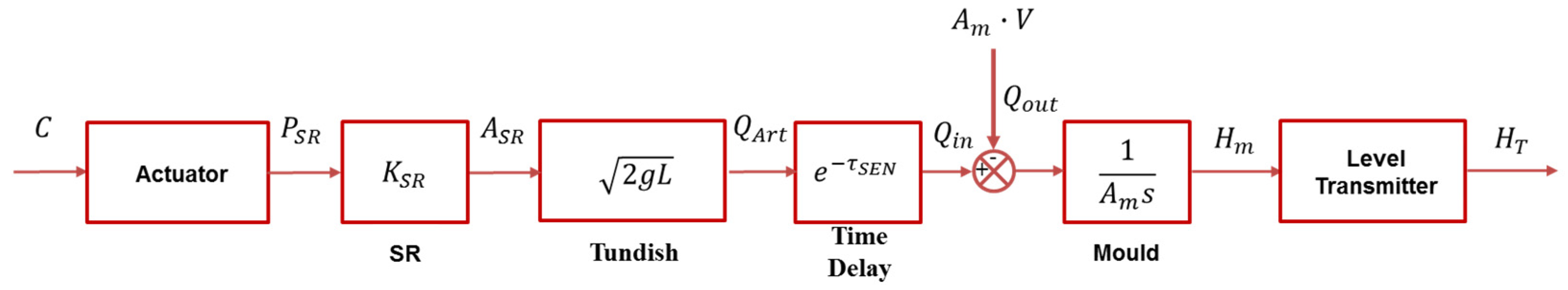
3. Control Structure

Here, a full model taking into account slow disturbances when using conventional control and the justification for the adaptive mold level control is presented.

3.1. Conventional Control

In [2,5] a simple model of the plant is presented and explained. It must be taken into account that SR and Tundish blocks in Figure 1 can slowly vary due to changes in the $K_{SR}$ gain of the valve caused by erosion or clogging and due to changes of $L$.

In this figure, the dynamics of the inlet flow $Q_{in}$ of the liquid steel to the mold is affected by the delay ${\tau }_{SEN}$ that can be identified. This is due to the transfer of the fluid by the Submerged Entry Nozzle (SEN) from the tundish to the liquid surface $H_m$ in the mold. The outflow $Q_{out}$ is determined by the product of $V$ and the cross section area $A_m$ of the casting product. Finally, the mold transfer function is an integrator whose gain is $1/A_m$.

In the continuous casting machine used in the case study in [2], the SR has a $K_{SR}^{°}=36 {\mathrm{mm}}^2/\mathrm{mm}$. The static characteristic of a new SR may vary during the casting, according to the physical–chemical conditions to which the valve is exposed [16]. Therefore, the SR gain uncertainty will be $K_{SR}\left(p_{SR}\right)=K_{SR}^{°}·∆K_{SR}\left(p_{SR}\right)$, where $∆K_{SR}\left(p_{SR}\right)$ has proportional relationships with the signal $P_{SR}$.

In the case study, to analyze the behavior of erosion and clogging, a total of 1127 carbon steel casts were selected corresponding to a semester of production. Their analysis was performed with the historical records of the Supervisory Control and Data Acquisition (SCADA) system. To this end, by means of scientific observation, an approximate value of the change in SR position in one hour was obtained for each steel cast. The relative time of $∆t=3600$ s was considered enough for diagnosing the slow disturbances in each cast and for compensation with an adaptive control approach. After examining the steel casts to determine the variation of the valve position from a reference instant, $-1\le ∆p_{SR}\le 1$ or $∆p_{SR}<-1$ or $∆p_{SR}>1$, the following results were obtained: a population of 925 normal casts, representing 82.07%; 160 casts with valve erosion, 14.2%; and 42 casts with valve clogging, 3.73%.

The SR clogging in the case study occurs mainly in steels with a chemical composition of higher aluminum content although other factors may influence this [4]. In such a case, material adherence occurs at the nozzle and/or the SR, which is evidenced in a trend of positive linear displacement $∆p_{SR-disp}>1$ of the valve operating area, as shown in the dashed straight line of Figure 2. From [16] and the analysis carried out in [5], it follows that this event includes the superposition of an upward shift of the working position $∆p_{SR-disp}>1$, plus another $∆p_{SR-gain}$ induced by a gain increase in the dynamic characteristic of the SR.

For all the steel casts selected with valve clogging, corresponding to values of $∆p_{SR}>1$, a similar procedure was carried out, corroborating that the tendency of the valve position change is always linear, obtaining regression adjustments between 72.61% and 96.62%. Depending on the continuous casting conditions at each plant, clogging/unclogging cycles also appeared, and the SR position signal could be a succession of ramps whose periods are random [4].

The SR erosion in the case study mainly occurs with low carbon steels, being rare when casting with higher oxygen content. The phenomenon is evidenced in a negative displacement trend $∆p_{SR}<-1$ of the valve operating area, as illustrated by the dotted straight line of Figure 3. From [16] and the analysis carried out in [5], it follows that this event includes the superposition of a downward shift of the working position $∆p_{SR}<-1$, plus another $∆p_{SR-gain}$ induced by an increase in the dynamic characteristic of the SR.

For all the steel casts selected with valve erosion, corresponding to values of $∆p_{SR}<-1$, a similar procedure was carried out, corroborating the tendency that the valve position change is always linear, obtaining regression adjustments between 62.3% and 97.6%.

By means of the sign of the $∆p_{SR}$ measurements in the case study, it was demonstrated that valve erosion and valve clogging are disturbances that do not occur in the same steel cast. Slow development events are also clear, as illustrated in Figure 2 and Figure 3. The variability in valve position changes were in the range $-23\le ∆p_{SR}\le 25$ for $∆t=3600$ s, which from a practical point of view was assumed to be related to the intensity levels of these events. In qualitative terms this could be classified, for example, as: low erosion, medium erosion, high erosion, low clogging, medium clogging and high clogging.

According to the above reasoning, during the valve erosion and valve clogging phenomena, the measurement of $∆p_{SR}$ reflects the superposition of two effects: as function $∆p_{SR-gain}$ dependent of $K_{SR}\left(p_{SR}\right)$, $∆v$ from a reference instant and $l$, plus another $∆p_{SR-disp}$. Therefore, in the model used in [5] for simulating purpose, it can be stated as:

$$∆p_{SR}=∆p_{SR-gain}+∆p_{SR-disp},$$

(1)

$$∆p_{SR-gain}=\frac{A_m·∆v}{\left(K_{SR}^{°}·∆K_{SR}\left(p_{SR}\right)\right)·\sqrt{2g·l}}.$$

(2)

The sense of (2) is implicit in the plant model illustrated in Figure 1, where $K_{SR}$ and $L$ can be variable parameters, although they vary more slowly than the plant dynamics. For all cases of valve erosion or valve clogging, it was assumed that $l=l^{°}=850$ mm and the value of $∆v$ is known from the measurements, which in the analyzed cases corresponds to $∆t=3600$ s. So, it can be noted that the multiplicative uncertainty $∆K_{SR}\left(p_{SR}\right)$ is an unknown parameter of (2).

However, empirical considerations were assumed from the determination of $∆K_{SR}\left(p_{SR}\right)$ in [5], in a model used for simulation purposes. The maximum value of the uncertainty $∆{\widehat{K}}_{SR-max}=6.8$ was obtained by increasing the parameter value until the MLC becomes unstable. It was also taken into account that when a critical case of erosion and clogging generates process shutdown, this occurs before the appearance of sustained level oscillations. Therefore, after analyzing the process signals for critical erosion and clogging cases, the upper values of $∆K_{SR}\left(p_{SR}\right)$ for $∆t=3600$ s were simulated with $∆{\widehat{K}}_{SR}\le 6$. Other cases with lower intensity of either valve erosion or clogging, such as $∆{\widehat{K}}_{SR}\in \left[1, 6\right]$, were also simulated heuristically assuming a linear interpolation of $∆p_{SR}$ versus $∆{\widehat{K}}_{SR}$, in correspondence with the value for each critical event in the case study.

Precisely due to the importance of good online compensation for slow disturbances, in the next section a solution for online identification of an estimated value of $∆{\widehat{K}}_{SR}$ with a greater precision than that achieved by the proposal made in [2,12] is presented.

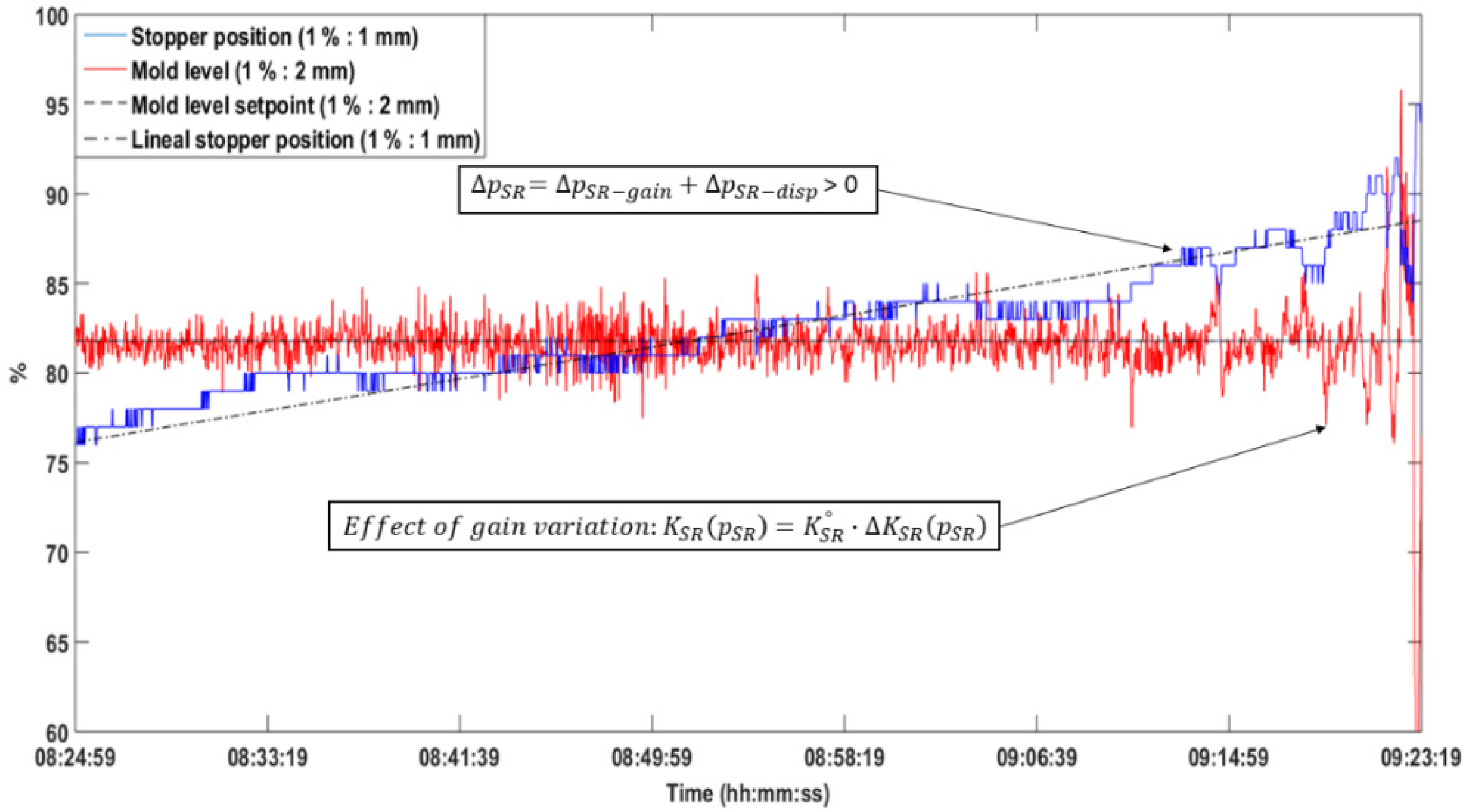
3.2. Adaptive Mold Level Control

An adaptive controller is a controller that can modify its behaviour in response to changes in the dynamics of the process and the character of the disturbances [17]. In this section, the adaptive control strategy of Figure 4 for dealing with slow disturbances in a MLC is described. It uses an adaptive controller that modifies the parameters of a Nonlinear PI on Robust Region (NPI-RR) control law, considering some parameter variations of the model used in its design [2].

Variations in $K_{SR}$ caused by erosion or clogging events, and the variation of $K_{Art}$ due to changes in $L$, produce slow changes in the value of the $K_p$ parameter corresponding to the Second Order Plus Delay Time (SOPTD) integrative model given in [2]. Focused on an adaptive control design, the following should be considered.

Control problem:

The Linear Time Invariant (LTI) model given in [2], under the condition that the plant gain varies much more slowly than the dynamics of the process, can be considered as a Linear Parameter Varying (LPV) System, such that:

$$P^{\prime }\left(s\right)=\frac{K_p\left(\rho \right)}{s\left(T_{p}s+1\right)}{e}^{-\tau s}=\frac{K_{SR}\left(P_{SR}\right)·K_{Art}\left(L\right)·K_m}{s\left(T_{p}s+1\right)}{e}^{-\tau s}.$$

(3)

The plant gain $K_p\left(\rho \right)$ varies as a function of $K_{SR}\left(P_{SR}\right)$, while $K_{SR}\left(P_{SR}\right)\in \left[K_{SR-min}, K_{SR-max}\right]$. The parameter $K_p\left(\rho \right)$ can also vary due to changes in $K_{Art}\left(L\right)=\sqrt{2g·L}$, which is determined by the variations of $L\in \left[L_{min}, L_{max}\right]$.

Control law:

The selection of the control law and the design of the adaptive law can be carried out separately, as for the Self-Tuning Regulator (STR).

The desired compensation can be achieved by multiplying the NPI-RR control law in [2] by an adaptation coefficient ${Coef}_{adapt}\left(\rho \right)$, inversely proportional to the change of $K_p\left(\rho \right)$. It follows that the adaptive control law can be considered as:

$$C^{\prime }\left(s\right)=C\left(s\right)·{Coef}_{adapt}\left(\rho \right).$$

(4)

Adaptive law:

The way to change controller gains, in correspondence with the parameter variations in the plant model, determines differences in each application. In this case, this can be done as follows:

$${Coef}_{adapt}\left(\rho \right)={Coef}_{SR}\left(P_{SR}\right)·{Coef}_{Art}\left(L\right),$$

(5)

where the term ${Coef}_{SR}\left(P_{SR}\right)$ will allow the compensation of the changes of $K_{SR}\left(P_{SR}\right)$, while the term ${Coef}_{Art}\left(L\right)$ has the purpose of modifying the controller gains following the variation of $K_{Art}\left(L\right)$.

The use of the gain scheduling technique for calculating the term ${Coef}_{Art}\left(L\right)$ is simple and was presented in [2]. Below is a proposal that combines artificial neural network, fuzzy logic and online identification for obtaining the term:

$${Coef}_{SR}\left(p_{SR}\right)=\frac{K_{SR}^{°}}{{\widehat{K}}_{SR}\left(p_{SR}\right)}\approx \frac{1}{∆K_{SR}\left(p_{SR}\right)}.$$

(6)

4. Neuro-Fuzzy System for Estimating Valve Gain

In this work the neuro-fuzzy system is used as a technique to fit a FIS from data or to enrich it through learning. For the design of the neural application the following basic steps were followed: (1) Problem statement; (2) System requirements; (3) selection of Artificial Neural Network (ANN) model; (4) Data available and selection of relevant input and output variables; (5) Selection of train, test and check data sets; (6) Data pre-processing; (7) Training process; (8) Use the model and evaluate its results.

(1)

Problem statement:

In [2] a fuzzy algorithm consisting of a zero-order Sugeno model for estimating the valve gain variations caused by erosion or clogging events was proposed. The estimator is as follows:

$${\widehat{K}}_{SR}\left(p_{SR}\right)\approx K_{SR}^{°}·∆K_{SR}\left(p_{SR}\right).$$

(7)

However, the accuracy of the inference system is based on, first, transforming human knowledge or experience of MLC with SR into the rule base and database of the fuzzy inference system; and, second, the heuristic tuning of membership functions so as to minimize the estimation error of ${\widehat{K}}_{SR}\left(p_{SR}\right)$.

(2)

System requirements:

To establish the system requirements, the desired error bound, the type of formulation to be applied, the available form of the data, the required time response, and the available or necessary computer equipment were proposed.

The data corresponding to the variables of interest, sampled every 1 s during the course of the steel casts with valve erosion and clogging events, were exported in csv files from the SCADA of the continuous casting machine. This form is compatible with the Microsoft Excel program and allows subsequent import from Matlab^®. To obtain the data $∆K_{SR}$, ${Coef}_{SR}$ corresponding to the adaptive control system proposed in [2], it was necessary to obtain them from the simulations carried out in Matlab^® with the model used in [5]. In this way, all the data of the process variables were completed in the form of matrices and vectors, saved in files with the extension “mat”.

In this work, a type of functional adjustment formulation is required for obtaining the function relationships among ${\widehat{K}}_{SR}\left(p_{SR}\right)$ and the selected input variables. The goal is to achieve training and test errors lower than 10% and deviations between process values and estimated values (root mean square error) ($RMSE$) lower than the largest obtained (for clogging: $RMSE=23.5$ and for erosion $RMSE=19.75$) with the FIS presented in [2].

In addition, for this application it is recommended to obtain initially an offline model without response time restrictions and with the use of conventional computing means. This will facilitate the implementation and updating of the model.

(3)

Selection of ANN model:

There are many types of network model [30]. The two aspects of the problem statement above, causing inaccuracy in the inference system presented in [2], can be improved with the advantages offered by the ANFIS architecture [18,19], with a relatively low effort. The fuzzy inference system may approximate any nonlinearity, but the learning ability and the relational structure of the artificial neural networks with the decision-making mechanism of the fuzzy logic are combined in ANFIS.

ANFIS realizes learning with samples, using a training data set as in artificial neural networks. When the learning with samples is completed, an appropriate ANN model is obtained. In this way, the most ideal ANFIS structure for solving the related problem [19] is obtained. In this paper the ANFIS structure consists of five layers, representing the fuzzy algorithm. This consists of a zero-order Sugeno model with two inputs, each one composed of five membership functions, and one output for the consequent of each rule. The twenty-five established rules in [2] were analyzed for simplification, eliminating all those lacking a physical sense.

To model the new FIS, the Fuzzy Logic toolbox of Matlab^® (R2015a edition) on a PC, with a compact structure tool to implement an ANFIS, was used. This has the ability to support the FIS previously designed in [2], which is a way to start the training with the previous knowledge of the application and of shortening the time needed to obtain the model. Another advantage is that the ANFIS also generates a FIS after each training session, which can be exported to facilitate simulations and implementation of the case study.

(4)

Data available and selection of relevant inputs and output variables:

In this application, batch learning is proposed, starting from the possibility offered by SCADA in a continuous casting machine for exporting data corresponding to sets of steel casts with valve erosion and clogging events of different intensity levels.

The selection of the input variables of the ANFIS in the case study corresponds to the same arguments of the proposals in [2]. Therefore, two input variables can be enough, where the first compact variable is defined as:

$${Changes}_{SR}=∆p_{SR}-\frac{A_m∆v}{{\widehat{K}}_{SR-ident}\left(p_{SR}\left(t_i\right)\right)·\sqrt{2g·l}}\approx ∆p_{SR-disp},$$

(8)

where ${\widehat{K}}_{SR-ident}\left(p_{SR}\left(t_i\right)\right)$ is made for $K_{SR}\left(p_{SR}\right)$ corresponding to $t_i$ instant of or otherwise the value $K_{SR}^{°}$, equivalent to the initial instant of casting.

The second input variable is obtained from online identification based on the frequency response of the process. With an SI-I algorithm [31], closed-loop identification as in [2] is possible, but in this work a half step of $H_{r-offset}=3\%$ from 0% to +3% around the reference value $H_r$ was used for obtaining similar results. However, to avoid unnecessary disturbances of $H_r$, online identification will be enabled only during erosion and clogging events with well-separated values of $∆p_{SR-disp}$. In [2], positive results are showed for obtaining (7) and (6) with the use of:

$${Gain}_{SR}=\{\begin{array}{c}{K}_{SR}^{°}, \forall t, t<t_1\\ {\widehat{K}}_{SR-ident}\left(p_{SR}\left(t_i\right)\right), \forall t, t_i\le t\le t_{i+1}\end{array},$$

(9)

where $i=1,\dots ,n$.

To define the universes of discourse of the input variables, a deep analysis of the process and the data, corresponding to numerous steel casts, was carried out. The emphasis was placed on including all possible real changes of the valve position and valve gain caused by erosion and clogging of the stopper valve, being the following, ${Changes}_{SR}\in \left[-25, 25\right] \mathrm{mm}/\mathrm{h}$ and ${Gain}_{SR}\in \left[36, 216\right] {\mathrm{mm}}^2/\mathrm{mm}$, in the case study.

The output variable range ${Coef}_{SR}\left(P_{SR}\right)\in \left[0.1666, 1\right]$ is obtained from (6), assuming $∆K_{SR}\left(p_{SR}\right)=∆{\widehat{K}}_{SR}\in \left[1, 6\right]$ for the case study.

(5)

Selection of training, test and check data sets:

The main condition to be taken into account for the selection of the data is that they should be a sufficiently representative number of all the situations and events that may occur [31]. Therefore, using an intentional sampling strategy as in [5], steel casts with different intensity levels of valve erosion and clogging events were selected. For organizing a process of linguistic classification of the intensity levels, subranges of the variable were heuristically defined, based on the calculation and analysis of the data of ${Changes}_{SR},$ as follows: Low erosion $-1<{Changes}_{SR}\le -7.92$; Medium erosion $-7.92<{Changes}_{SR}\le -15.3$; High erosion $-15.3<{Changes}_{SR}\le -25$ and Low clogging $1<{Changes}_{SR}\le 6.99$; Medium clogging $6.99<{Changes}_{SR}\le 15.99$; High clogging $15.99<{Changes}_{SR}\le 25$. The range $-1\le {Changes}_{SR}\le 1$ can be considered as a normal operating zone, free from erosion or clogging events.

From the previous classification, all the steel casts with different levels of valve erosion intensity were analyzed, selecting 24 steel casts (steel grades: FE500, SAE1039, SAE1018, SAE 1026, SAE 1022, SAE 1021 and FeE500S). From these only two had high valve erosion (7 and 24: FE500), seven were defined as being medium erosion (3, 6, 10, 13, 18, 20, 22) and 15 as low erosion (1, 2, 4, 5, 8, 9, 11, 12, 14, 15, 16, 17, 19, 21, 23). This proportion is representative of the incidence rate of each level of intensity of the event in the population selected for the case study.

Valve clogging occurred less frequently: in this case 16 steel casts were selected (steel grades: SAE 1026, SAE1018, SAE1023, SAE 1015, SAE 1022, FE 500 and SAE 1021); three with high clogging (1, 5, 6), three with medium clogging (2, 10, 14) and 10 with low clogging (3, 4, 7, 8, 9, 11, 12, 13, 15, 16), achieving similar rates to the real incidence in the case study. This selection process also took into account the criterion of including representatives of all the intensity levels of each event in the training, test and check sets.

After the selection process of all the patterns, they were divided into two groups: one more numerous with 75% of the data to carry out the learning process, as a result of the sum of 50% for the training set and 25% for testing. In this way, the ANFIS is trained using 12 erosion and eight clogging examples as a learning set, while the error made by the ANN model when applied to six erosion patterns and four clogging patterns is verified. The information contained in both sets is similar, thus enabling the proper use of the cross-validation technique [30]. 25% of the remaining data patterns (six erosion patterns and four clogging patterns) were reserved for the check set, allowing measuring the effectiveness of the new model in a completely objective way with representative events of all the situations that may occur.

(6)

Data pre-processing:

In this study, a set of input and output data has been prepared for developing the ANN model. To improve the training process of the model, all data need to be scaled before using them for modeling. The following scaling equations were used:

$${Changes}_{SRn}=\frac{{Changes}_{SR}}{\left|{Changes}_{SRmax}\right|},$$

(10)

$${Gain}_{SRn}=\frac{{Gain}_{SR}-{Gain}_{SRmin}}{{Gain}_{SRmax}-{Gain}_{SR-min}},$$

(11)

where ${Changes}_{SRn}\in \left[-1, +1\right]$ and ${Gain}_{SRn}\in \left[0, +1\right]$. The output variable ${Coef}_{SR}\left(P_{SR}\right)\in \left[0.1666, 1\right]$ is within $\left[0, +1\right]$ range.

(7)

Training process:

The training phase of the proposed model is implemented by means of the ANFIS training algorithms for Fuzzy Logic Toolbox in Matlab^® [32]. The selected data above of steel casts for training and testing sets and the previous FIS [2] must be loaded from the ANFIS Editor. The two available ANFIS parameter optimization method options must be proved: hybrid and backpropagation.

Normally, the ANFIS case must be tested with different methods and epochs, measuring the learning error and the generalization error, until the desired ones are reached. In the case of not obtaining acceptable results, some of the previous phases will have to be reviewed again: the training and test sets may not be representative, the variables may not have been chosen well, or they may not have been preprocessed or appropriately scaled.

The training process is terminated when any of the following conditions is satisfied: the maximum number of epochs is reached; the performance gradient falls below a minimum value; or the performance is minimized to the target value. As explained in the cross-validation method, there is no interest in prolonging the training indefinitely, as there comes a time when generalization is lost and the only data are memorized details (noise) of the learning set. The usual decision is to keep the model in the iteration for which the minimum error was obtained in the test set [30].

(8)

Use the model and evaluate its results:

Once the training phase is finished and the ideal FIS parameters have been stored, the ANFIS model is ready to be applied to new cases of steel casts for the checking set (not used in training) to measure its effectiveness in a completely objective way. If the results are obtained within the desired margin of error, then the new FIS can be used in the real work environment [30]. In order to illustrate the ANFIS model selected more intuitively, the adaptation subsystem applied for compensating slow disturbances of valve clogging and erosion on the mold level control is showed in Figure 5.

Taking into account that the model will be used for a complex and rigorous process, then it is also convenient to verify the accuracy of the established models for diagnosing the change of stopper rod using goodness-of-fit statistical parameters such as: $RMSE$, correlation coefficient ($R$) and the mean absolute percentage error ($MAPE$) [25,33].

The $RMSE$ can accurately measure the deviation between process values and estimated ones, and the $R$ is able to provide information on the strength of correlation between them. They are calculated using the following equation:

$$RMSE=\sqrt{\frac{1}{j}{{\displaystyle \sum }}_{i=1}^j{({\widehat{K}}_{SR}\left(\mathrm{i}\right)-K_{SR}\left(\mathrm{i}\right))}^2},$$

(12)

$$R=\frac{{{\displaystyle \sum }}_{i=1}^j\left({\widehat{K}}_{SR}\left(\mathrm{i}\right)-\overline{{\widehat{K}}_{SR}}\right)\left(K_{SR}\left(\mathrm{i}\right)-\overline{K_{SR}}\right)}{\sqrt{{{\displaystyle \sum }}_{i=1}^j{\left({\widehat{K}}_{SR}\left(\mathrm{i}\right)-\overline{{\widehat{K}}_{SR}}\right)}^2}\sqrt{{{\displaystyle \sum }}_{i=1}^j{\left(K_{SR}\left(\mathrm{i}\right)-\overline{K_{SR}}\right)}^2}},$$

(13)

where $\overline{K_{SR}}=\frac{1}{j}{{\displaystyle \sum }}_{i=1}^j{K}_{SR}\left(\mathrm{i}\right)$ and $\overline{{\widehat{K}}_{SR}}=\frac{1}{j}{{\displaystyle \sum }}_{i=1}^j{\widehat{K}}_{SR}\left(\mathrm{i}\right)$, respectively.

The $MAPE$ is used to measure the error between the estimated and the process values, and it particularly considers the ratio of error to the original values. The smaller the $MAPE$ value is, the higher the estimation accuracy is. The value of $MAPE$ is calculated by using the following equation:

$$MAPE=\frac{1}{j}{{\displaystyle \sum }}_{i=1}^j\left|\frac{{\widehat{K}}_{SR}\left(\mathrm{i}\right)-K_{SR}\left(\mathrm{i}\right)}{K_{SR}\left(\mathrm{i}\right)}\right|.$$

(14)

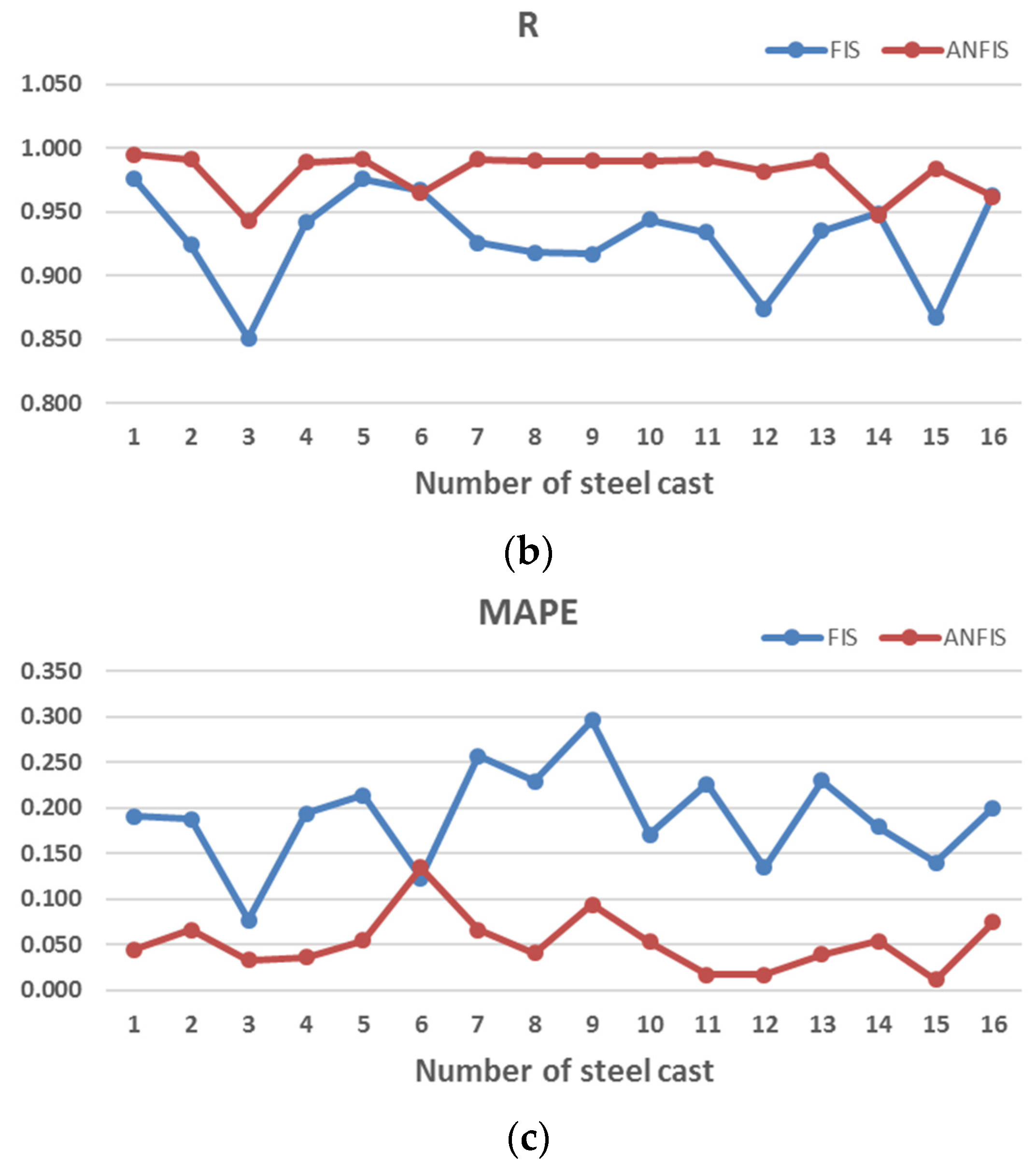
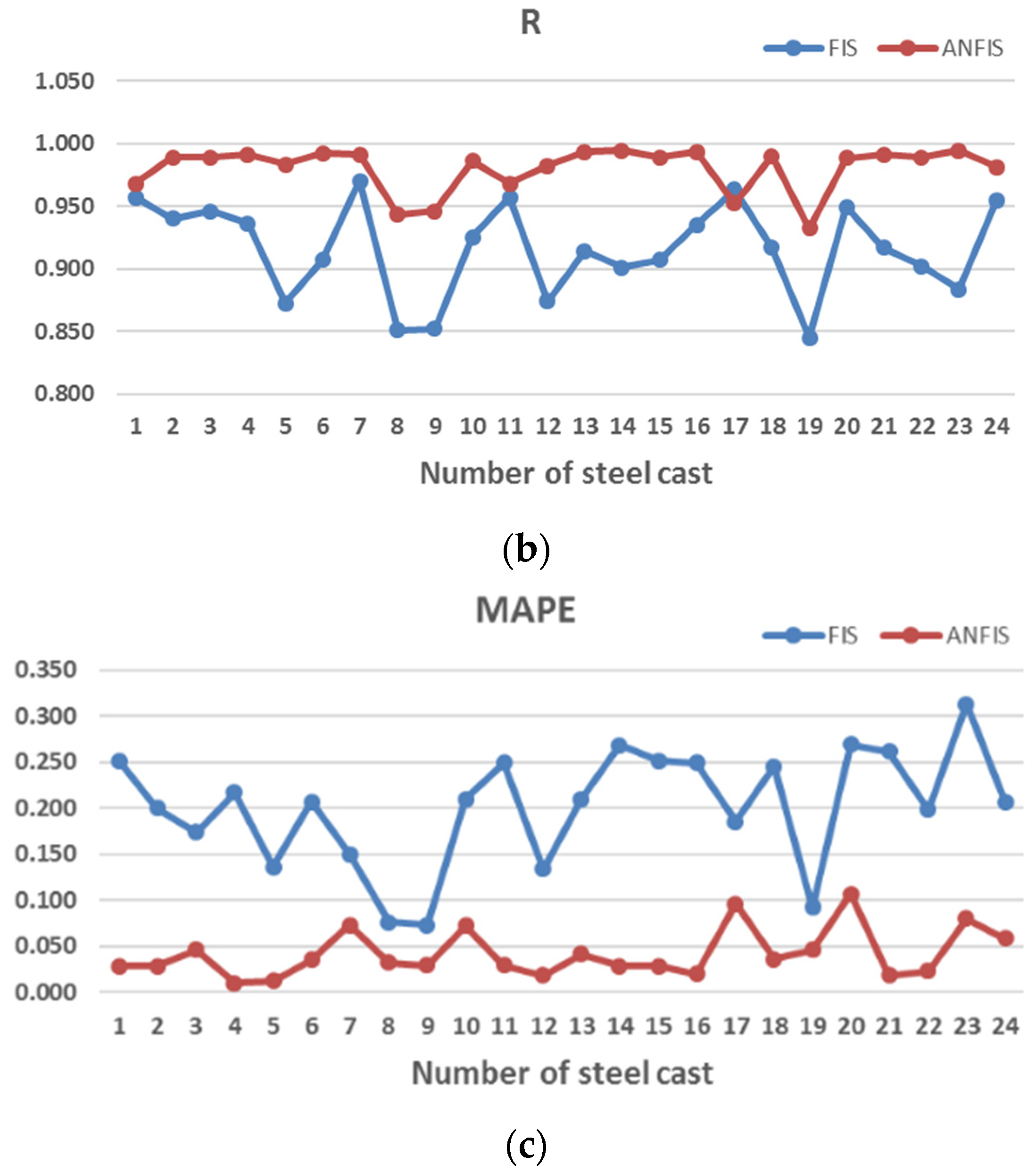
5. Results and Discussion

In this section, the results obtained when applying the previous developments are reported.

5.1. ANFIS Model Generation

The above steps for modeling the ANFIS were performed. The simplification of the reported twenty-five rules in [2] yielded nineteen established rules. The final version of the ANFIS model that will be presented resulted from several changes, training phases and analysis, until the desired system requirements were reached. The model was obtained using a computer with hardware Processor Intel^® Xeon^® CPU E5-2430 v2 @ 2.50 GHz (two processors), a RAM Memory of 16.0 GB and Operative System of 64 bit.

The best training phase, comparing hybrid and backpropagation ANFIS parameter optimization methods for FIS training, incrementing the epochs from 10 to 50 by steps of 10, are shown in

Table 3. The best training phase for obtaining the final Adaptive-Network-based Fuzzy Inference System (ANFIS) model.

Model Training	Epochs	Method	Simulation Time (hh:mm:ss)	Training Error (%)	Test Error (%)	Check Error (%)	Observations
1	10	Hybrid	0:06:59	3.6	3.9	6.1	Consequents out of ranges
2	10	Backpropagation	0:06:51	5.2	5.4	6.8	Well
3	20	Hybrid	0:13:52	3.5	3.7	6.3	Consequents out of ranges
4	20	Backpropagation	0:13:42	4.2	4.4	5.9	Well
5	30	Hybrid	0:20:47	3.3	3.6	6.2	Consequents out of ranges
6	30	Backpropagation	0:20:33	3.8	4	5.4	Well
7	40	Hybrid	0:27:24	2.9	3.8	7.2	Consequents out of ranges
8	40	Backpropagation	0:27:23	3.2	3.5	5	Well
9	50	Hybrid	0:34:23	2.7	3.6	9	Consequents out of ranges
10	50	Backpropagation	0:34:14	2.9	3.3	4.9	Well

.

Several changes for achieving acceptable results were proved. For example, the universe of discourse of ${Changes}_{SR}\in \left[-25, 25\right]$ provided better results than the previous ${Changes}_{SR}\in \left[-50, 50\right]$ used in [2]. This is reasonable because in the case study, ${Changes}_{SR}$ or $∆p_{SR-disp}$ satisfy that $-25\le ∆p_{SR-disp}\le 25$ for $∆t=3600$ s. Also, the empirical considerations assumed for upper values of $∆{\widehat{K}}_{SR}\in \left[5, 6\right]$ versus $∆t=3600$ s with critical erosion and clogging cases were proved. At this point a careful analysis of the process signals for these critical events and their physical interpretation, taking into account the typical behavior [16] of the relationship between $∆p_{SR-disp}$ versus $∆{\widehat{K}}_{SR}$, was realized. Finally, good results were obtained assuming $∆{\widehat{K}}_{SR}=5$ for the critical valve erosion case of steel cast number seven and $∆{\widehat{K}}_{SR}=6$ for the critical valve clogging case of steel cast number five. The cases with lower intensity of valve erosion or clogging were assumed by a linear interpolation of $∆p_{SR-disp}$ versus $∆{\widehat{K}}_{SR}$, proportionally to the value for each critical event.

The backpropagation ANFIS parameter optimization method with 50 epochs in 34 min and 14 s satisfied the system requirements of training and test errors lower than 10% and obtaining the best FIS training with the rules base shown in

Table 4. Rules base of the ANFIS model.

Coef-SR				Changes-SR
		EH	E	N	Cl	ClH
Gain-SR	Nominal	-	0.5494	0.9664	0.4821	-
	M	0.265	0.4185	0.746	0.4089	0.2877
	MH	0.2553	0.2739	0.956	0.2832	0.2779
	H	0.2091	0.2209	-	0.22	0.2271
	VH	0.1655	-	-	-	0.1737

. In this table, the symbols and respective membership functions (mf) are: Nom, with z mf; M, with pi mf; MH, with pi mf; H, with pi mf; VH, with s mf; N, with gauss mf; E, with pi mf; EH, with z mf; Cl, with pi mf; ClH, with s mf; Gain-SR is ${Gain}_{SR}$; Changes-SR is ${Changes}_{SR}$ and Coef-SR is ${Coef}_{SR}$.

The time consumed in the training phase indicates the possibility of considering a combined training of the model in a future implementation. This would be very convenient to keep the FIS updated with new real data from the process. The new data could be selected from the historic data base using a subroutine program in the SCADA. Besides, an interpolation of the identified values of the ${Gain}_{SR}$, as well as an analysis of the trade-off between the disturbing effects of a greater number of identification steps and the obtained accuracy, could be also considered.

5.2. Use of the ANFIS Model

The obtained ANFIS model and the previous FIS were used to compare the diagnostic accuracy of the change of stopper rod. This was realized at simulation scale with all selected data of valve erosion (24 steel casts) and valve clogging (16 steel casts), the same steel casts of the training, testing and checking sets.

The $RMSE$, $R$ and $MAPE$ obtained when using ANFIS and FIS models with all the steel casts in valve clogging are shown in Figure 6. The system requirement of $RMSE<23.5$ for the case of valve clogging using the ANFIS model was verified.

The ANFIS model allows a maximum value of $RMSE=13.66$ while the FIS gives $RMSE=23.5$ for the valve clogging cases. The mean average values of $\overline{RMSE}=4.29$ for ANFIS and $\overline{RMSE}=14.135$ for FIS were also obtained. Besides, for ANFIS, the values of $MAPE\le 0.13$ indicated a higher predictive accuracy and strong correlation, evident for all cases of $R$ close to 1.

Figure 7 shows the statistical parameters using ANFIS and FIS models with all steel casts in valve erosion. The system requirement of $RMSE<19.75$ for valve erosion using the ANFIS model was verified.

The maximum value of $RMSE=12.19$ for ANFIS, while it was $RMSE=19.75$ for FIS, and the mean average value of $\overline{RMSE}=3.31$ for ANFIS, while it was $\overline{RMSE}=13.68$ for FIS, obtained for the valve erosion cases. Besides, for ANFIS, the values of $MAPE\le 0.1$ indicates a higher predictive accuracy and strong correlation, evident for all cases of $R\ge 0.93$.

The above results mean that the ANFIS model presents smaller deviation between process values and estimated ones for valve clogging and valve erosion cases. Therefore, it is a good solution for improving the accuracy of the diagnostic and compensation of an adaptive MLC method for slow disturbances related to changes of stopper rod.

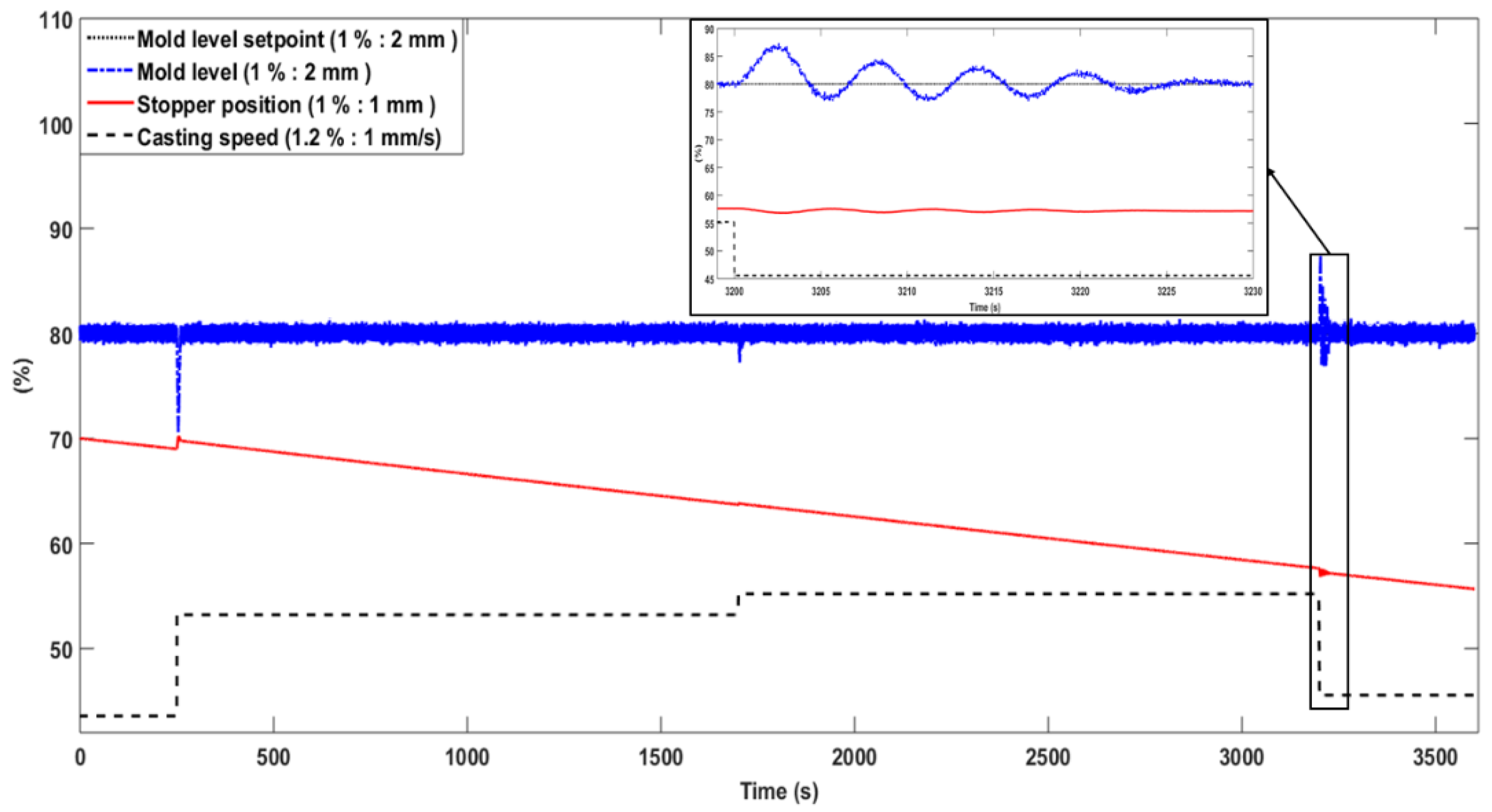
5.3. Neuro-Fuzzy Adaptive Mold Level Control Simulation

Here, in order to illustrate the performance of the adaptive mold level control of Figure 4 using the neuro-fuzzy model, four simulation experiments were realized. The good predictive accuracy of the ANFIS model and its impact for compensating for slow disturbances allowed a better tuning of the NPI-RR controller [2]. The goal was to achieve greater disturbance rejection with a robustness $M_s\in \left[2.0, 4.4\right]$, analyzing its trade off with the control effort to take care of the useful lifetime of the expensive SR mechanism, and the noise sensitivity.

The operation of the MLC of Figure 4 for steel cast number six with high valve clogging was simulated for a time $t=3600 \mathrm{s}$. At times $t=250, 1700, 3200 \mathrm{s}$ strong disturbances of casting speed increasing 8, 1.66 and decreasing 8 mm/s, were introduced, respectively. Also, an unclogging event was added at time $t=3400 \mathrm{s}$. Figure 8 and Figure 9 show the mold level performance with both neuro-fuzzy adaptive MLC and conventional MLC, in that order.

The operation of the MLC for steel cast number twenty with medium valve erosion was simulated for a time $t=3600 \mathrm{s}$, shown in Figure 4. At times $t=250, 1700, 3200 \mathrm{s}$ strong disturbances of casting speed increasing 8, 1.66 and decreasing 8 mm/s, were introduced, respectively. The mold level performance with neuro-fuzzy adaptive MLC and not adaptive MLC, are shown in Figure 10 and Figure 11.

The conventional mold level control shown in Figure 9 and Figure 11 has not diagnosed and compensated for slow disturbances related to SR changes. Those are the reasons for the unacceptable observed level fluctuations that could cause a high cost of casting interruptions, or several defects.

6. Conclusions

In this paper, an ANFIS model for improving the accuracy of the diagnosis, and compensation of an adaptive MLC method for slow disturbances related to changes of the stopper rod, is presented. In steel continuous casting several product defects are caused by mold level fluctuations. Level fluctuations are difficult to avoid in this complicated and multi disturbance process. The proposal presented here focuses on level fluctuations caused by erosion and valve clogging in mold level control systems using a stopper rod. The experiences of working in a steel plant for more than 20 years and the results of this work, which is part of ongoing research on the subject for almost the last decade, have provided evidence that this problem demands an adaptive control approach.

The ANFIS model for diagnosing and compensating for erosion and valve clogging is an effective solution as part of a second loop for adjusting the controller parameters in an adaptive MLC strategy. Two compact input variables, and their functional relationship with a compensation coefficient of the valve gain variations, could allow batch learning from historic data of the SCADA to be carried out. The results indicate that the model has high accuracy with the training, testing and checking sets. Additional evaluations using the statistical parameters: $RMSE$, $R$ and $MAPE$ with data from 40 steel casts perturbed by valve erosion and clogging of different intensity levels show very low deviations between process values and estimated values, as well as a strong correlation and a higher estimation accuracy.

In the future implementation of the proposed solution, a combined training of the model, which would be very convenient to keep the FIS updated with new data from the process, could be considered. Besides, an interpolation of the identified values of the SR gain could also be considered, as well as an analysis of the trade-off between the disturbing effects of a greater number of identification steps and the obtained accuracy.

References

1. Vynnycky, M. Continuous Casting. Metals 2019, 9, 643. [Google Scholar] [CrossRef] [Green Version]
2. Yero, G.G.; Mendoza, M.R.; Albertos, P. Robust nonlinear adaptive mould level control for steel continuous casting. IFAC-PapersOnLine 2018, 51, 164–170. [Google Scholar] [CrossRef]
3. Thomas, B.G. Review on modeling and simulation of continuous casting. Steel Res. Int. 2018, 89, 1700312. [Google Scholar] [CrossRef]
4. Jabri, K. Etude et Amélioration des Performances et de la Robustesse des lois de Commande de Procédés Sidérurgiques Application à la Régulation de Niveau en Coulée Continue. Ph.D. Thesis, Université Paris Sud-Paris XI, Orsay, France, 2010. [Google Scholar]
5. Yero, G.G. Modelado y Control de Nivel en un Molde de Vaciado Continuo. Ph.D. Thesis, Universidad de Oriente, Santiago de Cuba, Cuba, 2017. [Google Scholar]
6. Thomas, B.; Yuan, Q.; Zhao, B.; Vanka, S.P. Transient fluid-flow phenomena in the continuous steel-slab casting mold and defect formation. JOM-e 2006, 58, 16–36. [Google Scholar] [CrossRef]
7. Thomas, B.G. Fluid flow in the mold. Chapter 2003, 14, 14.1–14.41. [Google Scholar]
8. Camisani-Calzolari, F.; Craig, I.; Pistorius, P. A review on causes of surface defects in continuous casting. IFAC Proc. Vol. 2003, 36, 113–121. [Google Scholar] [CrossRef]
9. Thomas, B.G. On-line detection of quality problems in continuous casting of steel. In Modeling, Control and Optimization in Ferrous and Nonferrous Industry, Proceedings of the 2003 Materials Science and Technology Symposium, Chicago, IL, USA, 10–12 November 2003; TMS: Warrendale, PA, USA, 2003; pp. 29–45. [Google Scholar]
10. Bergman, L. Measurement Prediction and Control of Steel Flows in the Casting Nozzle and Mould. Master’s Thesis, Lulea University of Technology, Luleå, Sweden, 2006. [Google Scholar]
11. Kim, S.; Kim, J.; Kim, J.; Kim, J. Continuous Casting Technologies of Stainless Steel at POSCO Stainless Steelmaking Plant. In AISTech 2007 Proceedings; AIST: Warrendale, PA, USA, 2007; Volume 1, Available online: https://www.tib.eu/en/search/id/tema%3ATEMA20070803165/Continuous-casting-technologies-of-stainless-steel/ (accessed on 18 July 2020).
12. Popa, E.M.; Kiss, I. Assessment of surface defects in the continuously cast steel. Acta Tech. Corviniensis-Bull. Eng. 2011, 4, 109. [Google Scholar]
13. Zhang, H.; Wang, W. Mold simulator study of the initial solidification of molten steel in continuous casting mold: Part II. Effects of mold oscillation and mold level fluctuation. Metall. Mater. Trans. B 2016, 47, 920–931. [Google Scholar] [CrossRef]
14. De Keyser, R. Improved mould-level control in a continuous steel casting line. Control Eng. Pract. 1997, 5, 231–237. [Google Scholar] [CrossRef]
15. Schuurmans, J.; Kamperman, A.; Middel, B.; van den Bosch, P. Robust mould level control. In Proceedings of the 2005, American Control Conference, Portland, OR, USA, 8–10 June 2005; pp. 2040–2045. [Google Scholar]
16. Smutný, L.; Farana, R.; Víteĉek, A.; Kaĉmář, D. Mould Level Control for the Continuous Steel Casting. IFAC Proc. Vol. 2005, 38, 163–168. [Google Scholar] [CrossRef] [Green Version]
17. Åström, K.J.; Wittenmark, B. Adaptive Control, 2nd ed.; Dover Publications Inc.: Mineola, NY, USA, 2013. [Google Scholar]
18. Jang, J.-S. ANFIS: Adaptive-network-based fuzzy inference system. IEEE Trans. Syst. Man Cybern. 1993, 23, 665–685. [Google Scholar] [CrossRef]
19. Karaboga, D.; Kaya, E. Adaptive network based fuzzy inference system (ANFIS) training approaches: A comprehensive survey. Artif. Intell. Rev. 2019, 52, 2263–2293. [Google Scholar] [CrossRef]
20. Ghosh, I.; Chakraborty, N. An Artificial Neural Network Model for the Comprehensive Study of the Solidification Defects During the Continuous Casting of Steel. Comput. Commun. Collab. 2018, 6, 1–14. [Google Scholar]
21. He, F.; Zhang, L. Mold breakout prediction in slab continuous casting based on combined method of GA-BP neural network and logic rules. Int. J. Adv. Manuf. Technol. 2018, 95, 4081–4089. [Google Scholar] [CrossRef]
22. Abouelazayem, S.; Glavinić, I.; Wondrak, T.; Hlava, J. Adaptive Control of Meniscus Velocity in Continuous Caster based on NARX Neural Network Model. IFAC-PapersOnLine 2019, 52, 222–227. [Google Scholar] [CrossRef]
23. Song, G.W.; Tama, B.A.; Park, J.; Hwang, J.Y.; Bang, J.; Park, S.J.; Lee, S. Temperature Control Optimization in a Steel-Making Continuous Casting Process Using a Multimodal Deep Learning Approach. Steel Res. Int. 2019, 90, 1900321. [Google Scholar] [CrossRef]
24. Zou, L.; Zhang, J.; Liu, Q.; Zeng, F.; Chen, J.; Guan, M. Prediction of central carbon segregation in continuous casting billet using a regularized extreme learning machine model. Metals 2019, 9, 1312. [Google Scholar] [CrossRef] [Green Version]
25. Wang, Y.; Wu, X.; Li, X.; Xie, Z.; Liu, R.; Liu, W.; Zhang, Y.; Xu, Y.; Liu, C. Prediction and Analysis of Tensile Properties of Austenitic Stainless Steel Using Artificial Neural Network. Metals 2020, 10, 234. [Google Scholar] [CrossRef] [Green Version]
26. Furtmüller, C.; Colaneri, P.; Del Re, L. Adaptive robust stabilization of continuous casting. Automatica 2012, 48, 225–232. [Google Scholar] [CrossRef]
27. Cedillo, V.; Morales, R. Biased flows in slab moulds induced by slide gates. Part I: Experimental measurements and flow simulation. Ironmak. Steelmak. 2018, 45, 204–214. [Google Scholar] [CrossRef]
28. Shen, P.; Li, H.-X. The consistency control of mold level in casting process. Control Eng. Pract. 2017, 62, 70–78. [Google Scholar] [CrossRef]
29. Feng, Y.; Wu, M.; Chen, X.; Chen, L.; Du, S. A Fuzzy PID Controller with Nonlinear Compensation Term for Mold Level of Continuous Casting Process. Inf. Sci. 2020, 539, 487–503. [Google Scholar] [CrossRef]
30. Del Brío, B.M.; Molina, A.S. Redes Neuronales y Sistemas Difusos, 3rd ed.; Alfaomega Ra-Ma: Madrid, Spain, 2006. [Google Scholar]
31. Liu, T.; Gao, F. Industrial Process Identification and Control Design: Step-Test and Relay-Experiment-Based Methods; Springer Science & Business Media: London, UK, 2011. [Google Scholar]
32. MathWorks Fuzzy Logic Toolbox Documentation. Available online: https://www.mathworks.com/help/fuzzy/fuzzy.html (accessed on 18 July 2020).
33. Su, W.; Lei, Z.; Yang, L.; Hu, Q. Mold-level prediction for continuous casting using VMD–SVR. Metals 2019, 9, 458. [Google Scholar] [CrossRef] [Green Version]
Figure 1. Simple plant model.
Metals 11 00056 g001
Figure 2. Real data from a cast with stopper rod (SR) clogging in the case study.
Metals 11 00056 g002
Figure 3. Real data from a cast with SR erosion in the case study.
Metals 11 00056 g003
Figure 4. Mold level control (MLC) block diagram with robust nonlinear adaptive control.
Metals 11 00056 g004
Figure 5. Block diagram of the subsystem applied for compensating the stopper gain variations.
Metals 11 00056 g005
Figure 6. Measuring the diagnostic accuracy for all steel casts with valve clogging: (a) comparing R M S E parameter values obtained with fuzzy inference system (FIS) and ANFIS; (b) comparing R parameter values obtained with FIS and ANFIS; (c) comparing M A P E parameter values obtained with FIS and ANFIS.
Metals 11 00056 g006aMetals 11 00056 g006b
Figure 7. Measuring the diagnostic accuracy for all steel casts with valve erosion: (a) comparing R M S E parameter values obtained with FIS and ANFIS; (b) comparing R parameter values obtained with FIS and ANFIS; (c) comparing M A P E parameter values obtained with FIS and ANFIS.
Metals 11 00056 g007aMetals 11 00056 g007b
Figure 8. Simulation of adaptive mold level control for a cast with high SR clogging: (a) mold level performance; (b) diagnostic and compensation of process gain change by valve clogging.
Metals 11 00056 g008
Figure 9. Simulation of conventional mold level control for a cast with SR high clogging.
Metals 11 00056 g009
Figure 10. Simulation of adaptive mold level control for a cast with medium SR erosion: (a) mold level performance; (b) diagnostic and compensation of process gain change by valve erosion.
Metals 11 00056 g010
Figure 11. Simulation of conventional mold level control for a cast with medium SR erosion.
Metals 11 00056 g011