A Focus on Dynamic Modulus: Effects of External and Internal Morphological Features

Abstract

The present work examines the effects of external and internal morphological features on the dynamic elastic modulus and its measure. It consists of two parts. The first part considers the effect of geometrical features of probes and shows the key role of roughness as source of a systematic error leading to the underestimation of the Young’s modulus. The second one is focused on the effect of porosity. Several models which consider the porosity as an ideal regular microstructure and the relative equations describing the Young’s modulus vs. porosity have been reviewed and critically discussed. The values of the relative modulus E_r predicted by different models are similar for materials with low porosity (p < 0.2) and isolated pores whereas they strongly diverge if p > 0.2 and interconnected pores are present. Moreover, such models fail to describe the elastic behavior of materials correctly also with low porosity (p ≈ 0.1) such as sintered steels in the case of pores with a preferred orientation and an irregular shape.

1. Introduction

In industrial design, the knowledge of the elastic characteristics of materials is of great relevance. The Young’s modulus can be measured in different ways, among them the tensile test is the most used even if dynamic measurements are more precise and versatile. Dynamic tests are substantially of two types:

(i)

The material is tested by ultrasounds and from the measure of the speed υ they travel through the material it is possible to determine the dynamic modulus E according to the relation:

$$\upsilon =\sqrt{E/\rho }$$

(1)

being ρ the density;

(ii)

Dynamic modulus is determined from the resonance frequency f of probes with suitable geometry (reeds, wires, plates, etc.). The experiments can be carried out by means of different techniques involving a large range of frequencies from some tenths of Hz to GHz; more details about these techniques can be found in refs [1,2,3,4,5,6].

The results of dynamic tests can be affected by both external (geometrical irregularity and roughness) and internal (cracks and porosity) morphological features of the probes. Therefore, the knowledge of the effects of morphology on the modulus and its measure becomes important on one hand to investigate the defects and their evolution, on the other hand to correct raw data from experimental errors. The present work focuses its attention on these aspects and examines the following points:

• the effect of roughness and dimensional changes of probes on the value of dynamic modulus obtained in Mechanical Spectroscopy (MS) tests;
• the effect of porosity.

The first point has a practical use for experimental measurements but is commonly underestimated and few papers can be found in the literature. The second one has been extensively investigated owing to the industrial relevance of porous materials and the possibility of realizing today different pore shapes through additive manufacturing or other techniques. A couple of examples are given in Figure 1 showing a bio-compatible scaffold for cell growth fabricated by two-photon polymerization using a femtosecond pulsed laser (a) and a 3D-printed woodpile structure of PEGDA-575 (poly(ethylene glycol) diacrylate, M_n = 575 Da) by micro-stereolithography (b). However, the task is quite challenging and the results controversial due to the great variety of porous materials with different pore morphology (shape, size, and size distribution) and relative densities varying from some tens percent (foams) [7] to values very close to that of the bulk material (pore-free) typical of sintered metals.

To discuss these points, the Young’s modulus values predicted by several models were compared to MS experimental data collected by examining different metals (aluminum, Ni-base superalloy IN792, sintered steel). It is understood that the Young’s modulus denotes an interatomic bond strength and cannot be changed by the macroscopic defect-like pore, the modulus E in the paper refers the effective modulus which in dynamic measurements was determined from the expression:

$$E={\left(\frac{2\pi \sqrt{12}}{m^2}\right)}^2{f}^2\rho \frac{L^4}{h^2}\mathsf{\Omega }$$

(2)

where

$$\mathsf{\Omega }=1.000+6.585{\left(\frac{h}{L}\right)}^2$$

(3)

is a geometrical correction factor that becomes ≈ 1 if L/h > 20, m is a constant depending on the vibration mode, h the thickness of the probe, L its length, and ρ the density of the material. The results presented here were obtained by using bar-shaped probes (28 mm × 7 mm × 0.46 mm), mounted in cantilever, excited by flexural vibrations, and operating in conditions of resonance (resonance frequency in the range of kHz) under a 10⁻⁶ mbar pressure and at a strain amplitude of 10⁻⁶. The first vibration mode was used with m = 1.875 and Ω = 1 due to dimensions of probes (L/h ≅ 60). A single electrode is used to excite and reveal the probe vibrations. To excite the vibrations the electrode is parallel to the probe and a periodic voltage is applied while for the detection a capacitative method is used. The experimental apparatus automatically identify the response frequency and follow it if it changes, e.g., during heating. The apparatus employed in the experiments was an automated vibrating reed analyzer (VRA 1604, CANTIL s.r.l, Bologna, Italy) [8]. Some experiments were carried out at constant temperature, others at increasing temperature with a heating rate of 1 °C/min.

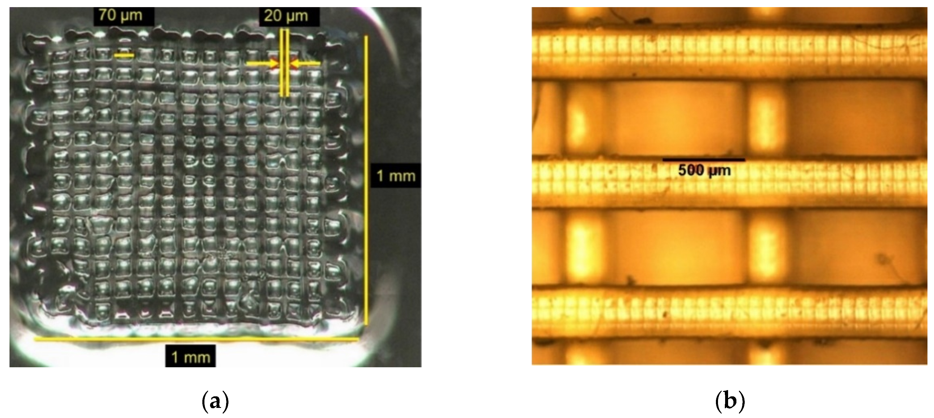
2. The Effect of Roughness, Shape Irregularity, and Dimensional Changes of Probes

The most adopted dynamic techniques for metallic materials are those of resonance. Such methodologies are in fact relatively fast and simple, non-destructive, allow the use of small probes, and offer the possibility to perform measurements in temperature. At the same time, however, they are sensitive to dimensional tolerances, are not easily applicable to some composites and require an a priori knowledge of some parameters of the material under examination. The evaluation of uncertainty is described in some papers (e.g., see [9,10]), even if such critical aspect is often neglected in industrial practice.

Dimensional accuracy, geometrical accuracy, and surface roughness are important issues and represent microscale deviations from the design of mechanical components. Shape irregularities are intrinsically connected to the way the probes are manufactured and described by tolerances. Roughness strongly depends on the history of the probes, namely the processes and treatments they undergo. It is commonly acknowledged its relevance in fatigue resistance [11] and corrosion behavior of metallic materials; however it is to the same extent important in dynamic modulus measurements.

Table 1. Indicative values of mean (Ra) and maximum (Rt) roughness due to different industrial processes.

Production Process	Ra (µm)			Rt (µm)
	Less Frequent	Common	Less Frequent
Metal Cutting
sawing	50–25	25–0.8	0.8–0.4	52
drilling	12.5–6.3	6.3–0.8	0.8–0.4	14
milling	25–6.3	6.3–0.5	0.5–0.12	14
Abrasive
grinding	6.3–1.6	1.6–0.05	0.05–0.012	4
electro-polishing	6.3–1.6	1.6–0.05	0.05–0.006	4
electrolytic grinding	1.6–1.64	1.64–0.1	0.1–0.05	4
polishing	1.6–0.4	0.4–0.05	0.05–0.006	1
lapping	1.6–0.2	0.2–0.012	0.012–0.006	1
Casting
sand casting	50–25	25–6.3	6.3–3.2	63
investment casting	6.3–3.2	3.2–1.6	1.6–0.4	11
die casting	3.2–1.6	1.6–0.8	0.8–0.4	6
Forming
hot rolling	50–25	25–12.5	12.5–3.2	75
forging	25–12.5	12.5–3.2	3.2–1.6	31
extruding	12.5–3.2	3.2–0.8	0.8–0.4	8
cold rolling, drawing	0.8–0.4	0.4–0.2	0.2–0.1	2
Other
electron beam cutting	–	6.3–0.4	0.4–0.2	14
laser cutting	–	6.3–0.4	0.4–0.2	14
EBM	12.5–3.2	3.2–0.8	0.8–0.4	9

reports the values of mean roughness (R_a) indicative of some industrial production processes [12] and clearly shows how extended is the variation range of roughness. The values of the maximum roughness (R_t) are determined by using conversion tables and considering a mean value of R_a.

To discuss how roughness, shape irregularities and dimensional changes of probes affect the dynamic measurements of the Young’s modulus E we will consider the simple case of a bar-shaped probe, mounted in cantilever and excited at the free end. Of course, the same considerations are valid for probes of different geometry (wires, plates etc.) and other experimental set-ups.

From Equation (2) resonance frequency f, thickness h and length L of the probe, and density ρ of the material are the factors affecting the errors in dynamic modulus measurements; they represent the source of the standard deviation u_c(E). Therefore, the variance is given by the expression:

$$u_c^2(E)={\displaystyle \sum _{i=1}^N{\left[\frac{1}{d_i}\frac{\partial E}{\partial x_i}u(x_i)\right]}^2}$$

(4)

where x_i are the causes of uncertainty, u(x_i) the respective standard deviations, d_i the coefficients which consider the distribution function associated with the terms x_i. Being the sensitivity coefficients c_i expressed by:

$$c_i=\frac{\partial E}{\partial x_i}\frac{x_i}{E}$$

(5)

Equation (4) can be re-written as:

$$u_c^2(E)=E^2{\displaystyle \sum _{i=1}^N{\left[\frac{1}{d_i}\frac{c_i}{x_i}u(x_i)\right]}^2}$$

(6)

In general, the contribution to the standard deviation due to frequency is low, of the order of ±0.002 Hz, since the precision provided by the instruments of common use is high. For what concerns the density, measurements employing the immersion method involve a value of u(ρ) of about ±0.01 g/cm³. The contributions that weigh most are those relating to length and thickness, since they appear in Equation (2) elevated to the fourth and second power, respectively.

In particular, roughness plays a key role in the measure of probe thickness since it introduces a systematic error leading to an overestimation of the h value and consequently an underestimation of the dynamic elastic modulus E: greater the roughness, lower the E value. In the case of a perfectly planar surface its profile corresponds to the baseline (y = 0) in Figure 2. Roughness involves the presence of peaks and valleys and the reference planes of the micrometer rest on the maximum ridges on both sides of the probe. Therefore, the instrument measures a value which is not the distance between the baselines on both sides of the probe (real thickness h) but that between the highest peaks. In fact, a systematic error which substantially corresponds to R_t is introduced and the measured value is h + R_t. Since L is usually much greater than h in this case the effect of roughness is lower.

The case of an aluminum probe manufactured by extrusion (R_t = 8 µm) will be examined as an example. The quantities appearing in Equation (2) are assumed to be uncorrelated and owing to the dimensions of the probe Ω = 1.

Table 2. Relevant values for the calculation of the dynamic modulus variance for an aluminum probe manufactured by extrusion (R_t = 8 µm).

Source of Uncertainty	u(xi)	Measured Mean Value xi	u(xi)/xi %	Probability Distribution	Divisor di	ci	(ci/di) [u(xi)/xi] %
Density ρ	±0.01 g/cm3	2.70 g/cm3	3.70 × 10−3	Rectangular	$\sqrt{3}$	1	2.14 × 10−3
Frequency f	±0.002 Hz	481.220 Hz	4.15 × 10−6	Rectangular	$\sqrt{3}$	2	4.80 × 10−6
Length L	±0.02 mm	27.80 mm	7.19 × 10−4	Rectangular	$\sqrt{3}$	4	1.66 × 10−3
Thickness h	±0.008 mm	0.460 mm	1.74 × 10−2	Rectangular	$\sqrt{3}$	2	2.01 × 10−2

reports the measured values of resonance frequency f, and the measured mean values of probe thickness h, probe length L and density of the material ρ together with the terms in Equation (6) which allows determining the standard deviation u_c²(E):.

$$u_c^2(E)=E^2\left[{\left(\frac{1}{\sqrt{3}}\frac{u(\rho )}{\rho }\right)}^2+{\left(\frac{2}{\sqrt{3}}\frac{u(f)}{f}\right)}^2+{\left(\frac{4}{\sqrt{3}}\frac{u(L)}{L}\right)}^2+{\left(\frac{2}{\sqrt{3}}\frac{u(h)}{h}\right)}^2\right]$$

(7)

The calculated mean values of the dynamic modulus and of the corresponding variance resulted in being E = 67.65 GPa and u_c(E) = 1.37 GPa, respectively.

As clearly emerges from this simple analysis, the term (c_i/d_i)[u(x_i)/x_i] that most affects u_c²(E) is that related to the thickness measurement. Moreover, the obtained mean value of E (67.65 GPa) is lower than the well-known and widely adopted mean value of aluminum Young’s modulus (69 GPa). This aspect should be stressed because current standards used in dynamic modulus measurements (e.g., E1876 – 15) do not mention roughness and its effect or they just point out that probes should have smooth and lapped surfaces and a standard technical finish to avoid an underestimation of the modulus.

Of course, the underestimation of Young’s modulus related to roughness depends on the thickness of the probe used in the experiments with increasing effects in thinner probes. To illustrate the concept Figure 3 displays the relative standard deviation u_c(E)/E vs. probe thickness for different values of R_t, corresponding to some industrial processes (see Table 1). The curves exhibit a decreasing trend as probe thickness increases.

In the case of probes manufactured by means of some very common industrial processes (hot rolling, sand casting, sawing, forging, etc.) roughness is so great that if the probe surface is not preliminarily submitted to mechanical and/or chemical polishing treatments, the error in the determination of Young’s modulus with 0.5 mm thick probes of common use can exceed 10%, which is absolutely unacceptable.

Since the relative roughness R_t/h is a parameter of fundamental importance for the error in dynamic modulus measurements Figure 4 shows how the relative standard deviation changes depending on R_t/h. The slope change for low R_t/h values is displayed in the frame.

Dynamic modulus measurements have a great advantage over quasi-static techniques (e.g., tensile tests) because they easily provide the evolution of Young’s modulus vs. temperature. The experiments are carried out by measuring the resonance frequency as the probe is heated and temperature increases at a constant rate. However, the determination of elastic modulus requires that the correct values of density, length, and thickness, namely those specific of each single temperature, are introduced into Equation (2). Unfortunately, it is not possible to measure these parameters during the test and the only available values are those measured at room temperature before mounting the probe in the vacuum chamber. Therefore, they must be corrected for the thermal expansion. Under the assumption of an isotropic expansion the correction is commonly done through the following expression including all the parameters:

$$E_T=E_0{\left(\frac{f_T}{f_0}\right)}^2\frac{1}{1+\alpha \Delta T}$$

(8)

where α is the thermal expansion coefficient, ΔT the difference between T and room temperature, E₀ and f₀ are modulus and resonance frequency at room temperature, E_T and f_T modulus and resonance frequency at the temperature T. As an example, Figure 5 shows the dynamic modulus vs. temperature of the IN792 superalloy with and without the correction described by Equation (8). The modulus variation due to the correction is small, slightly increases with temperature but remains of the order of 1% around 900 °C.

The results refer to an isotropic and homogeneous material; however they could change if it exhibits strong textures and/or microstructural features with a preferred orientation.

3. The Effect of Porosity

Danninger et al. [13] distinguished for sintered iron three main porosity p ranges: (i) p < 0.03 with fully isolated pores; (ii) p > 0.2 with interconnected pores of complex shape; (iii) porosity between 0.03 < p < 0.2 both isolated and interconnected pores are present in various amounts. Such approach is supported by a lot of experimental evidence. In Figure 6 the plot of different sintered steels, whose compositions are reported in

Table 3. Chemical compositions of the examined steels (MPIF Std. 35, [14]).

Steel	Chemical Composition wt. %
	Fe	C	Cu	Ni	Mo	Cr	Mn
F-0000	to balance	<0.3
F-0008	to balance	0.6 ÷ 0.9
FC-0200	to balance	<0.3	1.5 ÷ 3.9
FC-0205	to balance	0.3 ÷ 0.6	1.5 ÷ 3.9
FN-0200	to balance	<0.3	0.0 ÷ 2.5	1.0 ÷ 3.0
FN-0205	to balance	0.3 ÷ 0.6	0.0 ÷ 2.5	1.0 ÷ 3.0
FL-4405	to balance	0.4 ÷ 0.7			0.75 ÷ 0.95		0.05 ÷ 0.3
FL-5305	to balance	0.4 ÷ 0.6			0.40 ÷ 0.60	2.7 ÷ 3.3	0.05 ÷ 0.3
FLN2C-4005	to balance	0.4 ÷ 0.7	1.3 ÷ 1.7	1.55 ÷ 1.95	0.40 ÷ 0.60		0.05 ÷ 0.3

[14], is reported as an example: the trend exhibits a clear slope change for a porosity of about 20%. The discontinuity corresponds to a condition of prevalent interconnected pores.

Another relevant fact is that, differently from other elastic moduli, the relation between Young’s modulus and porosity is substantially independent of the Poisson’s ratio.

The relationships between elastic modulus and porosity found in the literature are quite various: in some cases, empirical equations have been proposed while in other ones they are derived from analytic treatments where pores are modeled either as spheroids or cubic cavities. In fact, today a general theory of pore shape effects is out of sight; however, some microstructures can be treated analytically.

Porous materials exhibit a large variety of pore shapes thus any model is indeed an idealization of the real microstructure; however, analytical treatments may be very useful to predict the elastic and plastic properties in some specific conditions. In a pioneering work Eudier [15] modeled the pores as small cylindrical cavities. Since then a lot of work has been made through both FEM simulations and analytic studies based on the theory of linear elasticity. Critical reviews of the results on the topic can be found in the papers of Moon [16] and Beiss [17]. Pores have been modeled by using different geometrical shapes (cylinders [15], rectangular parallelepipeds [18], etc.); however, the most common models are based on: (i) 3D arrangement of connected beams and (ii) spheroidal shape of pores. The expressions of E vs. porosity given by these models will be examined in the following and compared to experimental data regarding a sintered steel.

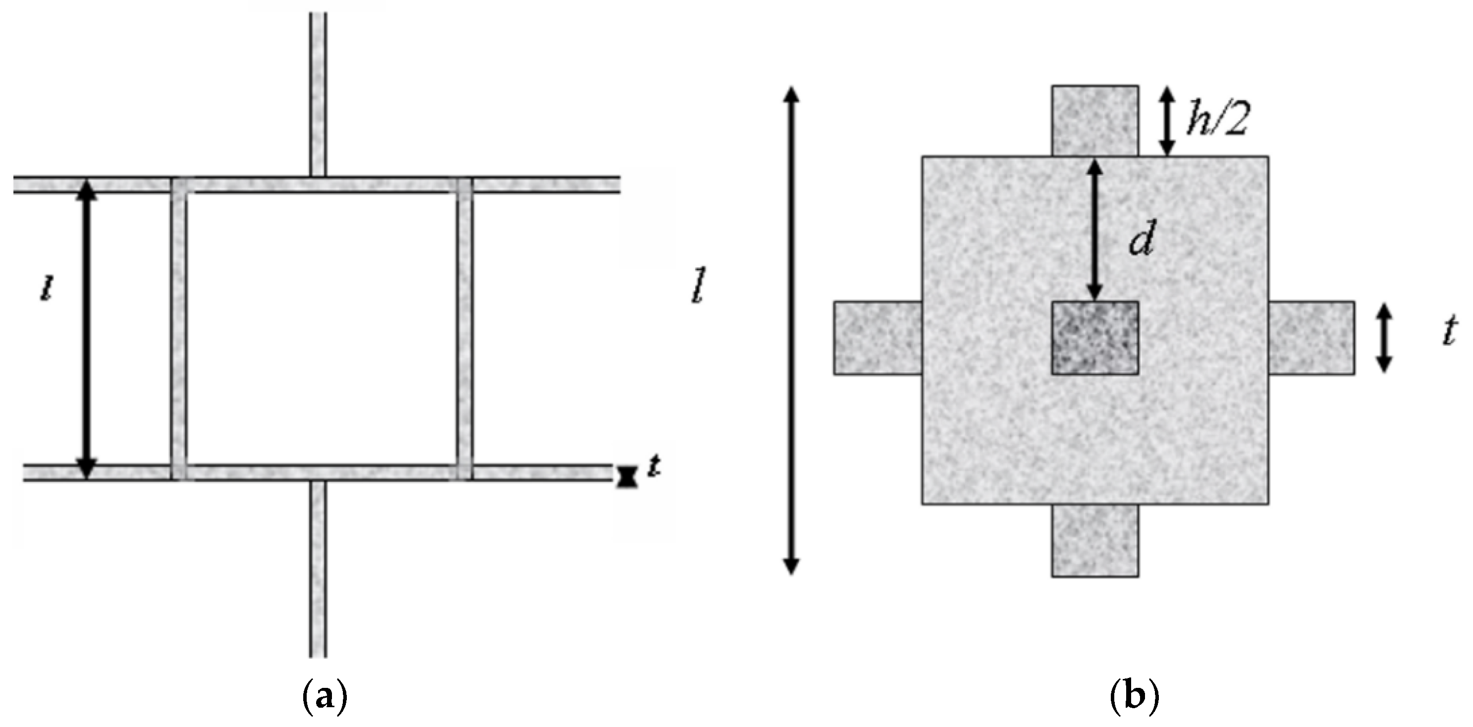
3.1. 3D Arrangement of Connected Beams

The most prominent example is the phenomenological model developed by Gibson and Ashby (GA) [19] to account for the mechanical characteristics of metal foams. It is based on the periodic 3D arrangement of connected beams with square cross section and large aspect ratio l/t (see Figure 7a).

Under the assumption that the structural elements behave as thin beams under three-point bending conditions [20] the model leads to a power law:

E ∝ ρ²

(9)

being E the Young’s modulus and ρ the relative density. The predictions of the model are in good agreement with experimental data in the case of foams with very small ligament junctions and ligament aspect ratios l/t ≥ 10; however significant deviations are observed in presence of massive nodes and ligaments [21], for instance those present in nano-porous materials.

The latter case has been examined by Pia and Delogu (PD) [22] who considered the nodes as cubic unit cells (see Figure 7b). The side of the node is l = (t + 2d + h) thus the foam density can be expressed as:

$$\rho ={\left(\frac{t}{l}+2\frac{d}{l}\right)}^3+3{\left(\frac{t}{l}\right)}^2\frac{h}{l}$$

(10)

which becomes the expression of the GA model if d → 0. The effective Young’s modulus E_eff results to be:

$$E_{eff}=\frac{8t^4}{l^2{h}^2}{\left[1+\frac{12+11\nu }{5}{\left(\frac{t}{h}\right)}^2\right]}^{-1}$$

(11)

where ν is the Poisson’s ratio. Experimental data of nano-porous materials are in good agreement with Equation (11) whereas relevant differences are observed when they are compared to the GA model relationship.

$$E_{eff}=\frac{t^4}{l^4}$$

(12)

3.2. Spheroidal Shape of Pores

The great advantage of the models which consider a spheroidal shape of pores (see Figure 8) consists of the possibility to describe spherical, disk-shaped, and needle-shaped pores through a single parameter, i.e., the aspect ratio, and in addition the local strain tensor is uniform within the pore [23].

In a material with a low pore content the uniform strain within the spheroidal pore can be used to find the elastic constants of the material; the analytical solution is due to Eshelby [23] and Wu [24] and it is noteworthy that an analytical solution is available only for spheroidal pores [25].

On the basis of Eshelby’s results, Krivoglaz and Cherevko [26] determined the following expression:

$$E_r=1-p\frac{3\left(1-{\nu }_0\right)\left(9+5{\nu }_0\right)}{2\left(7-5{\nu }_0\right)}$$

(13)

being E_r = E/E₀ the relative modulus, i.e., the ratio between the elastic modulus E of the porous material and the modulus E₀ of the same pore-free material, p = 1 − ρ the porosity (volume fraction of pores) and ν₀ the Poisson’s ratio of the pore-free material. In this treatment the pores are assumed to be spherical, of the same size and so diluted to neglect their interaction.

This approach has been improved by Vavakin and Salganik [27,28] who introduced in the model a size distribution of spherical pores of n different and increasing radii r_i and obtained the following expression:

$$E_r=E_0\left(1-2\pi \Omega \frac{\left(1-{\nu }_0\right)\left(9+5{\nu }_0\right)}{\left(7-5{\nu }_0\right)}\right)$$

(14)

The concentration parameter Ω = Nr³ depends the amount N of pores with radius r per unit volume. An extension of this model considers pore distributions defined as a discrete probability function f (r_i):

$$f_{\left(r_i\right)}=\frac{N_i}{{{\displaystyle \sum }}_{i=1}^n{N}_i}$$

(15)

The predictions of the extended model result in being in good agreement with experimental data for porous materials with isolated pores but not for materials with open pores or pores of irregular shape often observed in sintered metals where many pores tend to merge. Therefore, Manoylov et al. [29] presented a model considering merging and open pores that provides a better fitting of experimental data for a large variety of sintered materials. They used the theory of geometrical probabilities to estimate the number of pores that are close enough to merge and modeled the merging pores as ellipsoids of corresponding volume. In addition, the model has been implemented by considering the role of open pores. The volume fraction of open pores vs. the total volume of pores is determined and used to calculate the elastic modulus by assuming that the parts of the material containing open pores do not carry any load. The approach of Manoylov et al. [29] fits very well with experimental data for a large variety of sintered metals.

Boccaccini et al. [30] proposed an equation where the effective Young’s modulus is related to the porosity p and microstructural parameters such as axial ratio z/x of the spheroidal pores and their orientation (described by cos²α):

$$E_r={(1-p^{\frac{2}{3}})}^{1.21s}$$

(16)

with

$$s={\left(\frac{z}{x}\right)}^{1/3}\sqrt{1+{cos}^2\alpha \left[{\left(\frac{z}{x}\right)}^{-2}-1\right]}$$

(17)

The microstructural parameters involved in Equations (16) and (17) are directly obtained from microscopy observations and the relationship is valid in the whole range of porosity. Reference [30] reports an excellent agreement between model predictions and experimental data for many different materials. In the specific case of spherical pores (z/x) = 1 and cos²α = 0.33 thus s = 1 [31].

Other expressions have been proposed to correlate E_r and p; the most frequently used are:

(i)

the Maxwell-type approximation

$$E_{r }=\frac{1-p}{1+p}$$

(18)

(ii)

the self-consistent scheme approximation [32]

$$E_{r }=1-2p$$

(19)

(iii)

the power–law relation that can be derived via the Coble-Kingery approach [33]

$$E_{r }={\left(1-p\right)}^2$$

(20)

(iv)

the Spriggs equation [34] has been largely used and describes an exponential dependence of E_r to p where k is a fitting constant

$$E_{r }=\exp \left(-kp\right)$$

(21)

The main drawback of Equation (21) is that it does not consider a threshold porosity above which E_r becomes zero, as observed in many porous materials.

(v)

the Phani-Niyogi expression [35,36] where p* is a critical porosity at which E_r becomes zero and f a parameter that depends on pore morphology

$$E_{r }={\left(1-\frac{p}{p^{*}}\right)}^f$$

(22)

The percolation theory [37] predicts f = 2.1 for 3D porous materials; however experimental data are often well fitted by lower values approximately in the range 1.10–1.70. Lam et al. [38] suggested f = 1.

(vi)

Equation (23) was proposed by Pabst and Gregorová [39,40]; the value E_r predicted by this relationship approaches zero if p → p* and 1 if p → 0, namely it correctly corresponds to the physical bound conditions.

$$E_{r }=exp{\left(E^{*}-\frac{p}{1-\frac{p}{p^{*}}}\right)}^{}$$

(23)

The intrinsic modulus E* = lim_p→0 (E_r − 1)/p.

Figure 9 shows the trends of the aforesaid expressions.

From the plot in Figure 9 it is evident that the different models predict similar values of E_r for materials with low porosity: for p < 0.2 the modulus scattering is within 7%. If p > 0.2 the data resulting from different expressions strongly diverge, e.g., at p = 0.45 the E_r values cover a range of about 30%. The result is compatible with the presence of interconnected pores, as discussed by Danninger et al. [13].

Recently, an important contribution to the study of elastic modulus-porosity relation has been given by Pabst and Gregorová [41] who demonstrated that the Eshelby–Wu coefficients of Young’s modulus can be described by a unique function of the aspect ratio of pores with spheroidal shape and implemented in different models (Maxwell, self-consistent, power law and their model). They found that irrespectively of the model into which the Eshelby–Wu coefficients are implemented, Young’s modulus is weakly affected by prolate pores whereas it is reduced by oblate pores.

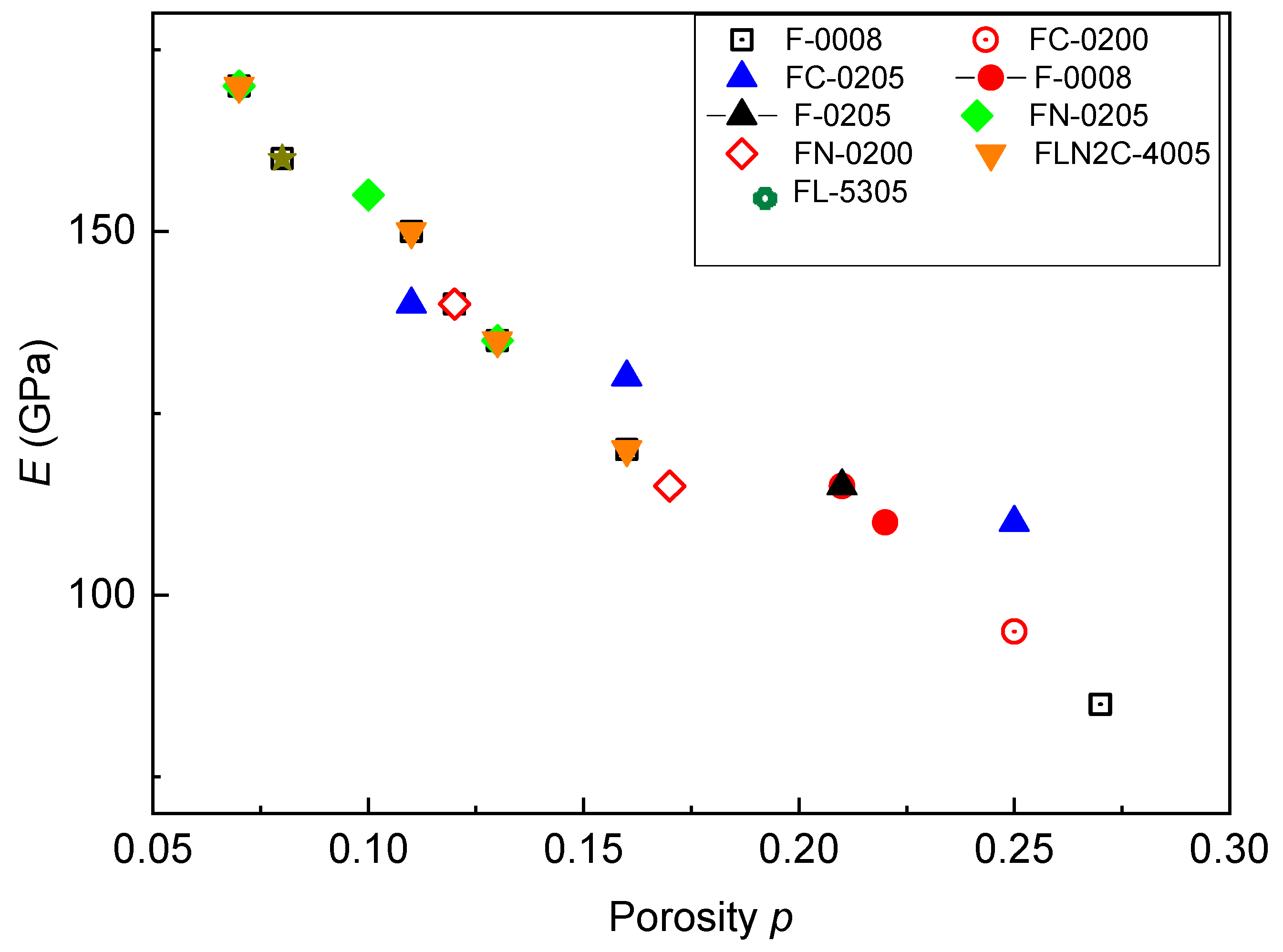
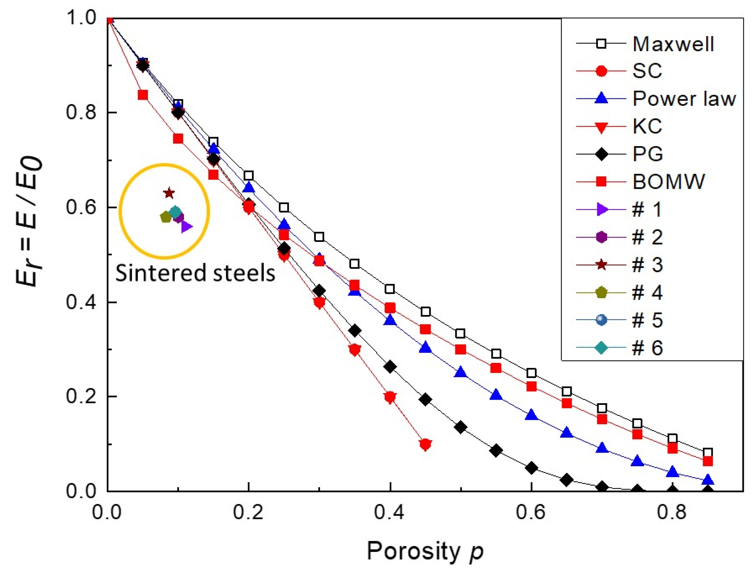
3.3. Prediction of Models and Elastic Behavior of Sintered Steels

Many metallic materials of great industrial interest, such as sintered steels, commonly exhibit low porosity (p < 0.2) but irregular and oriented pores (e.g., see Figure 10). Therefore, it is interesting to assess whether the models describing the Young’s modulus trend based on simple geometrical pore shapes can be used for describing their elastic properties. To this scope dynamic modulus measurements have been carried out on one of them (Fe-1.5Mo-0.5 C wt%) and the results compared to the values of the curves are shown in Figure 9.

The reeds for dynamic modulus measurements were cut from disks of a sintered steel in two different directions (parallel and perpendicular to the pressing axis). The steel has been sintered in H₂ atmosphere in three different conditions: (1) 1160 °C for 30 minutes; (2) 1160 °C for 30 min plus 1250 °C for 45 min; (3) 1160 °C for 30 min plus 1250 °C for 90 min. Therefore, we have examined six types of probes representative of three sintering processes and two orientations with respect the axis of disks; the measurements have been carried out on eight probes of each type and the mean values of porosity p and the relative modulus E_r are reported in

Table 4. Porosity p and relative modulus E_r of the steel sintered in three different conditions. The reeds have been cut in two different directions, parallel and perpendicular to the disk axis.

Samples		Porosity p	E/E0
# 1	1160 °C–30 min/Parallel	0.11 ± 0.01	0.56 ± 0.02
# 2	1160 °C–30 min/Perpendicular	0.10 ± 0.01	0.58 ± 0.02
# 3	1160 °C–30 min/1260 °C–90 min/Parallel	0.09 ± 0.03	0.63 ± 0.02
# 4	1160 °C–30 min/1260 °C–90 min/Perpendicular	0.08 ± 0.03	0.58 ± 0.04
# 5	1160 °C–30 min/1260 °C–45 min/Parallel	0.10 ± 0.01	0.59 ± 0.01
# 6	1160 °C–30 min/1260 °C–45 min/Perpendicular	0.10 ± 0.03	0.59 ± 0.02

and plotted in Figure 8.

Independently on the specific sintering treatment and the direction they were cut, all the probes have a similar porosity (~10%) consisting of isolated pores which represent the condition where the examined models provide quite similar results. Despite the low porosity (p < 0.2) Figure 8 clearly shows that there is a significant difference (~20%) between experimental data and the relative moduli E_r foreseen by the models. A similar discrepancy is observed for the sintered steels whose Young’s modulus is plotted in Figure 5. By taking E₀ = 210 GPa the relative modulus E_r also for these materials is always lower with respect to the values predicted by various models. Therefore, caution should be used in adopting the equations described in the previous section for predicting the elastic behavior of materials with pores of irregular shape such as sintered steels. In such cases a different approach to find E_r may be considered by means of FEM simulations based on the 3D reconstruction of real spatial microstructures. For instance, this method was successfully used by Chen et al. [42] for calculating the elastic moduli of porous La_0.6Sr_0.4Co_0.2Fe_0.8O_{3_δ} ceramic films. Today tomography techniques employing either X-ray or FIB/SEM are a powerful tool to characterize the inner morphology of solid bodies [43], reconstruct the 3D structure and supply the basic information for FEM analysis.

4. Conclusions

The effects of material external and internal morphological features on the dynamic elastic modulus and its measure have been examined and discussed. The results are summarized in the following.

(i)

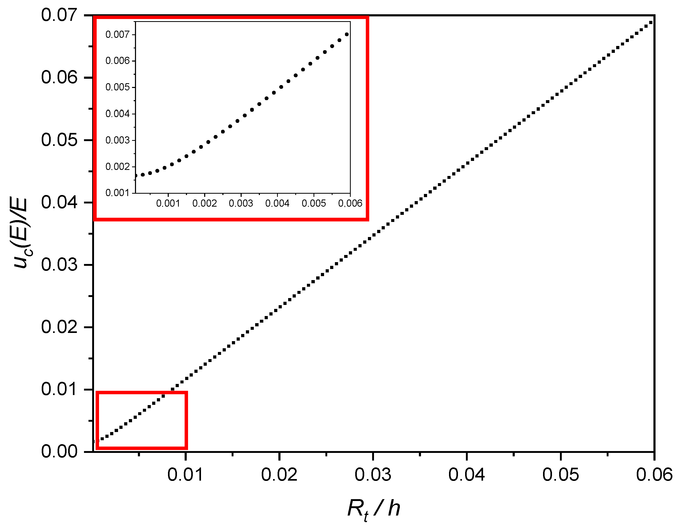
Probe roughness is the main source of uncertainty in dynamic modulus measurements. It involves a systematic error in the thickness measurement that leads to the underestimation of the modulus and its effect increases as the thickness of the probe decreases.

(ii)

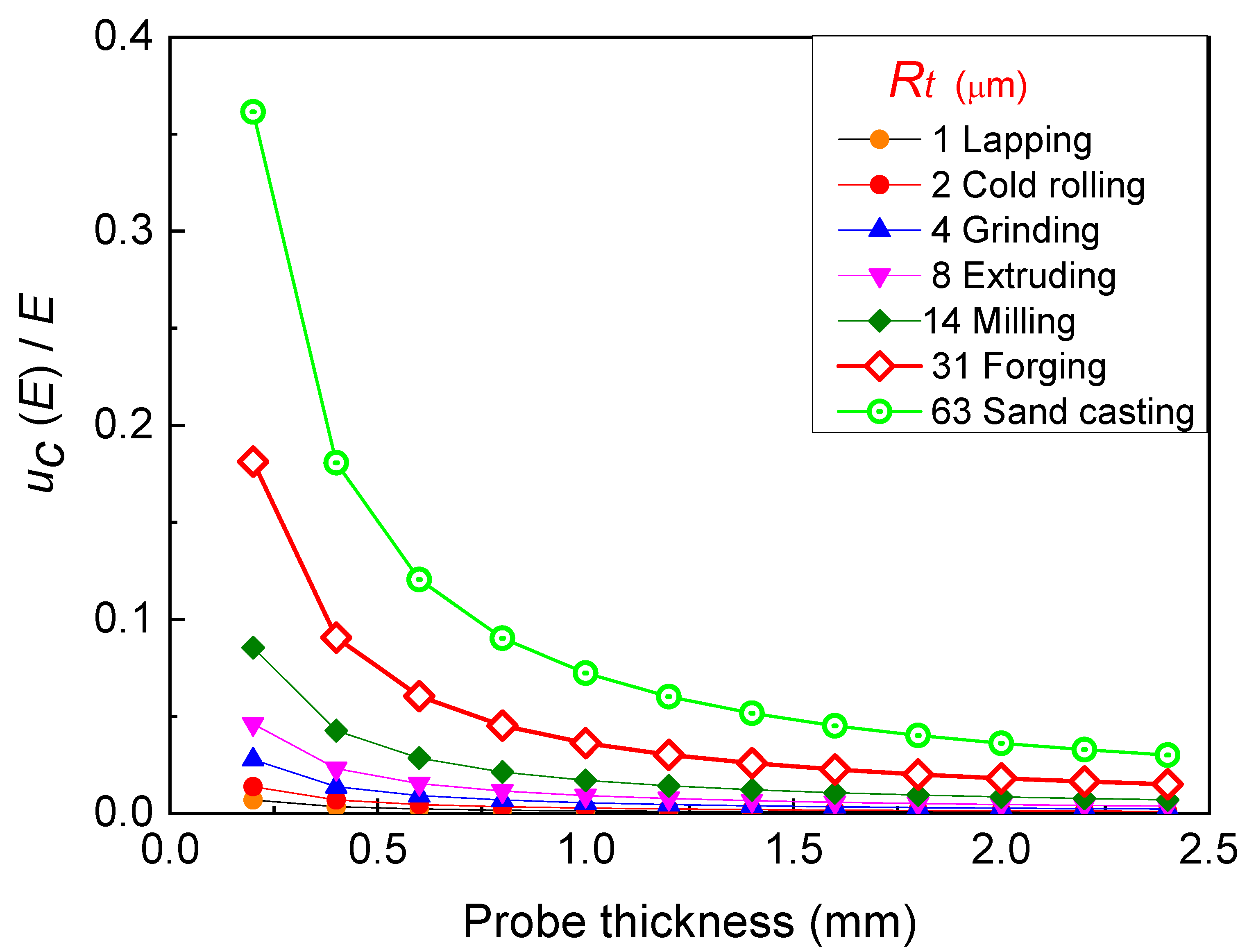
The analysis of the relative standard deviation u_c(E)/E depending on the probe thickness shows that for thicknesses of the order of 0.05 mm (commonly used in tests) it can exceed 10% in the case of probes produced through some conventional industrial processes (sawing, sand casting, hot forging, etc.). Therefore, it is of utmost importance a careful preparation of the surface to reduce the roughness as much as possible as stated by the standards. Nevertheless, an analysis of the roughness effect seems mandatory to estimate the standard deviation.

(iii)

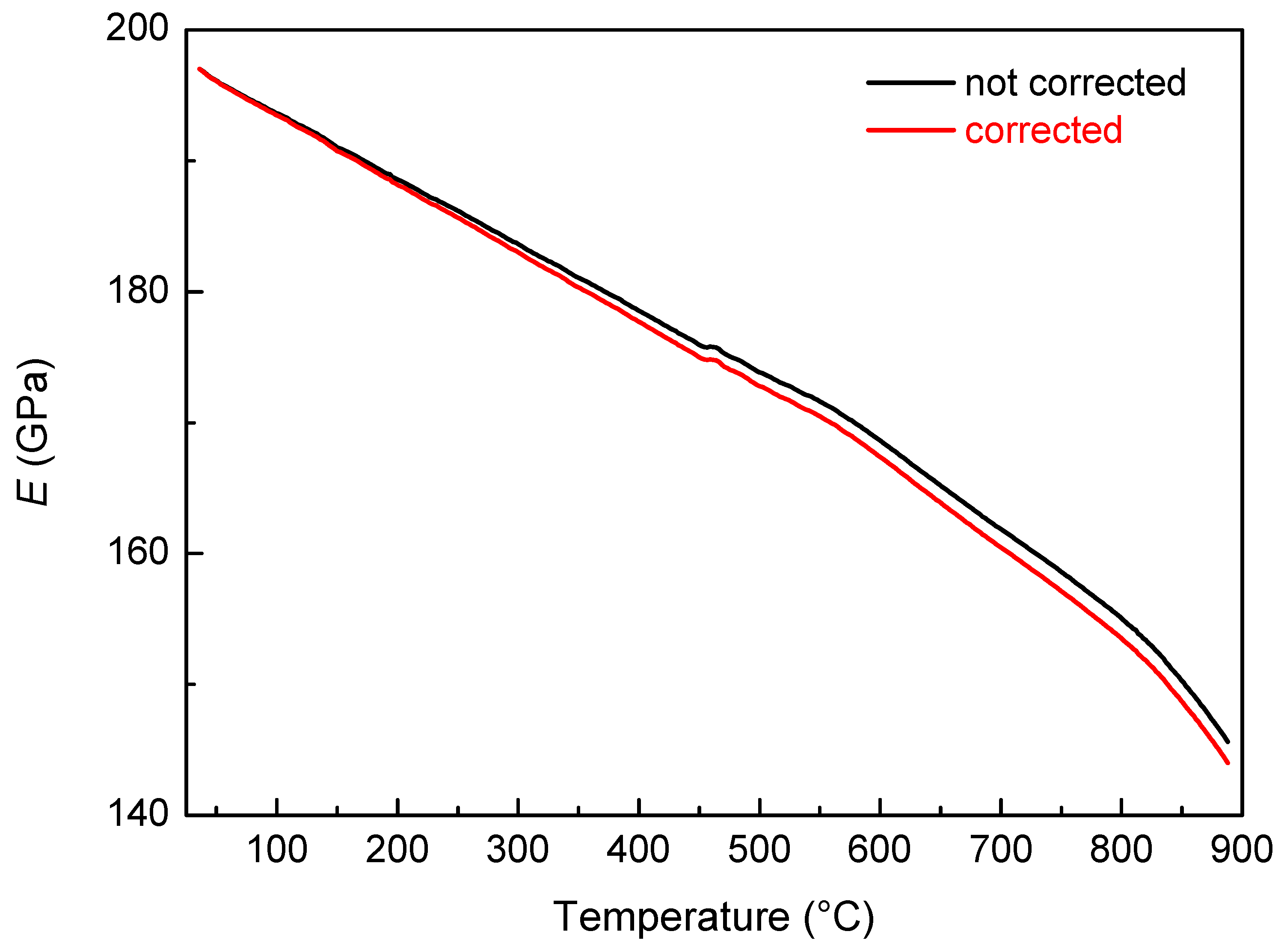
Data obtained by tests carried out in temperature need to be corrected from thermal expansion of the probe; however the error is small (<1% for temperature variations of about 900–1000 °C).

(iv)

The work examined several equations proposed in the literature to relate Young’s modulus of porous materials to porosity. These are mainly based on the modeling of porosity as an ideal regular microstructure and predict similar values of the relative modulus E_r for materials with low porosity (p < 0.2) whereas when p > 0.2, namely in presence of interconnected pores, data from different expressions strongly diverge. Moreover, also with low porosity (~10%) the comparison of experimental data obtained from a steel sintered with irregular and oriented pores shows significant deviations from the values predicted by these models. This is a further limit to the applicability of the examined equations.

(v)

In the case of materials with irregular shape of pores a different approach may be considered by means of FEM simulations based on the 3D reconstruction of real spatial microstructures obtained from tomography techniques employing either X-ray or FIB/SEM.

References

1. Nowick, A.S.; Berry, B.S. Anelastic Relaxation in Crystalline Solids; Academic Press: New York, NY, USA; London, UK, 1972. [Google Scholar]
2. Lakes, R.S. Viscoelastic Solids; CRC: Boca Raton, FL, USA, 1999. [Google Scholar]
3. ASTM E1876. Standard Test Method for Dynamic Young’s Modulus, Shear Modulus and Poisson’s Ratio by Impulse Excitation of Vibration; ASTM International: West Conshohocken, PA, USA, 2015. [Google Scholar] [CrossRef]
4. ASTM E1875. Standard Test Method for Dynamic Young’s Modulus, Shear Modulus and Poisson’s Ratio by Sonic Resonance; ASTM International: West Conshohocken, PA, USA, 2020. [Google Scholar] [CrossRef]
5. Wolfenden, A.; Harmouche, M.R.; Blessing, G.V.; Chen, Y.T.; Terranova, P.; Dayal, V.; Kinra, V.K.; Lemmens, J.W.; Phillips, R.R.; Smith, J.S.; et al. Dynamic Young’s modulus measurements in metallic ma-terials: Results of an interlaboratory testing program. J. Test. Eval. 1989, 17, 2–13. [Google Scholar] [CrossRef]
6. Roebben, G.; Bollen, B.; Brebels, A.; Van Humbeeck, J.; Van Biest, O. Impulse excitation apparatus to measure reso-nant frequencies, elastic moduli, and internal friction at room and high temperature. Rev. Sci. Instrum. 1997, 68, 4511–4515. [Google Scholar] [CrossRef]
7. Costanza, G.; Gusmano, G.; Montanari, R.; Tata, M.E.; Ucciardello, N. Effect of powder mix composition on Al foam morphology. J. Mater. Des. Appl. 2008, 222, 131–140. [Google Scholar] [CrossRef]
8. Amadori, S.; Campari, E.G.; Fiorini, A.L.; Montanari, R.; Pasquini, L.; Savini, L.; Bonetti, E. Automated resonant vibrating reed analyzer apparatus for a non destructive characterization of materials for industrial applications. Mater. Sci. Eng. A 2006, 442, 543–546. [Google Scholar] [CrossRef]
9. Birch, K. Estimating uncertainties in testing. In Measurement Good Practice Guide No. 36; Addison-Wesley Publishing Company, Inc.: London, UK, 2001. [Google Scholar]
10. Jurowski, K.; Grzeszczyk, S. Non-destructive method of concrete compressive strength determine based on dynam-ic Young’s modulus. In Monografie Technologii Betonu; Stowarzyszenie Producentów Cementu: Kraków, Poland, 2016; Volume 2, pp. 567–579. [Google Scholar]
11. Montanari, R.; Sili, A.; Costanza, G. Improvement of the fatigue behaviour of an Al6061/20%SiCp composite by means of Titanium coatings. Compos. Sci. Technol. 2001, 61, 2047–2054. [Google Scholar] [CrossRef]
12. DeGarmo, E.P.; Black, J.T.; Kohser, R.A. Materials and Process in Manufacturing; John Wiley & Sons: Hoboken, NJ, USA, 2003; p. 227. [Google Scholar]
13. Danninger, H.; Jangg, G.; Weiss, B.; Stickler, R. Microstructure and mechanical properties of sintered iron. Part I: Basic considerations and review of literature. Powder Metall. Int. 1993, 25, 170–219. [Google Scholar]
14. MPIF Standard 35. Materials Standards for PM Structural Parts, Rev. 2009; Metal Powder Industries Federation: Princeton, NJ, USA, 2009. [Google Scholar]
15. Eudier, M. The mechanical properties of sintered low-alloy steels. Powder Metall. 1962, 9, 278–290. [Google Scholar] [CrossRef]
16. Moon, J.R. Elastic moduli of powder metallurgy steels. Powder Metall. 1989, 32, 132–139. [Google Scholar] [CrossRef]
17. Beiss, P. Landolt Bōrnstein, Group VIII: Advanced Materials and Technologies. In Powder Metallurgy Data; Part 1: Metals and Magnets; Springer: Berlin/Heidelberg, Germany; New York, NY, USA, 2003; Volume 2. [Google Scholar]
18. Bocchini, G.F.; Montanari, R.; Varone, A. Influence of probe test orientation, sintering degree and morphological anisotropy of porosity on the Young’s modulus of homogeneous sintered steel. In Proceedings of the EPMA 2013, Gothenburg, Sweden, 15–18 September 2013. [Google Scholar]
19. Gibson, L.J.; Ashby, M.F. Cellular solids. In Structure and Properties, 2nd ed.; Cambridge University Press: Cambridge, UK, 1989. [Google Scholar]
20. Timoshenko, S.; Goodier, J. Theory of Elasticity, 3rd ed.; McGraw-Hill Book Company: New York, NY, USA, 1970. [Google Scholar]
21. Liu, R.; Antoniou, A. A relationship between the geometrical structure of a nanoporous metal foam and its modulus. Acta Mater. 2013, 61, 2390–2402. [Google Scholar] [CrossRef]
22. Pia, G.; Delogu, F. On the elastic deformation behavior of nanoporous metal foams. Scr. Mater. 2013, 69, 781–784. [Google Scholar] [CrossRef]
23. Eshelby, J.D. The determination of the elastic field of an ellipsoidal inclusion, and related problems. Proc. R. Soc. Lond. A 1957, 241, 376–396. [Google Scholar]
24. Wu, T.T. The effect of inclusion shape on the elastic moduli of a two-phase material. Int. J. Solids Struct. 1966, 2, 1–8. [Google Scholar] [CrossRef]
25. Torquato, S. Random Heterogeneous Materials—Microstructure and Macroscopic Properties; Springer: New York, NY, USA, 2002; pp. 437–563. [Google Scholar]
26. Krivoglaz, M.A.; Cherevko, A. On the elastic moduli of a solid mixture. Fiz. Met. Metalloved. 1959, 8, 161–164. [Google Scholar]
27. Vavakin, A.S.; Salganik, R.L. Effective characteristics of nonhomogeneous media with isolated non-homogeneities. Mech. Solids 1975, 10, 65–75. [Google Scholar]
28. Vavakin, A.S.; Salganik, R.L. Effective elastic characteristics of bodies with isolated cracks, cavities, and rigid non-homogeneities. Mech. Solids 1978, 13, 87–97. [Google Scholar]
29. Manoylov, A.V.; Borodich, F.M.; Evans, H.P. Modelling of elastic properties of sintered porous materials. Proc. R. Soc. A 2013, 469, 1–19. [Google Scholar] [CrossRef]
30. Boccaccini, A.R.; Ondracek, G.; Mazilu, P.; Windelberg, D. On the Effective Young’s Modulus of Elasticity for Po-rous Materials: Microstructure Modelling and Comparison between Calculated and Experimental Values. J. Mech. Behav. Mater. 1993, 4, 119–128. [Google Scholar] [CrossRef]
31. Ondracek, G. The Quantitative Microstructure Field Property Correlation of Multiphase and Porous Materials. Rev. Powder Metall. Phys. Ceram. 1987, 3, 205–322. [Google Scholar]
32. Markov, K.Z. Elementary Micromechanics of Heterogeneous Media. In Heterogeneous Media, Modeling and Simu-Lation in Science, Engineering and Technology; Markov, K., Preziosi, L., Eds.; Spinger Birkhäuser: Boston, MA, USA, 2000; p. 119. [Google Scholar]
33. Coble, R.L.; Kingery, W.D. Effect of porosity on physical properties of sintered alumina. J. Am. Ceram. Soc. 1956, 39, 377–385. [Google Scholar] [CrossRef]
34. Spriggs, R.M. Expression for Effect of Porosity on Elastic Modulus of Polycrystalline Refractory Materials, Particu-larly Aluminum Oxide. J. Am. Ceram. Soc. 1961, 44, 628–629. [Google Scholar] [CrossRef]
35. Phani, K.K.; Niyogi, S.K. Young’s modulus of porous brittle solids. J. Mater. Sci. 1987, 22, 257–263. [Google Scholar] [CrossRef]
36. Kovačik, J. Correlation between Young’s modulus and porosity in porous materials. J. Mater. Sci. Lett. 1999, 18, 1007–1010. [Google Scholar] [CrossRef]
37. Sahimi, M. Applications of Percolation Theory; Taylor & Francis: London, UK, 1994; p. 185. [Google Scholar]
38. Lam, D.C.; Lange, F.F.; Evans, A.G. Mechanical Properties of Partially Dense Alumina Produced from Powder Compacts. J. Am. Ceram. Soc. 1994, 77, 2113–2117. [Google Scholar] [CrossRef]
39. Pabst, W.; Gregorova, E. Mooney-type relation for the porosity dependence of the effective tensile modulus of ceramics. J. Mater. Sci. 2004, 39, 3213–3215. [Google Scholar] [CrossRef]
40. Pabst, W.; Gregorová, E. Effective elastic properties of alumina–zirconia composite ceramics—Part II: Microme-chanical modeling. Ceram. Silik. 2004, 48, 14–23. [Google Scholar]
41. Pabst, W.; Gregorová, E. Young’s modulus of isotropic porous materials with spheroidal pores. J. Eur. Ceram. Soc. 2014, 34, 3195–3207. [Google Scholar] [CrossRef]
42. Chen, Z.; Wang, X.; Giuliani, F.; Atkinson, A. Microstructural characteristics and elastic modulus of porous solids. Acta Mater. 2015, 89, 268–277. [Google Scholar] [CrossRef] [Green Version]
43. Maire, E.; Withers, P. Quantitative X-ray tomography. Int. Mater. Rev. 2014, 59, 1–43. [Google Scholar] [CrossRef] [Green Version]
Figure 1. (a) Bio-compatible PEGDA scaffold for cell growth fabricated by two-photon polymerization using a femtosecond pulsed laser. (b) 3D-printed woodpile structure of PEGDA-575 by micro-stereolithography.
Metals 11 00040 g001
Figure 2. Schematic view of a rough surface.
Metals 11 00040 g002
Figure 3. Trend of uc(E)/E vs. probe thickness h for given values of Rt.
Metals 11 00040 g003
Figure 4. Trend of uc(E)/E vs. Rt/h. In the frame the slope change for lower Rt/h values is displayed.
Metals 11 00040 g004
Figure 5. Comparison between dynamic modulus vs. temperature with (red line) and without (black line) thermal expansion correction.
Metals 11 00040 g005
Figure 6. Elastic modulus vs. porosity redrawn from ref. [14].
Metals 11 00040 g006
Figure 7. Interconnected thin beams form the cubic structure underlying the GA (a) and PD (b) models.
Metals 11 00040 g007
Figure 8. Spheroid with aspect ratio oa/oc.
Metals 11 00040 g008
Figure 9. Trends of Er vs. porosity p calculated with the following expressions: Maxwell-type approximation, self-consistent (SC) approximation, power law, Krivoglaz and Cherevko (KC), Pabst and Gregorova (PG), and Bocaccini et. al. (BOMW) in the specific case of spherical pores.
Metals 11 00040 g009
Figure 10. Typical structure of a sintered steel with pores of irregular shape.
Metals 11 00040 g010