Article

Discovery of New Ti-Based Alloys Aimed at Avoiding/Minimizing Formation of α” and ω-Phase Using CALPHAD and Artificial Intelligence

Multidisciplinary Analysis, Inverse Design, Robust Optimization and Control (MAIDROC) Laboratory, Department of Mechanical and Materials Engineering, Florida International University, Miami, FL 33174, USA
*
Author to whom correspondence should be addressed.
Metals 2021, 11(1), 15; https://doi.org/10.3390/met11010015
Submission received: 28 November 2020 / Revised: 18 December 2020 / Accepted: 19 December 2020 / Published: 24 December 2020
(This article belongs to the Special Issue Titanium and Its Alloys for Biomedical Applications)

Abstract

:
In this work, we studied a Ti-Nb-Zr-Sn system for exploring novel composition and temperatures that will be helpful in maximizing the stability of β phase while minimizing the formation of α” and ω-phase. The Ti-Nb-Zr-Sn system is free of toxic elements. This system was studied under the framework of CALculation of PHAse Diagram (CALPHAD) approach for determining the stability of various phases. These data were analyzed through artificial intelligence (AI) algorithms. Deep learning artificial neural network (DLANN) models were developed for various phases as a function of alloy composition and temperature. Software was written in Python programming language and DLANN models were developed utilizing TensorFlow/Keras libraries. DLANN models were used to predict various phases for new compositions and temperatures and provided a more complete dataset. This dataset was further analyzed through the concept of self-organizing maps (SOM) for determining correlations between phase stability of various phases, chemical composition, and temperature. Through this study, we determined candidate alloy compositions and temperatures that will be helpful in avoiding/minimizing formation of α” and ω-phase in a Ti-Zr-Nb-Sn system. This approach can be utilized in other systems such as ω-free shape memory alloys. DLANN models can even be used on a common Android mobile phone.

1. Introduction

Titanium-based alloys have been widely accepted for biomedical applications due to comparatively superior biocompatibility and anti-corrosion properties [1,2,3,4,5]. Efforts are being made to explore new alloys that contain elements that are not toxic, as well as develop alloys with Young’s modulus comparable to human bone to avoid stress shielding [2]. Young’s modulus (YM) of common implant materials varies between 100–230 GPa, which is significantly higher when compared with that of bone, which is between 10 and 40 GPa [1]. This difference in YM results in non-uniform distribution of stress in the implant materials and the surrounding bone structure. This can result in the failure of an implant [1]. Titanium alloys containing β-phase as the predominant phase are known to have lower values of Young’s modulus [2,3,4,5,6,7,8,9]. Thermodynamically, α and β are stable phases, while α” and ω-phase are metastable phases [2]. Composition and processing of alloys play an important role in determining the concentrations of various phases, which directly affect mechanical properties of these alloys [6,7,8,9].
During processing or heat-treatment of Ti-based alloys, they are subjected to cooling from an elevated temperature at various cooling rates [10,11,12,13,14]. The cooling rate can affect the stability of β-phase and it can transform into α, α˝ or ω-phase, while ω-phase can also form isothermally during ageing [12]. Among these phases, ω-phase possesses the highest modulus value. Precipitation of α and ω-phase can result in an increase in the Young’s modulus of the alloy [12,13]. Regarding α”-phase, it is a desired phase in shape memory alloys [12]. In Ti-based biomaterials, precipitation of α, α˝ or ω-phase can lead to degradation of mechanical properties, specifically Young’s modulus [2,10,11,12,13,14]. In titanium alloys, experiments show that ω-phase can be stabilized and has been observed at cryogenic temperatures [15]. From first-principle calculations, researchers have demonstrated the scope of development of ω-phase free Ti-Ta-X shape memory alloys [16].
In this work, we chose the Ti-Nb-Zr-Sn system, which is free of toxic chemical elements [17] such as aluminum [18] and vanadium [19]. Niobium is a strong β-phase stabilizer [9]. In the presence of Nb, Zr also becomes a strong β-phase stabilizer [1]. Additionally, Nb and Zr are biocompatible and demonstrate excellent resistance to corrosion [20]. Sn is also biocompatible and has been used as an alloying element in small amounts [21]. The addition of Sn leads to a decrease in elastic modulus of Ti-based biomaterials [22]. Sn addition can help in suppressing precipitation of α˝ and ω-phase for lower and higher cooling rates, respectively [22]. One of the aims is to optimize the alloy composition so that an optimum amount of Sn addition can prove to be beneficial in the lowering of the elastic modulus and in the suppression of precipitation of α˝ and ω-phase [22].
The Ti-Nb-Zr-Sn system was studied under the framework of CALculation of PHAse Diagram (CALPHAD) approach through Thermo-Calc software [23]. It was used for determining concentrations of various stable and metastable phases for a large set of compositions and temperatures, and thus generating a dataset suitable enough for applying artificial intelligence (AI) algorithms, including deep learning [24] and self-organizing maps (SOM) [25]. These data were then used for developing deep learning artificial neural network (DLANN) models for various phases as a function of alloy composition and temperature. Software for developing the DLANN model was written in Python programming language using TensorFlow [26] and Keras [27] libraries. DLANN models were used as a predictive tool for predicting the concentrations of metastable phases for new compositions and temperatures. This resulting dataset was then analyzed by the concept of self-organizing maps (SOM) [25] for determining various patterns and correlations within the dataset among alloying elements, temperatures, and stable and metastable phases.
Through this work, we were able to identify the composition and temperature regimes that will provide ω-phase free Ti-based alloys with a minimal amount of α” phase. We have reported chemical compositions of several candidate alloys along with temperatures that will be helpful in achieving ω-phase free Ti-based alloys (Ti-Nb-Zr-Sn system). Our research team has significant experience in designing alloys by application of artificial intelligence (AI) algorithms on data generated from experiments and data generated under the framework of the CALPHAD approach. We have successfully designed titanium alloys [28], aluminum alloys [29,30], hard magnets (AlNiCo) [31,32], soft magnets (FINEMET type) [33,34], and Ni-based superalloys [35]. Thus, we propose this computational design approach, which can be easily adopted in other alloy systems and can help in developing ω-phase free Ti-based biomaterials with improved mechanical properties.

2. Materials and Methods

As mentioned, we chose the Ti-Nb-Zr-Sn system for this work. Bounds for concentrations for each of the four alloying elements were defined on the basis of available literature [1,2,3,4,5,6,7,8,9,10,11,12,13,14,15,16,17,18,19,20,21]. Bounds for temperature include cryogenic temperature [15] for determining the amount of ω-phase in the presence and absence of thermodynamically stable phases. Variable bounds for the chemical composition of the Ti-Nb-Zr-Sn system are presented in Table 1. Chemical compositions are in atomic %, while the temperature is in degrees Kelvin. Phase stability calculations for approximately 3000 candidate alloys were performed for random values of concentrations and temperatures within theranges reported in Table 1. There is no correlation between the minimum and maximum values of composition with the minimum and maximum values of temperature reported in Table 1. Combinations of alloy composition and temperature are randomly generated in five-dimensional (5-D) space for achieving a uniform distribution of support points in 5-D space shown in Table 1. Uniform distribution of support points is helpful in improving the accuracy of prediction for models developed through AI algorithms.

2.1. Identification of Stable and Metastable Phases

We used commercial software Thermo-Calc [23,36] along with thermodynamic database TCTI2 [37] for titanium alloys for performing phase stability calculations. In the Ti-Nb-Zr-Sn system, α and β are stable phases, while α” and ω-phase are metastable phases. Regarding the crystal structure, α phase has a hexagonal close packed (HCP) structure, while β phase is body centered cubic (BCC). In the TCTI2 database [37], HCP_A3 is the notation for α phase. Regarding β phase, it exists in two forms: BCC_B2 and BCC_B2#2. Metastable phase α” is denoted by ALTI3_D019, while metastable phase ω is denoted by OMEGA in TCTI2 database [37]. These notations were also mentioned in our previous publication on titanium-based alloys [28], which is featured on Thermo-Calc’s website [38]. We have provided our previous publication on titanium alloys as a reference since the titanium database was recently launched by Thermo-Calc in 2018. There are only a few references on thorough studies of various stable and metastable phases in titanium alloys using Thermo-Calc. While performing phase stability calculations, metastable phases are unstable in the presence of stable phases and thus are absent from phase stability data. However, these metastable phases have been observed in the microstructure obtained after performing experiments [39]. Among α, β, α˝ and ω-phase, α and β are thermodynamically stable, while α˝ and ω phases are metastable [2].
For multi-component systems, several equilibria exist for a given composition and temperature. The CALPHAD approach works on the principles of Gibbs energy minimization. Phases that have the lowest Gibbs energy of formation values are thermodynamically stable, and other phases are deemed unstable or metastable. Through the CALPHAD approach, only the thermodynamically stable phases will be shown on the phase diagram. Metastable phases cannot be shown on the phase diagram, nor is there any estimate of the amount (mole) of these phases. Metastable phases can be preferentially stabilized by suppressing/removing a set of stable phases while performing phase stability calculations [29,33,34,40]. Once a set of thermodynamically stable phases are suppressed/removed, we are left with the remaining phases of that system. In the absence of thermodynamically stable phases, few metastable phases become stable as now these phases possess the lowest Gibbs energy of formation values among the remaining phases. Through this preferential stabilization, one can obtain an estimate of the concentrations of metastable phases that can exist under equilibrium conditions for a given composition and temperature. A brief understanding of the formation of metastable phases for a given system can be helpful while designing experiments including heat treatment protocols. We have published articles on stabilizing metastable phases in aluminum alloys [29] and soft magnetic FINEMET-type alloys [33,34]. In soft magnetic alloys, we even performed heat treatment simulations for studying the nucleation and growth of metastable phases and some of the results were experimentally verified using advanced diagnostic tools such as atom probe tomography [34]. Thus, in this work, we were able to generate a large dataset comprised of about 3000 randomly selected candidate alloy compositions and temperatures along with various stable and metastable phases.

2.2. Deep Learning Artificial Neural Network (DLANN) Model

We developed DLANN models within the framework of deep learning [24]. These models were coded in Python programming language and used TensorFlow [26] and Keras [27] libraries for developing this code. For visualization, we used Tensorboard [41]. DLANN models were developed separately for each of the phases. A separate dataset was prepared for each phase and the data were scaled between 0 and 1. These scaled data were randomly divided into training and testing sets where 33% data were assigned to the testing set while the remaining 67% were included in the training set. DLANN architecture includes 4 hidden layers. The number of neurons in the initial hidden layer was fixed at 50, 60, 70, 80, 90, and 100, while the number of neurons in the other three hidden layers was fixed at 100, 120, 140, 160, 180 and 200 neurons. In short, the number of neurons in the initial layer was half of the number of neurons in each of the other three layers. Activation function was Rectified Linear Unit (ReLU) and optimizer was “Adam” which stands for Adaptive Moment Estimation, while number of epochs was fixed at 100. Tensorboard was used for visualizing the DLANN performance [41]. One of the criteria for the selection of a model was its performance on validation set, which was determined through error metrics such as mean squared error (MSE) and mean absolute error (MAE). One has to be careful while relying on error metrics such as MAE and MSE alone as we are dealing with ANN models that are susceptible to “overfitting”. Although we are dealing with a large dataset, there are still many “missing” points. Therefore, we used statistical terms for guidance, while we gave priority to physical metallurgy of titanium alloys for DLANN model selection. These DLANN models can be used on a personal computer and even on an Android mobile phone to predict various metastable and stable phases, and thus provide us with a dataset with additional support points for determining various patterns and correlations within this dataset.

2.3. Self Organizing Maps (SOM)

Data obtained from CALPHAD-based calculations and predicted through DLANN models were further studied by the concept of self-organizing maps (SOM) [25,28,31,42]. SOM maps are known for preserving topology of the data, which is helpful in determining various correlations in the dataset among concentrations of alloying element, temperature, and stability of various stable and metastable phases. Regarding prediction via SOM, one must be careful while drawing conclusions as SOM values over a hexagonally-shaped cell are the average value of candidates positioned at the vertices of the hexagonally-shaped cells. Thus, for prediction we used DLANN models, while for determining correlations over a large dataset of about 3000 candidate alloys, we considered SOM. Through this study, we identified several candidate alloys that are free of ω-phase. For SOM analysis, we used a commercial software ESTECO-modeFRONTIER, version 4.5, Trieste, Italy [42].

2.4. Computational Infrastructure

2.4.1. CALPHAD-Based Work

Thermo-Calc version 2019b [23,37] was installed on a desktop computer in a computer lab. The operating system was Windows 10, Core i7 processor (CPU) with 16 GB RAM. Phase transformation calculation time varied between 20 and 30 min.

2.4.2. Artificial Intelligence-Based Work

AI-based work was performed on a laptop. The operating system was Windows 10, Core i7 processor (CPU) with 32 GB RAM. DLANN model development took about 20 to 30 min. Once the model was developed, prediction was completed in a few seconds. DLANN models were also used on an Android phone with 6 GB RAM and octa-core processor (CPU). Prediction time is a few seconds on the Android phone. SOM model development took about 20–30 min for each case.

3. Results

3.1. Stability of Stable and Metastable Phases

From CALPHAD-based calculations, one can observe the OMEGA (ω) phase at cryogenic temperatures as low as 50 K [15]. At these temperatures, phase stability calculations provided a high amount of the OMEGA (ω) phase (above 0.8 mole fraction). With a rise in temperature, the OMEGA (ω) phase decreased and reached zero even below room temperature. In order to stabilize the OMEGA (ω) phase, few phases including HCP_A3 (α), BCC_B2 (β) and ALTI3_D019 (α”) were suppressed/removed while performing phase stability calculations. This stabilized the OMEGA (ω) phase, and we were able to stabilize the OMEGA (ω) phase at higher temperatures through the CALPHAD approach. From experiments, it has been confirmed that the OMEGA (ω) phase is present in the same amount after processing/heat treatment [8,9,10,11,12,13,14,15]. Thus, it was important to stabilize the OMEGA (ω) phase for better understanding of its formation and stability over a large temperature range.
Figure 1 shows the relative comparison of the occurrence of the OMEGA (ω) phase over a large range of temperature (0–1500 K). In Figure 1, the entire temperature range was divided into five parts. About 3000 candidate alloy compositions were analyzed in this temperature range. The number of cases was recorded for which the OMEGA (ω) phase was observed in each of these temperature ranges. Regarding legends, “α and β stable” means HCP_A3 (α) and BCC_B2 (β) were included in the phase stability calculations and both phases were stable. Legend “α” only” means that in this case, both HCP_A3 (α) and BCC_B2 (β) were removed while performing equilibrium calculations for stabilizing ALTI3_D019 (α”) phase. Legend “ω only” means that HCP_A3 (α), BCC_B2 (β) and ALTI3_D019 (α”) phases were removed while performing phase stability calculations for stabilizing the OMEGA (ω) phase.
From Figure 1, we can see that the OMEGA (ω) phase can be stabilized at elevated temperatures through the CALPHAD approach as observed through experiments [8,9,10,11,12,13,14,15]. In order to stabilize the OMEGA (ω) phase at elevated temperatures through the CALPHAD approach, one needs to remove HCP_A3 (α), BCC_B2 (β) and ALTI3_D019 (α”) phases along with a few other phases while performing phase stability calculations. Through the CALPHAD approach, a user needs to perform separate calculations each time they need to analyze a particular composition or temperature for determining metastable phases. This approach is time consuming as a user needs to have access to the computer on which CALPHAD-based software is installed.
Next, we move forward to application of AI algorithms on phase stability data generated through the CALPHAD approach. AI algorithms will be helpful in developing accurate predictive models that can capture trends and patterns within a large dataset.

3.2. DLANN Model

As mentioned before, DLANN models were selected on the basis of physical metallurgy of titanium alloys as well as on error metrics. DLANN architecture and error metrics (MSE and MAE) over the validation set are listed in Table 2. From Table 2, one can notice that values of MSE are acceptable, but values of MAE are a bit high. The amount of phase varied between zero and one for each of the stable and metastable phases included in this work, while MAE varies between 0.01783 to 0.03574. Thus, MAE for this work is between approximately 1.8% and 3.6% of the maximum amount of any phase. We have mentioned before that 67% of data were assigned to the training set and 33% of data were included in the testing or validation set. Thus, there is room for improvement in prediction accuracy (error metrics) by increasing the amount of data in the training set. However, while working on accuracy, we must be careful as ANN models are susceptible to “overfitting”. Thus, based upon physical metallurgy of titanium alloys, error metrics in the present case and our own experience in handling such problems, we selected the models listed in Table 2 for further analysis.
DLANN models were used as a predictive tool and can be used on a computer and even on an Android device. As mentioned before, metastable phases are absent in the presence of stable phases while performing phase stability calculations under the framework of the CALPHAD approach [29,33,34,39]. We used the alloy composition and temperatures included in the dataset obtained from initial calculations containing only stable phases and then predicted metastable phases for these alloy compositions and temperatures through DLANN models. Thus, DLANN models were used to obtain an improved dataset for further analysis through SOM.

3.3. Self-Organizing Maps (SOM)

SOM analysis [25,28,31,42] was performed on the data obtained through the CALPHAD approach and DLANN models. From CALPHAD and DLANN analysis, we have a matrix of 3000 rows and nine columns. Here, rows are 3000 candidate alloys. Columns are alloy compositions (Ti, Nb, Zr, Sn), temperature and the phases BCC_B2, HCP_A3, ALTI3_D019, and the OMEGA phase. Thus, we included all the design variables and the objectives. Calculations were performed in batch mode, where all the designs are introduced to the SOM algorithm with value of X unit set at 15 and Y unit assigned a value of 18 [28,31]. Thus, there are 270 map units on a SOM map. Each map unit is in the form of a hexagonal cell and candidate alloys are positioned at the vertices of the hexagonal units. The 3000 candidate alloys along with temperature and concentration of phase values are arranged over 270 units on the SOM maps on the basis of algorithm setting. Other parameters were optimized so that SOM maps are able to capture trends in the dataset [28,31,42].
In this work, we used a commercial software ESTECO-modeFRONTIER for SOM analysis [42]. This software provides a user with two types of error values: quantization error and topological error. Quantization refers to the ability of the SOM algorithm to learn from data distribution. As mentioned, about 3000 candidate alloy compositions and temperatures and amounts of stable and metastable phases are presented in batch mode. These 3000 candidates are positioned at the vertices of 270 hexagonal unit cells on SOM maps. SOM analysis provides these candidates with new prototype positions on the SOM map. Quantization error is an estimate of the average distance between the initial position of a candidate and its prototype position assigned through SOM analysis.
The SOM algorithm is known for preserving the topology of the dataset. As mentioned, there are 270 hexagonal map units and candidates are arranged on each of these units. Through topology error, the algorithm checks for the relative position of a candidate with respect to candidates positioned in adjacent hexagonal map units. Thus, initially all the candidates are positioned on the SOM maps and as per SOM algorithm settings, all of these candidates are assigned new prototype positions. Through topology error, the SOM algorithm determines the relative distance between initial and prototype positions of candidates in the neighboring hexagonal units. This way, all the candidates positioned on the SOM maps are checked.
The SOM model was chosen on the basis of error metrics of a model and capability of a model to mimic trends shown in the literature for Ti-based biomaterials. Physical metallurgy of Ti-based alloys was given a priority while error metrics acted as a guiding tool. SOM error metrics have been reported in Table 3. Here, we can observe that model error for SOM is quite low. Hence, we moved ahead with analyzing the SOM maps for understanding patterns within the dataset.
Figure 2 shows the SOM component plot for the Ti-Nb-Zr-Sn system. For SOM analysis, BCC_B2#2 phase was not included as there were too many missing points and also due to the fact that it is another form of same BCC_B2 phase included in the TCTI2 [37] database. From Figure 2, we can observe that BCC_B2(β) and HCP_A3(α) are positioned together. Components positioned together are correlated in SOM maps. From physical metallurgy of titanium alloys, we know that titanium alloys in practice are either predominantly α or β, or a mixture of both in different proportions [2,28]. Thus, the stability of α and β phases is correlated from a metallurgical point of view. The SOM algorithm was able to determine correlations that can be verified from reported works on titanium alloys, even though the SOM algorithm is an unsupervised machine learning approach and does not work on the principle of Gibbs energy minimization [25,28,31].
ALTI3_D019 (α”) is close to HCP_A3 (α) and can be correlated. The OMEGA (ω) phase is far enough from other cells so we cannot confirm that it is correlated with the other components. Temperature is below BCC_B2 (β) and HCP_A3 (α) and close to Sn and Zr. Temperature is not close enough to these components and we cannot provide a concluding remark on the correlation between temperature and other components. Elements Ti and Nb are clustered together similar to Zr and Sn. The OMEGA (ω) phase is close to Ti and Nb, but not close enough to point towards strong correlation. Thus, SOM analysis provided us with vital information on various strong and weak correlations among alloying elements, stable and metastable phases, and temperature for the Ti-Nb-Zr-Sn system. Now, we will proceed further to analyze each of these components.
Figure 3 shows the SOM maps for HCP_A3 (α), BCC_B2 (β), ALTI3_D019 (α”) and OMEGA (ω) phases along with chemical concentrations of Nb, Zr and Sn and temperature. From Figure 3, one can observe that for temperature the lowest value on the color bar is 645 K and the highest value is 1232 K, while in Table 1, the range of temperature was between 50 K and 1526 K. The reason for this is that we have analyzed about 3000 candidate alloys through SOM. As mentioned before, each candidate is placed on the vertices of hexagonal cells on SOM maps. The SOM algorithm is used for pattern recognition in small to large and often multi-dimensional datasets. In SOM maps, various regions are marked on the bases of average values of candidate alloys placed on the vertices of a hexagonal cell. Thus, a region marked 645 K in the figure consists of six candidate alloys for which the average temperature is about 645 K.
From literature, we know that HCP_A3 (α) is stable at lower temperatures and BCC_B2 (β) is stable at higher temperatures [2,28]. In Figure 3, we can observe that same pattern for HCP_A3 (α) and BCC_B2 (β) phases. At higher temperatures, one can fully stabilize BCC_B2 (β) phase, while suppressing formation of HCP_A3 (α), ALTI3_D019 (α”) and OMEGA (ω) phase. With respect to composition, one needs to design compositions in a way that Nb is between average to low value, Sn is below average value and Zr is average and below average. Here, the average value refers to the color bar for the compositions in Figure 3.
Figure 4 shows the distribution for titanium and temperature along with BCC_B2 (β), HCP_A3 (α), ALTI3_D019 (α”) and OMEGA (ω) phase. From Figure 4, one can observe that a user must maintain titanium at average composition as shown through color bar in the figure. At the average titanium composition, along with elevated temperature, a user can design compositions that will be predominantly the BCC_B2 (β) phase and these candidates are expected to be free from the HCP_A3 (α), ALTI3_D019 (α”) and OMEGA (ω) phase.
From Figure 3 and Figure 4, one can observe that OMEGA (ω) predicted through the DLANN model is stable for a wide range of temperatures and compositions. Figure 1 shows a similar trend of occurrence of the OMEGA (ω) phase over a wide temperature range. Figure 1 was plotted using data from CALPHAD-based calculations, where a user needs to perform calculations separately for stabilizing metastable phases. Through AI algorithms, all of this can be achieved at the same instant. AI-based predictions can be performed on a normal computer for free as we have developed our code in Python language, which is free.
From this work, five candidate alloy compositions and temperatures were identified (Table 4). These alloys are expected to have a fully stabilized BCC_B2 (β) phase and to be free from other phases such as HCP_A3 (α), ALTI3_D019 (α”), and OMEGA (ω) phase. For these select alloys, the amount of OMEGA (ω) phase obtained through phase stability calculations, stabilizing OMEGA (ω) phase and value of OMEGA (ω) phase predicted through DLANN models and SOM maps were all zero.

4. Discussion

This research problem had the main goal of determining the compositions and temperatures for Ti-Nb-Zr-Sn alloys, which will provide an alloy that is predominantly BCC_B2 (β) phase and free from other phases such as HCP_A3 (α), ALTI3_D019 (α”), and OMEGA (ω) phase. In this work, this task was accomplished through combined CALPHAD and artificial intelligence (AI).
We identified one publication [2] on thermodynamic modeling on Ti-based biomaterials, which can be compared with our current work. In that work [2], the author performed first-principle calculations along with thermodynamic modeling within the framework of the CALPHAD approach for predicting metastable phases in the Ti-Nb-Zr-Sn-Ta system [2]. The author listed as his future work that he will work on the development of models based on first-principle calculations for predicting the α” and ω phase [2] and indicated plans to study the effect of Sn addition in larger amounts in order to study its effect on the stability of the β phase [2]. Another work [16] based on shape memory alloys can also be compared with the present work. In their work [16], the authors performed first-principle calculations for developing ω-phase free Ti-Ta-X systems. Both of these references are thorough works and have included results from first-principle calculations [2,16]. Density functional theory (DFT) or first-principle calculations are computationally expensive, and a user needs to have access to supercomputers for performing DFT-based study. Additionally, one of these works [2] was performed in 2017 when Thermo-Calc did not have a commercially available database for Ti-based alloys. In the last few years, there has been significant development in improving the database of Ti-based alloys [23,36,37,38,39]. The Ti-based alloy database now includes several new elements, which means several new equilibriums [37]. Many new models have been included for predicting various stable and metastable phases [37]. Thus, in the current work, it was possible to address a few of the limitations mentioned in these references [2].
In this work, we used Thermo-Calc [23,36] along with the TCTI2 database [23,36,37,38,39]. Our objective was to accelerate the process of discovery of new alloy compositions for Ti-based biomaterials and temperatures at which the β phase is fully stabilized. Thus, we relied on existing CALPHAD-based models and generated data for stability of various stable and metastable phases. Thereafter, we chose to develop models for various stable and metastable phases through the application of artificial intelligence algorithms.
Notice that no work was presented on improving the models for α” and ω-phase through first-principle calculations, as this was not within the scope of the present work. The purpose was to develop models that can be used for predicting the concentrations of stable and metastable phases in a few seconds. Consequently, DLANN models developed in this work can be used on a personal computer and even on a normal Android phone.
The SOM algorithm was further helpful in determining various correlations among chemical compositions, temperatures, and concentrations of stable and metastable phases. Determining these correlations were mentioned in the future work of one of the articles that dealt with thermodynamic modeling [2]. The current work demonstrates that it is possible to efficiently predict a few candidate alloys that are expected to meet requirements regarding the stability of β phase.

Future Work

Regarding future work, we plan to work on the following topics:
  • Expanding the scope of study regarding working with new alloying elements that are biocompatible and non-toxic [2,13,43] by applying CALPHAD and AI approaches for exploring new compositions and temperatures of new alloys.
  • Develop predictive models for Young’s modulus of new proposed alloys through the CALPHAD approach and AI algorithms.
  • Study kinetics of precipitation of various stable and metastable phases within the framework of the CALPHAD approach and work with solidification simulation to have a better understanding of precipitation of various stable and metastable phases for different cooling rates. Thereafter, study precipitation kinetics of nucleation and growth of various phases.
    This study will be helpful for understanding micro-segregation, especially for cast prosthetics [13,44,45,46]. Studies have shown that during solidification, it is difficult to avoid composition variation in the inter-dendritic region due to solute entrapment, which thus makes the casting composition non-homogeneous [44]. Micro-segregation can be controlled by properly choosing the cooling rate [13,44]. Thus, solidification simulation will be helpful in understanding the temperature regimes where a certain desired or undesired phase is stable [44]. This way, one should be able to design a cooling rate that is fast enough to avoid ageing in the temperature regimes where undesired phases are unstable.
    Heat-treatment simulations are equally important [46]. Some of these alloys are subjected to ageing at a defined temperature for a prolonged time (several hours). Through heat treatment simulations, one can obtain an estimate of the grain size and volume fractions of a desired phase and observe its growth over time. Grain size and volume fraction affect the Young’s modulus of an alloy, so this study is important.
  • Simulate microstructure evolution, micro-segregation, composition variation in the inter-dendritic regions [47,48,49] under the framework of the CALPHAD and phase field approach [47,48,49].
    The phase field approach is a popular approach for simulating microstructure evolution. A user can get insights required for the understanding of the solidification process and can study the growth of dendrites and composition variation in inter-dendritic regions, which is important for addressing micro-segregation [47,48,49]. The CALPHAD approach will be used for providing vital information on thermodynamics and kinetics to the phase-field models especially regarding the sequence of precipitation of a phase as well as stability of various phases [49]. The CALPHAD approach also provides the grain size, and this information can be used to calibrate the phase field model [49].
  • Design new manufacturing protocols with special emphasis on additive manufacturing [50,51,52,53,54,55,56].
    Manufacturing of parts via additive manufacturing is a viable method, especially for users who need custom made implants [50,51,52,53,54,55,56,57]. The additive manufacturing route is also helpful in developing implants with lower Young’s modulus and improved biocompatibility [51].
    Several modes of designing new parts through additive manufacturing exist, such as selective laser beam, electron beam, etc. [50,51,52,56]. All of these methods have advantages and limitations [50,51,52,56]. Optimization of operation parameters plays a vital role in achieving targeted properties of a prosthetic/implant manufactured by additive manufacturing [50,53].
    CALPHAD, and the phase field approach have been used for studying microstructure evolution for additively manufactured parts [47,48,49]. AI algorithms have been used to study data and develop inexpensive predictive models within the framework of additive manufacturing [57]. We plan to work on these topics.
  • Finally, the most important characteristic of an implant is its biocompatibility, and osteointegration [55,58,59,60,61,62]. Several coatings have been developed and there is always room for improvement [55,58,59,60,61,62]. We plan to use AI-based tools to understand these coatings and possibly design new coatings with enhanced biocompatibility and osteointegration.

5. Conclusions

In this work, we proposed a novel, computationally efficient approach for accelerating the discovery of new compositions and process parameters for Ti-based biomaterials that will help in achieving fully stabilized β-phase, which is required for improving multiple desired properties of existing biomaterials. This work utilizes the information reported in literature to generate data for various stable and metastable phases under the framework of the CALPHAD approach. AI algorithms were used to accelerate the discovery of new compositions and temperatures.
This work can be summarized as follows:
  • Data for various stable and metastable phases were generated for about 3000 composition and temperature values of a Ti-Nb-Zr-Sn system through the commercial software Thermo-Calc and TCTI database for titanium alloys.
  • Phase stability data were used for developing deep learning artificial neural network (DLANN) models for various phases as a function of alloy composition and temperature. DLANN models were used to predict the concentrations of phases for new compositions and temperatures. DLANN models can be used on a personal computer and even on an Android phone.
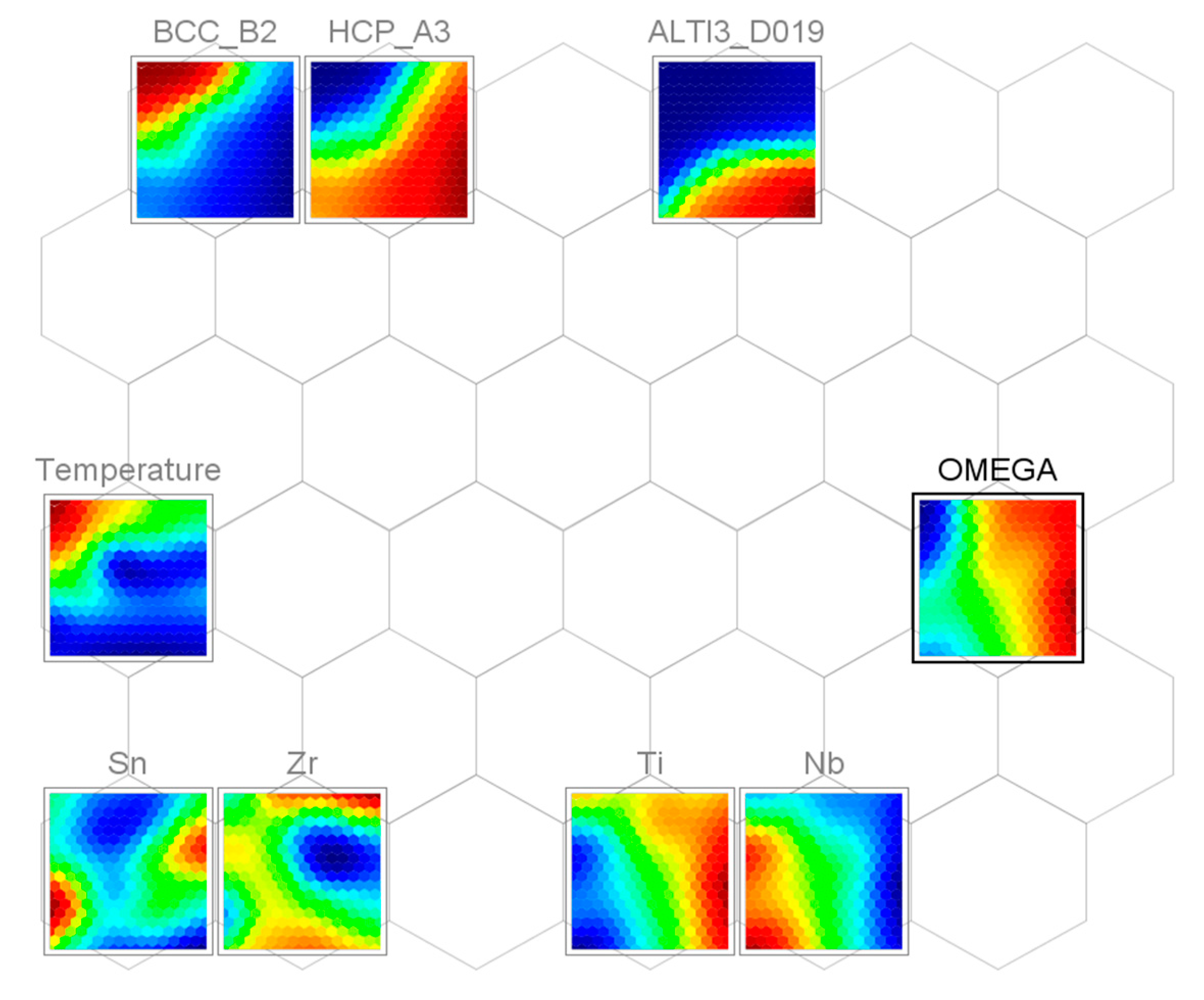
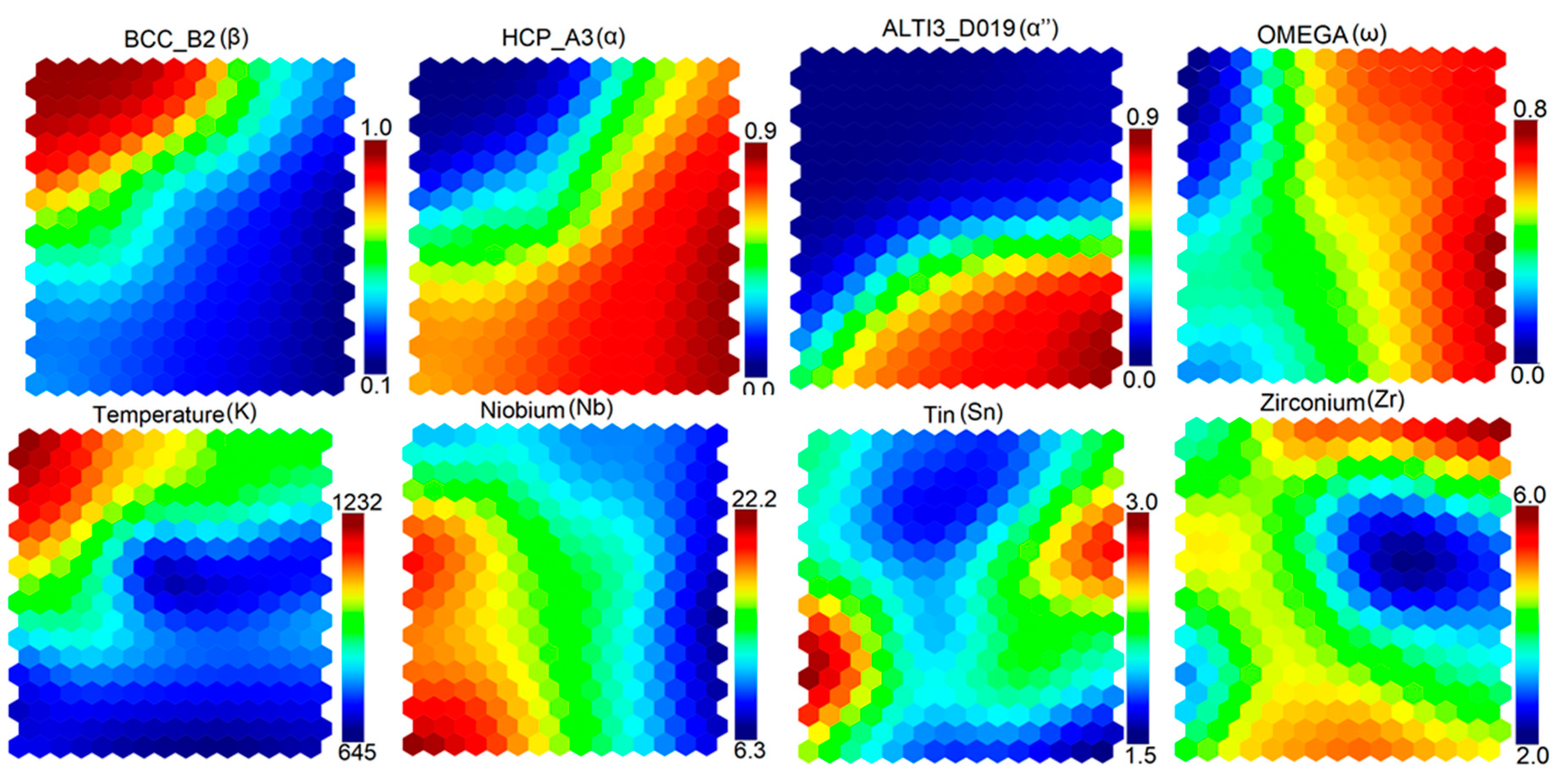
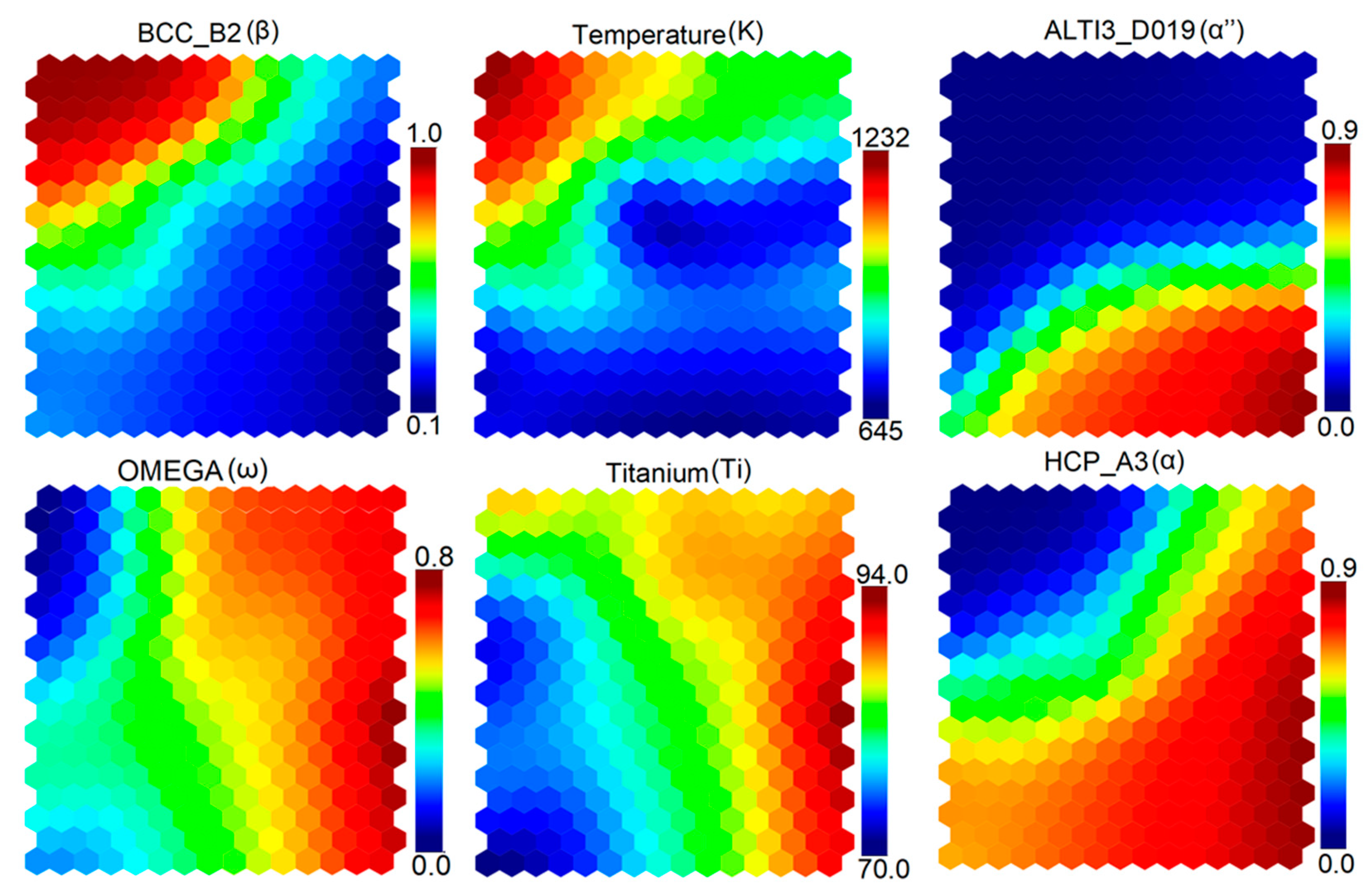
  • The SOM algorithm was used to determine correlations among alloying elements, temperature, and various stable and metastable phases.
  • Finally, we predicted compositions of five select alloys that are expected to meet our expectations regarding the phase stability of β phase.

Author Contributions

Conceptualization, R.J. and G.S.D.; methodology, R.J.; software, R.J.; validation, R.J.; formal analysis, R.J.; investigation, R.J.; resources, R.J. and G.S.D.; data curation, R.J.; writing—original draft preparation, R.J.; writing—review and editing, R.J. and G.S.D.; visualization, R.J.; supervision, G.S.D.; project administration, G.S.D.; funding acquisition, G.S.D. All authors have read and agreed to the published version of the manuscript.

Funding

This work was supported by the College of Engineering and Computing at Florida International University and by NASA HQ University Leadership Initiative (ULI) program under federal award number NNX17AJ96A titled “Adaptive Aerostructures for Revolutionary Supersonic Transportation” managed by Texas A&M University.

Acknowledgments

Authors would like to express their sincere gratitude to Professor Cristian V. Ciobanu from Colorado School of Mines, Golden, Colorado, USA, and Professor Carlo Poloni from ESTECO Co., Trieste, Italy for providing access to some of the commercial software used in this paper. Reviewers’ comments and suggestions helped the readability of this paper and are highly appreciated.

Conflicts of Interest

The authors declare no conflict of interest. The funders had no role in the design of the study; in the collection, analyses, or interpretation of data; in the writing of the manuscript, or in the decision to publish the results.

References

  1. Long, M.; Rack, H. Titanium alloys in total joint replacement—A materials science perspective. Biomaterials 1998, 19, 1621–1639. [Google Scholar] [CrossRef]
  2. Marker, C. Development of a Knowledge Base of Ti-Alloys from First-Principles and Thermodynamic Modeling. Ph.D. Thesis, The Pennsylvania State University, State College, PA, USA, August 2017. Available online: https://www.proquest.com/docview/1988756108 (accessed on 30 October 2019).
  3. Jung, H.D.; Jang, T.S.; Wang, L.; Kim, H.E.; Koh, Y.H.; Song, J. Novel strategy for mechanically tunable and bioactive metal implants. Biomaterials 2015, 37, 49–61. [Google Scholar] [CrossRef] [PubMed]
  4. Lee, H.; Jang, T.S.; Song, J.; Kim, H.E.; Jung, H.D. Multi-scale porous Ti6Al4V scaffolds with enhanced strength and biocompatibility formed via dynamic freeze-casting coupled with micro-arc oxidation. Mater. Lett. 2016, 185, 21–24. [Google Scholar] [CrossRef]
  5. Jang, T.S.; Kim, D.; Han, G.; Yoon, C.B.; Jung, H.D. Powder based additive manufacturing for biomedical application of titanium and its alloys: A review. Biomed. Eng. Lett. 2020, 10, 505–516. [Google Scholar] [CrossRef]
  6. Kolli, R.P.; Devaraj, A. A Review of Metastable Beta Titanium Alloys. Metals 2018, 8, 506. [Google Scholar] [CrossRef] [Green Version]
  7. Mohammed, M.T.; Khan, Z.A.; Siddiquee, A.N. Beta titanium alloys: The lowest elastic modulus for biomedical applications: A review. Int. J. Chem. Nucl. Metall. Mater. Eng. 2014, 8, 726–731. [Google Scholar]
  8. Soundararajan, S.R.; Vishnu, J.; Manivasagam, G.; Muktinutalapati, N.R. Processing of Beta Titanium Alloys for Aerospace and Biomedical Applications. In Titanium Alloys—Novel Aspects of Their Processing; IntechOpen: London, UK, 2018. [Google Scholar]
  9. Magdalen, H.C.; Baghi, A.D.; Ghomashchi, R.; Xiao, W.; Oskouei, R.H. Effect of niobium content on the microstructure and Young’s modulus of Ti-xNb-7Zr alloys for medical implants. J. Mech. Behav. Biomed. 2019, 99, 78–85. [Google Scholar]
  10. Banerjee, S.; Tewari, R.; Dey, G.K. Omega phase transformation—Morphologies and mechanisms. Int. J. Mater. Res. 2006, 97, 963–977. [Google Scholar] [CrossRef]
  11. Mantri, S.; Choudhuri, D.; Behera, A.; Hendrickson, M.; Alam, T.; Banerjee, R. Role of isothermal omega phase precipitation on the mechanical behavior of a Ti-Mo-Al-Nb alloy. Mater. Sci. Eng. A 2019, 767, 138397. [Google Scholar] [CrossRef]
  12. Li, Y.; Yang, C.; Zhao, H.; Qu, S.; Li, X.; Li, Y. New Developments of Ti-Based Alloys for Biomedical Applications. Materials 2014, 7, 1709–1800. [Google Scholar] [CrossRef] [Green Version]
  13. Manivasagam, G.; Singh, A.K.; Asokamani, R.; Gogia, A.K. Ti based biomaterials, the ultimate choice for orthopaedic implants—A review. Prog. Mater. Sci. 2009, 54, 397–425. [Google Scholar] [CrossRef]
  14. Aleixo, G.T.; Afonso, C.; Coelho, A.; Caram, R. Effects of Omega Phase on Elastic Modulus of Ti-Nb Alloys as a Function of Composition and Cooling Rate. Solid State Phenom. 2008, 138, 393–398. [Google Scholar] [CrossRef]
  15. De Fontaine, D.; Paton, N.; Williams, J. The omega phase transformation in titanium alloys as an example of displacement controlled reactions. Acta Met. 1971, 19, 1153–1162. [Google Scholar] [CrossRef]
  16. Ferrari, A.; Paulsen, A.; Langenkämper, D.; Piorunek, D.; Somsen, C.; Frenzel, J.; Rogal, J.; Eggeler, G.; Drautz, R. Discovery of ω-free high-temperature Ti-Ta-X shape memory alloys from first-principles calculations. Phys. Rev. Mater. 2019, 3, 103605. [Google Scholar] [CrossRef] [Green Version]
  17. Ito, A.; Okazaki, Y.; Tateishi, T.; Ito, Y. In vitro biocompatibility, mechanical properties, and corrosion resistance of Ti-Zr-Nb-Ta-Pd and Ti-Sn-Nb-Ta-Pd alloys. J. Biomed. Mater. Res. 1995, 29, 893–899. [Google Scholar] [CrossRef]
  18. Boyce, B.F.; McWilliams, S.; Mocan, M.Z.; Elder, H.Y.; Boyle, I.T.; Junor, B.J.R. Histological and electron microprobe studies of mineralization in aluminum related osteomalacia. J. Clin. Pathol. 1992, 45, 502–508. [Google Scholar] [CrossRef] [Green Version]
  19. Domingo, J.L. Vanadium and Tungsten Derivatives as Antidiabetic Agents. Biol. Trace Elem. Res. 2002, 88, 97–112. [Google Scholar] [CrossRef]
  20. Tane, M.; Akita, S.; Nakano, T.; Hagihara, K.; Umakoshi, Y.; Niinomi, M.; Nakajima, H. Peculiar elastic behavior of Ti–Nb–Ta–Zr single crystals. Acta Mater. 2008, 56, 2856–2863. [Google Scholar] [CrossRef]
  21. Niinomi, M.; Nakai, M.; Hieda, J. Development of new metallic alloys for biomedical applications. Acta Biomater. 2012, 8, 3888–3903. [Google Scholar] [CrossRef]
  22. Aleixo, G.T.; Lopes, E.; Contieri, R.; Cremasco, A.; Afonso, C.R.; Caram, R. Effects of Cooling Rate and Sn Addition on the Microstructure of Ti-Nb-Sn Alloys. Solid State Phenom. 2011, 172, 190–195. [Google Scholar] [CrossRef]
  23. Andersson, J.-O.; Helander, T.; Höglund, L.; Shi, P.; Sundman, B. Thermo-Calc & DICTRA, computational tools for materials science. Calphad 2002, 26, 273–312. [Google Scholar] [CrossRef]
  24. LeCun, Y.; Bengio, Y.; Hinton, G. Deep learning. Nature 2015, 521, 436–444. [Google Scholar] [CrossRef] [PubMed]
  25. Kohonen, T. Self-organized formation of topologically correct feature maps. Biol. Cybern. 1982, 43, 59–69. [Google Scholar] [CrossRef]
  26. TensorFlow. Available online: https://www.tensorflow.org/ (accessed on 30 May 2020).
  27. Keras: The Python Deep Learning Library. Available online: https://keras.io/ (accessed on 30 May 2020).
  28. Jha, R.; Dulikravich, G.S. Design of High Temperature Ti–Al–Cr–V Alloys for Maximum Thermodynamic Stability Using Self-Organizing Maps. Metals 2019, 9, 537. [Google Scholar] [CrossRef] [Green Version]
  29. Jha, R.; Dulikravich, G.S. Solidification and heat treatment simulation for aluminum alloys with scandium addition through CALPHAD approach. Comput. Mater. Sci. 2020, 182, 109749. [Google Scholar] [CrossRef]
  30. Jha, R.; Dulikravich, G.S. Determination of Composition and Temperature Regimes for Stabilizing Precipitation Hardening Phases in Aluminum Alloys with Scandium Addition: Combined CALPHAD—Deep Learning Approach. Calphad 2021. [Google Scholar]
  31. Jha, R.; Dulikravich, G.S.; Chakraborti, N.; Fan, M.; Schwartz, J.; Koch, C.C.; Colaco, M.J.; Poloni, C.; Egorov, I.N. Self-organizing maps for pattern recognition in design of alloys. Mater. Manuf. Process. 2017, 32, 1067–1074. [Google Scholar] [CrossRef]
  32. Jha, R.; Dulikravich, G.S.; Colaco, M.J.; Fan, M.; Schwartz, J.; Koch, C.C. Magnetic Alloys Design Using Multi-Objective Optimization. In Advanced Structured Materials; Oechsner, A., Da Silva, L.M., Altenbac, H., Eds.; Springer: Berlin/Heidelberg, Germany, 2017; Volume 33, pp. 261–284, 978–981. [Google Scholar]
  33. Jha, R.; Chakraborti, N.; Diercks, D.R.; Stebner, A.P.; Ciobanu, C.V. Combined machine learning and CALPHAD approach for discovering processing-structure relationships in soft magnetic alloys. Comput. Mater. Sci. 2018, 150, 202–211. [Google Scholar] [CrossRef] [Green Version]
  34. Jha, R.; Diercks, D.R.; Chakraborti, N.; Stebner, A.P.; Ciobanu, C.V. Interfacial energy of copper clusters in Fe-Si-B-Nb-Cu alloys. Scr. Mater. 2019, 162, 331–334. [Google Scholar] [CrossRef] [Green Version]
  35. Jha, R.; Pettersson, F.; Dulikravich, G.S.; Saxen, H.; Chakraboti, N. Evolutionary Design of Nickel-Based Superalloys Using Data-Driven Genetic Algorithms and Related Strategies. Mater. Manuf. Process. 2015, 30, 488–510. [Google Scholar] [CrossRef]
  36. Thermo-Calc Software: Thermo-Calc Version 2019b. Available online: https://thermocalc.com/release-news/ (accessed on 30 October 2019).
  37. Thermo-Calc Software: TCTI2: TCS Ti/TiAl-Based Alloys Database. Available online: https://thermocalc.com/products/databases/titanium-and-titanium-aluminide-based-alloys/ (accessed on 30 October 2019).
  38. Thermo-Calc Software. Available online: https://thermocalc.com/solutions/solutions-by-material/titanium-and-titanium-aluminide/ (accessed on 30 October 2020).
  39. Thermo-Calc Software TCAL5: TCS Aluminium-Based Alloys Database v.5. Available online: https://www.thermocalc.com/media/56675/TCAL5-1_extended_info.pdf (accessed on 30 August 2019).
  40. Assadiki, A.; Esin, V.A.; Bruno, M.; Martinez, R. Stabilizing effect of alloying elements on metastable phases in cast aluminum alloys by CALPHAD calculations. Comput. Mater. Sci. 2018, 145, 1–7. [Google Scholar] [CrossRef]
  41. TensorBoard: TensorFlow’s Visualization Toolkit. Available online: https://www.tensorflow.org/tensorboard (accessed on 30 May 2020).
  42. ESTECO-ModeFRONTIER. Available online: https://www.esteco.com/technology/analytics-visualization (accessed on 30 May 2020).
  43. Liang, S.; Feng, X.; Yin, L.; Liu, X.Y.; Ma, M.; Liu, R. Development of a new β Ti alloy with low modulus and favorable plasticity for implant material. Mater. Sci. Eng. C 2016, 61, 338–343. [Google Scholar] [CrossRef] [PubMed]
  44. Stefanescu, D.M.; Ruxanda, R. Solidification Structures of Titanium Alloys. In Metallography and Microstructures; ASM International: Geauga, OH, USA, 2004; Volume 9, pp. 116–126. [Google Scholar]
  45. Raabe, D.; Sander, B.; Friák, M.; Ma, D.; Neugebauer, J. Theory-guided bottom-up design of β-titanium alloys as biomaterials based on first principles calculations: Theory and experiments. Acta Mater. 2007, 55, 4475–4487. [Google Scholar] [CrossRef]
  46. Kuroda, P.B.; Quadros, F.D.F.; De Araújo, R.O.; Afonso, C.R.; Grandini, C. Effect of Thermomechanical Treatments on the Phases, Microstructure, Microhardness and Young’s Modulus of Ti-25Ta-Zr Alloys. Materials 2019, 12, 3210. [Google Scholar] [CrossRef] [PubMed] [Green Version]
  47. Sahoo, S.; Chou, K. Phase-field simulation of microstructure evolution of Ti–6Al–4V in electron beam additive manufacturing process. Addit. Manuf. 2016, 9, 14–24. [Google Scholar] [CrossRef]
  48. Ding, L.; Sun, Z.; Liang, Z.; Li, F.; Xu, G.; Chang, H. Investigation on Ti-6Al-4V Microstructure Evolution in Selective Laser Melting. Metals 2019, 9, 1270. [Google Scholar] [CrossRef] [Green Version]
  49. Ahluwalia, R.; Laskowski, R.; Ng, N.; Wong, M.; Quek, S.S.; Wu, D.T. Phase field simulation of α/βmicrostructure in titanium alloy welds. Mater. Res. Express 2020, 7, 046517. [Google Scholar] [CrossRef]
  50. Attar, H.; Ehtemam-Haghighi, S.; Soro, N.; Kent, D.; Dargusch, M.S. Additive manufacturing of low-cost porous titanium-based composites for biomedical applications: Advantages, challenges and opinion for future development. J. Alloys Compd. 2020, 827, 154263. [Google Scholar] [CrossRef]
  51. Trevisan, F.; Calignano, F.; Aversa, A.; Marchese, G.; Lombardi, M.; Biamino, S.; Ugues, D.; Manfredi, D. Additive manufacturing of titanium alloys in the biomedical field: Processes, properties and applications. J. Appl. Biomater. Funct. Mater. 2018, 16, 57–67. [Google Scholar] [CrossRef]
  52. Jakubowicz, J. Special Issue: Ti-Based Biomaterials: Synthesis, Properties and Applications. Materials 2020, 13, 1696. [Google Scholar] [CrossRef] [Green Version]
  53. Majumdar, T.; Eisenstein, N.; Frith, J.E.; Cox, S.; Birbilis, N. Additive Manufacturing of Titanium Alloys for Orthopedic Applications: A Materials Science Viewpoint. Adv. Eng. Mater. 2018, 20, 1800172. [Google Scholar] [CrossRef]
  54. Wei, J.; Sun, H.; Zhang, D.; Gong, L.; Lin, J.; Wen, C. Influence of Heat Treatments on Microstructure and Mechanical Properties of Ti–26Nb Alloy Elaborated In Situ by Laser Additive Manufacturing with Ti and Nb Mixed Powder. Materials 2018, 12, 61. [Google Scholar] [CrossRef] [PubMed] [Green Version]
  55. Imagawa, N.; Inoue, K.; Matsumoto, K.; Ochi, A.; Omori, M.; Yamamoto, K.; Nakajima, Y.; Kato-Kogoe, N.; Nakano, H.; Matsushita, T.; et al. Mechanical, Histological, and Scanning Electron Microscopy Study of the Effect of Mixed-Acid and Heat Treatment on Additive-Manufactured Titanium Plates on Bonding to the Bone Surface. Materials 2020, 13, 5104. [Google Scholar] [CrossRef] [PubMed]
  56. Calignano, F.; Galati, M.; Iuliano, L.; Minetola, P. Design of Additively Manufactured Structures for Biomedical Applications: A Review of the Additive Manufacturing Processes Applied to the Biomedical Sector. J. Health Eng. 2019, 2019, 9748212. [Google Scholar] [CrossRef]
  57. Wang, Z.; Liu, P.; Xiao, Y.; Cui, X.; Hu, Z.; Chen, L. A Data-Driven Approach for Process Optimization of Metallic Additive Manufacturing Under Uncertainty. J. Manuf. Sci. Eng. 2019, 141, 1–51. [Google Scholar] [CrossRef]
  58. Sidambe, A.T. Biocompatibility of Advanced Manufactured Titanium Implants—A Review. Materials 2014, 7, 8168–8188. [Google Scholar] [CrossRef] [Green Version]
  59. Kuroda, K.; Okido, M. Hydroxyapatite Coating of Titanium Implants Using Hydroprocessing and Evaluation of Their Osteoconductivity. Bioinorg. Chem. Appl. 2012, 2012, 1–7. [Google Scholar] [CrossRef] [Green Version]
  60. Lu, R.-J.; Wang, X.; He, H.-X.; Ling-Ling, E.; Li, Y.; Zhang, G.-L.; Li, C.-J.; Ning, C.-Y.; Liu, H. Tantalum-incorporated hydroxyapatite coating on titanium implants: Its mechanical and in vitro osteogenic properties. J. Mater. Sci. Mater. Med. 2019, 30, 111. [Google Scholar] [CrossRef]
  61. Kazimierczak, P.; Przekora, A. Osteoconductive and Osteoinductive Surface Modifications of Biomaterials for Bone Regeneration: A Concise Review. Coatings 2020, 10, 971. [Google Scholar] [CrossRef]
  62. Jaafar, A.; Hecker, C.; Árki, P.; Joseph, Y. Sol-Gel Derived Hydroxyapatite Coatings for Titanium Implants: A Review. Bioengineering 2020, 7, 127. [Google Scholar] [CrossRef]
Figure 1. Occurrence (%) of the OMEGA (ω) phase for different temperature ranges for three separate equilibrium calculations.
Metals 11 00015 g001
Figure 2. SOM components plot for the Ti-Nb-Zr-Sn system.
Metals 11 00015 g002
Figure 3. SOM plot showing chemical concentrations, temperatures and resulting stable and metastable phases for the Ti-Nb-Zr-Sn system.
Metals 11 00015 g003
Figure 4. SOM plot showing composition (Ti), temperature and resulting stable and metastable phases for the Ti-Nb-Zr-Sn system.
Metals 11 00015 g004
Table 1. Concentration bounds for alloying elements (atomic %) for the Ti-Nb-Zr-Sn system and temperature range (K) chosen for study.
NbZrSnTiTemp. (K)
Minimum0.030.020.0158.950.0
Maximum31.69.954.9597.71526.0
Table 2. Performance metrics for deep learning artificial neural network (DLANN) models for various phases for the Ti-Nb-Zr-Sn system.
PhaseDLANN
Architecture
Error Metrics (Validation Set)
Mean Absolute Error (MAE)Mean Squared Error (MSE)
ALTI3_D019(α’’)50-100-100-1000.032860.00549
BCC_B2 (β)80-160-160-1600.031820.00608
BCC_B2#290-180-180-1800.035740.00916
HCP_A3(α)90-180-180-1800.017830.00135
OMEGA (ω)70-140-140-1400.019220.00248
Table 3. Self-organizing maps (SOM) error metrics for the Ti-Nb-Zr-Sn system.
Quantization ErrorTopological Error
0.0640.028
Table 4. Candidate alloys predicted through CALculation of PHAse Diagram (CALPHAD), DLANN models and SOM approach, with zero concentrations of HCP_A3 (α), ALTI3_D019 (α”), and OMEGA (ω) phases.
Alloy No. Ti (Mole %) Nb (Mole %) Zr (Mole %) Sn (Mole %) Temp. (K)
163.1124429.854385.113411.91977641.7
265.5641327.262266.325620.84798807.825
365.4453427.155566.626090.77301955.644
464.1560326.811137.318431.71441989.739
573.2829823.132841.395282.18891024.94
Publisher’s Note: MDPI stays neutral with regard to jurisdictional claims in published maps and institutional affiliations.

