Article

Design, Setup, and Evaluation of a Compensation System for the Light Deflection Effect Occurring When Measuring Wrought-Hot Objects Using Optical Triangulation Methods

Institute for Measurement and Automatic Control, Leibniz University Hannover, Nienburger Strasse 17, 30167 Hannover, Germany
*
Author to whom correspondence should be addressed.
Metals 2020, 10(7), 908; https://doi.org/10.3390/met10070908
Submission received: 10 June 2020 / Revised: 1 July 2020 / Accepted: 3 July 2020 / Published: 7 July 2020
(This article belongs to the Special Issue Hybrid Bulk Metal Components)

Abstract

:
In this paper, we present a system to compensate for the light deflection effect during the optical geometry measurement of a wrought-hot object. The acquired 3D data can be used to analyze the formed geometry of a component directly after a hot forging process without waiting for the needed cooling time to room temperature. This may be used to parameterize the process and to detect defect components early in the production process, among others. The light deflection as the deviation from the linear path of the light is caused by an inhomogeneous refractive index field surrounding the hot object. We present the design and setup for a nozzle-based forced air flow actuator, which suppresses the light deflection effect. The design process includes a simulation of the developing field, as well as of the interaction of the field with an external forced air flow. The cooling effect of the air flow is evaluated, and conclusions are drawn from the conflicting interests of good measurement conditions against the forced cooling of the hot object. The findings are then implemented in the physical setup of the suppression system. The system is evaluated using a previously established method based on optical triangulation and fringe projection. Other occurring effects and their influence on the evaluation are considered and discussed.

1. Introduction

The increasing technical and economical requirements for components have led to mono material bulk metal components reaching the limits of their performance due to the material used. To extend those limits, the use of hybrid components is the subject of current research [1,2]. A high technological potential lays in hybrid bulk metal components that are first joined and then further processed. In the collaborative research center 1153 “Tailored Forming”, such a process chain has been developed [3], following the concept “Put the right material in the right place”. Due to the use of novel material combinations in hot bulk metal forming processes, the development of new evaluation techniques also needs to be considered, e.g., to validate new simulation models [4] for cross-wedge rolling [5]. The distortion induced by the combination of cooling and materials with different thermal expansion coefficients needs to be considered for the analysis of such processes. Therefore, the evaluation of the forming process by analyzing the component after cooling down to room temperature is not sufficient. Instead, the component and especially its geometry need to be measured while in the hot state directly after leaving the forming process. To this end, an optical 3D geometry measurement system based on triangulation can be used [6,7,8]. However, the hot object is surrounded by an inhomogeneous refractive index field, deflecting the measurement light from its linear path [9]. There have been attempts to estimate the effect [10] and methods to compensate its impact on triangulation measurements [11]. However, there are currently no in-line or close-to-line measurement systems that take the light deflection into account or compensate for it. The system presented in this paper aims to close that gap by adding a suppression device for the light deflection effect based on formed and forced air flow to an optical 3D geometry measurement system. The design, setup, and analysis of such a system is described in this paper.

2. Background

In this section, the literature for the methods to estimate the light deflection effect is revisited. The content includes the concept of the background-oriented Schlieren (BOS) method to reconstruct a refractive index field, as well as a presentation of a multi-camera fringe projection system (FPS) to quantify the influence of refractive gradients on triangulation measurements.

2.1. Background-Oriented Schlieren Method

The background-oriented Schlieren method was introduced to estimate density differences in a transparent medium from a set of images [12]. To this end, a contrast-rich and unique background was set up in front of a camera. An image was taken at zero-state as the reference, and additional images were captured during the measurement sequence. The displacement of image points due to the light deflection induced by the density gradient was quantified using suitable algorithms, e.g., Farnbäck et al. [13]. The estimation of the density gradient through the refractive index gradient required extensive knowledge about the measurement setup [14], e.g., the size and position of the refractive index field. This knowledge might be difficult to obtain in changing or unknown measurement conditions.

2.2. Using a Multi-Camera Fringe Projection System to Estimate the Direct Influence of the Light Deflection Effect on Optical Triangulation Measurements

In a previous paper [15], we used redundantly reconstructed 3D points of a multi-camera FPS to estimate the magnitude of the light deflection that was occurring when measuring a red-hot object. There, we concluded that the deviations of redundantly reconstructed points were a valid metric to quantify said effect. The validity of the method was shown using a discrete refractive index influence in the form of a glass plate. While we were not able to use the comparison of single object points, an analysis of all available reconstructed points using a histogram showed resounding results.

3. Proposed Method and Necessary Constraints
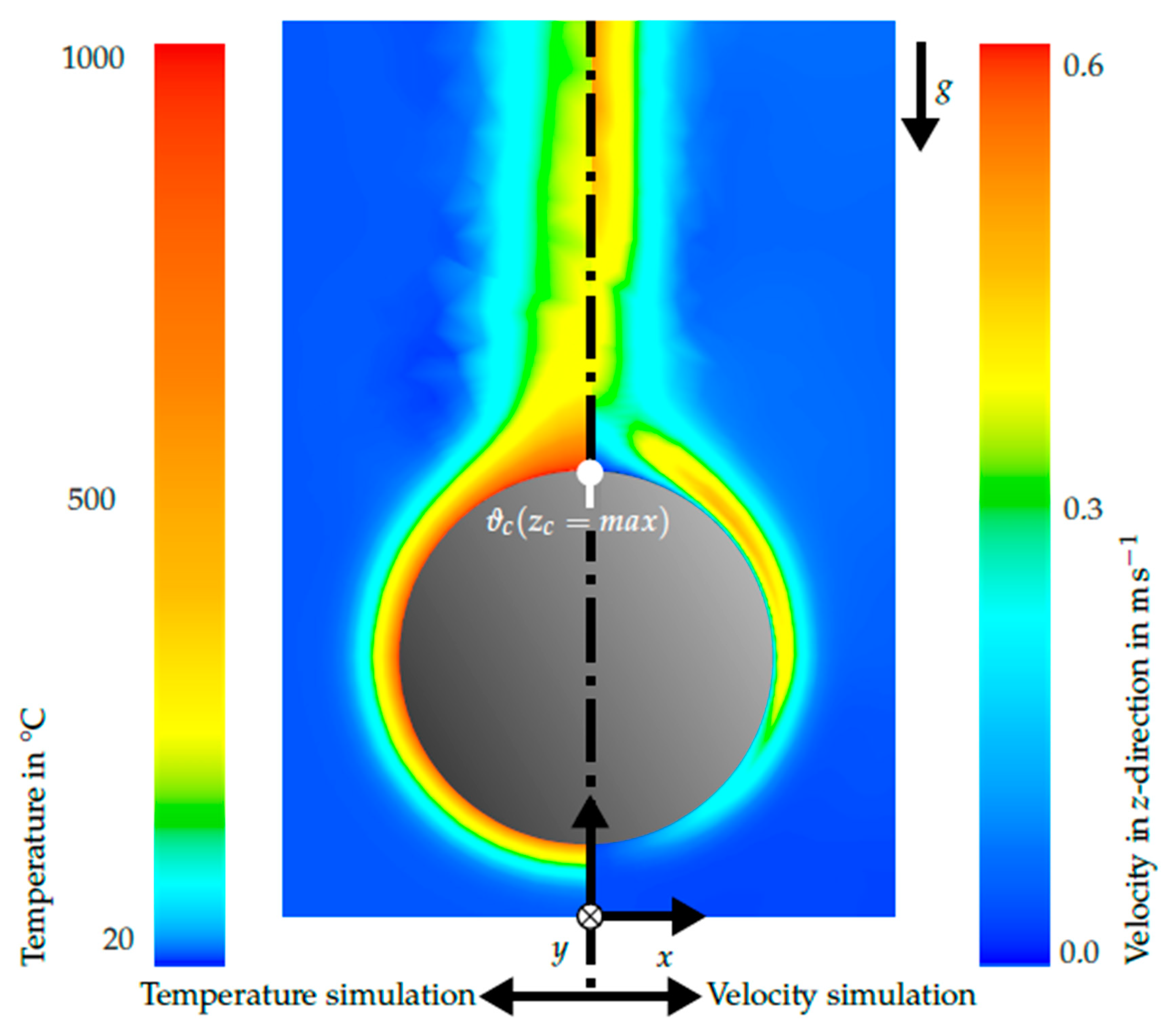
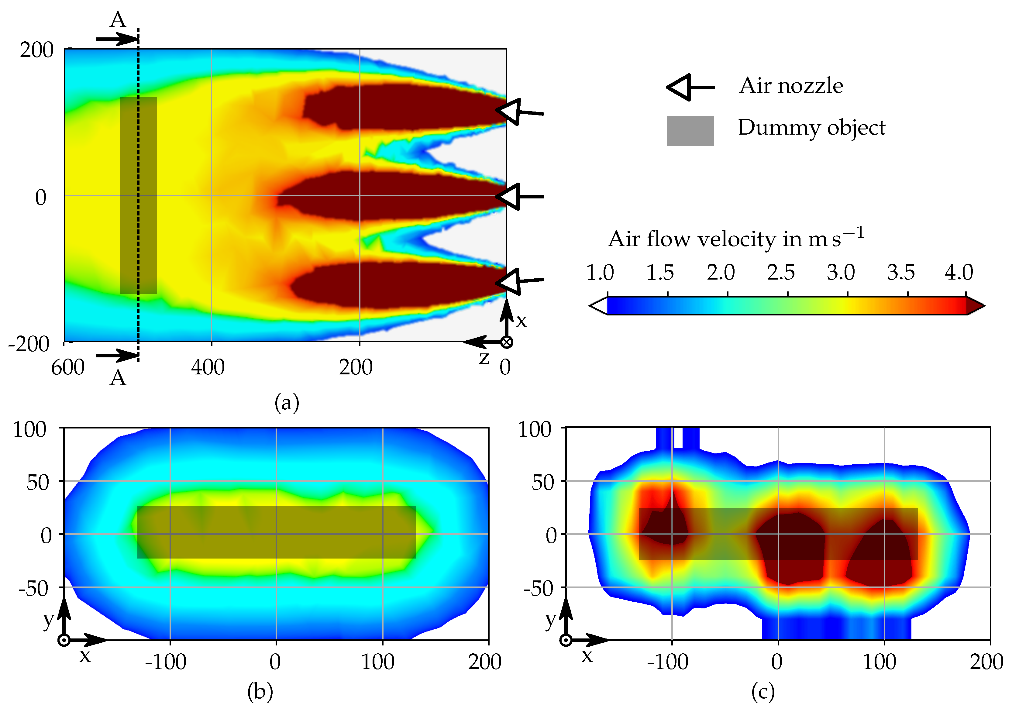
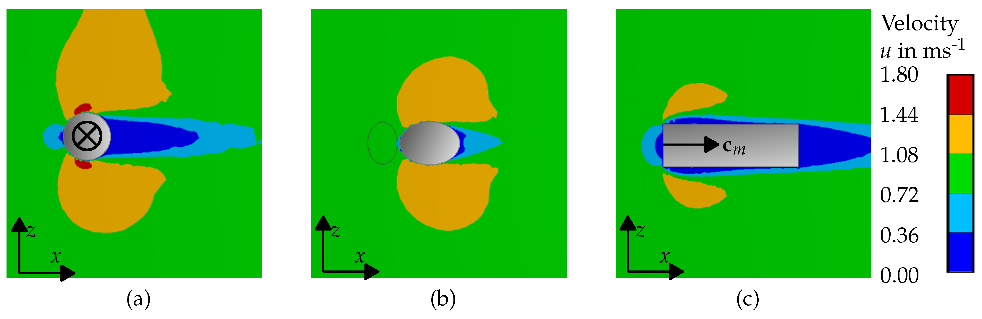
It is proposed to use a forced gas flow in order to reduce the light deflection effect of an inhomogeneous and dynamic refractive index field in an industrial environment. Beermann et al. [9] successfully used a forced laminar gas flow to lower the geometry deviations when measuring a hot rod using a laser light section method. From said article, it was concluded that the forced gas flow needed to be powerful enough to suppress the developed refractive index field while not cooling the hot component too much. To solve this conflicting interest, the velocities and flow parameters were simulated, as well as the cooling effect of such a forced gas flow to a hot component. To this end, the free convection of hot air above a hot cylindrical component needs to be simulated to gain insight into its characteristics. Additionally, the interaction of a forced gas flow with said free convection also needs to be analyzed. The result of that design process yields the necessary construction parameters for the nozzles, as well as the optimal solution for the necessary flow velocities in relation to both the suppression of the refractive index field and the cooling of the component.
The apparatus used for the forming of the forced convection should include an electronically triggered magnetic valve to open and close it conveniently from the same computer that controls the measurement system. To enable operational space for a handling system, as well as for the measurement light, the setup should use nozzle pipes to form the desired air flow at a set distance away from the specimen. The minimum distance was postulated to be approximately 500 m m .

4. Simulation

To design a forced flow apparatus to suppress the light deflection effect successfully, the described conflicting interest between the reduction of the light deflection and the forced cooling of the component needs to be addressed. To this end, the interaction of a forced air flow with the thermal field around an object was simulated to find a compromise. The simulations were conducted using ANSYS Discovery AIM. While the overall aim was to measure the geometry of crank shafts, the simulated object was simplified to a cylinder. Its main axis was concentric to the y-axis of world coordinate system (see Figure 1). It was placed in a rectangular, friction-less flow channel of dimensions d x = 200   m m × d z = 400   m m . The gravitational acceleration of g = 9.81   m   s 1 was assumed to point in negative z-direction. The simulation mode itself was transient and halted after t s = 5   s . At that stage, a stationary state was reached.
To estimate the flow velocities induced by the density gradient around the hot object, the temperature of the cylinder was assumed to be ϑ c = 1000   ° C , while the temperature of the ambient air was set to ϑ = 20   ° C . To simulate a simplified interaction between the nozzle flow and the heat-induced convection, a forced uniform flow was introduced into the simulation. According to Section 3, the direction of the forced flow was in the negative z-direction. The forced flow itself was modeled to be homogeneously distributed in the entire area of the flow channel used. Different forced flow velocities v f f were combined with different cylinder diameters d c to investigate its influence.
The light deflection effect was evaluated in relation to the thickness of air d l with a temperature ϑ a i r > 110   ° C . The thickness of the air layer was extracted from the simulation by measuring in a straight line up from the top center point of the cylinder (see Figure 2b). The cooling of the component was also simulated through the temperature of the topmost point on the cylinder, i.e., ϑ c ( z c = m a x ) .

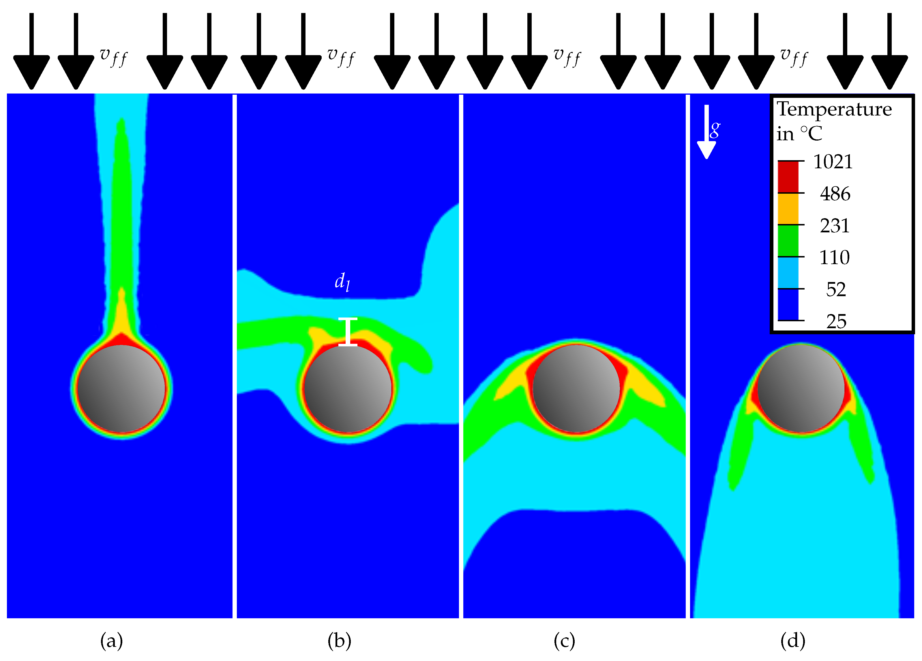
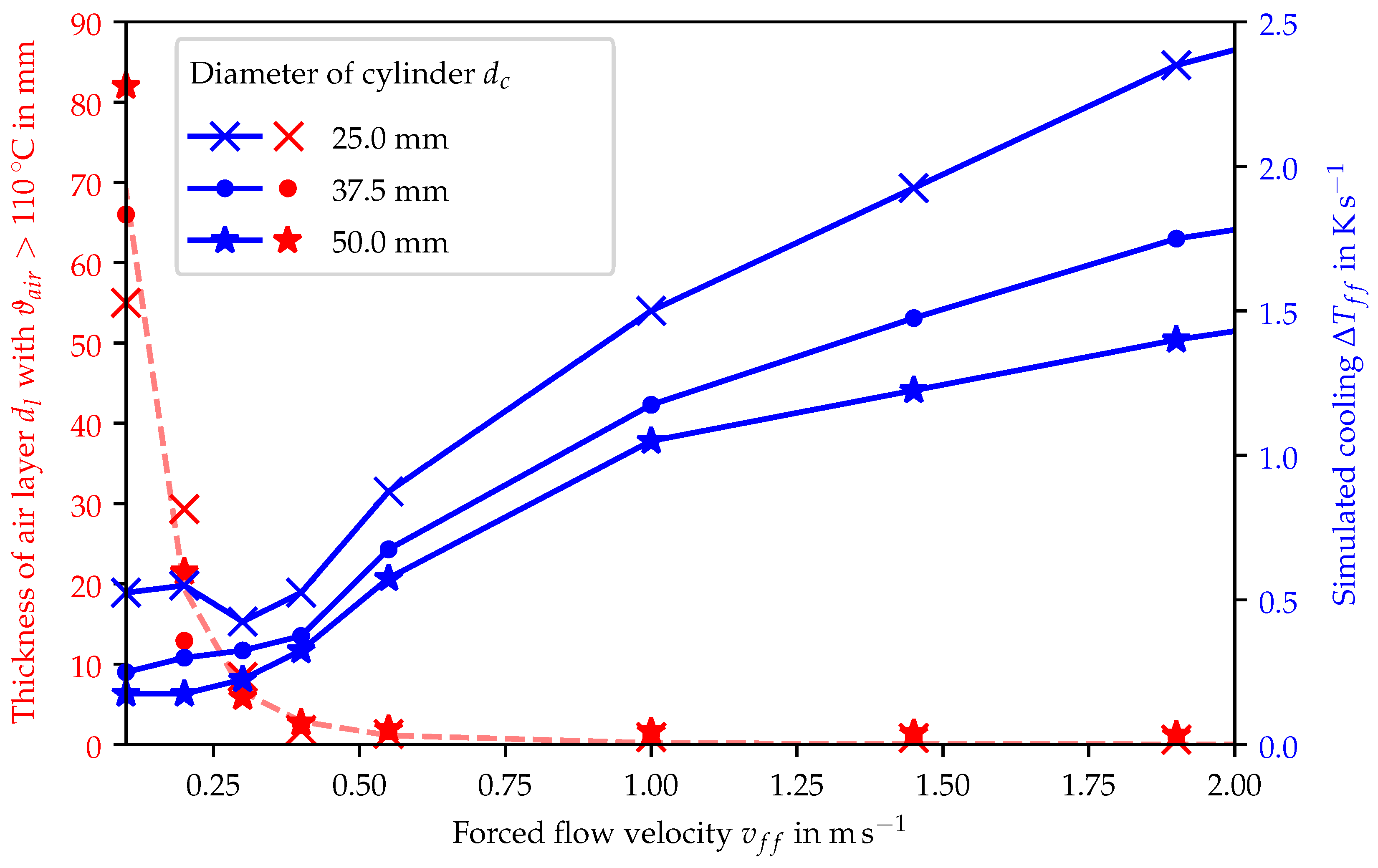
4.1. Simulation Results and Discussion

The developed temperature and velocity fields in the simulation without an additional forced air flow are shown in Figure 1. The size of both fields in y was not investigated here, since only a 2D cylindrical object was simulated. Overall, the shape of the convective flow over the cylindrical object was qualitatively similar to the one measured by, e.g., Beermann [14]. The simulation of the free convection field was therefore considered to be valid.
The effect of different forced air flow velocities on the development of the heat-induced temperature field is shown in Figure 2 in combination with Figure 3. Figure 2 shows the sectional view through the simulated temperature field at different forced flow velocities v f f . There was an equilibrium-like state between v f f and v c f for v f f = 0.2   m   s 1 (see Figure 2b). The simulation results for v f f > 1.0   m   s 1 were conducted (see Figure 2), but are not shown here, since the differences with respect to Figure 2d were considered to be marginal.
Figure 3 shows the relation between the thickness of the air layer d l with ϑ a i r > 110   ° C and the cooling rate Δ T f f as a function of the forced air flow velocity v f f . We estimated a function to fit into the air layer data (red dashed line), corresponding to the general style of:
d l = a b v f f 3 + c .
In this equation, a, b, and c are arbitrary values not corresponding to any physical attributes. The equation itself is similar to an inverse relation between d l and v f f , as the thickness can be considered to be infinite for d l ( v f f 0 ) inf and zero for larger values d l ( v f f inf ) 0 , which corresponded to the development of the field in Figure 2. The displayed line was considered a helpful tool for the visualization of the development of the thickness of the hot air layer; therefore, a description of the optimized parameters was omitted.
Prior to the simulation, the thickness of the air layer was expected to also be a function of the diameter of the cylinder d l = f ( d c ) . This seemed to be the case up to v f f 0.3   m   s 1 , while being less distinct for v f f < 0.3   m   s 1 . The only small differences between the free convection velocities v f c ( d c ) hinted at a marginal influence of the cylinder diameter on the free convection.
Considering the cooling effect of the forced flow onto the cylinder (blue lines in Figure 3), the results showed an increasing cooling effect with increasing flow velocities. The cooling effect was assumed to be inversely proportional to the radius of the cylinder, which was considered to be due to the decreasing volume-surface quotient.

4.2. Simulation Conclusions
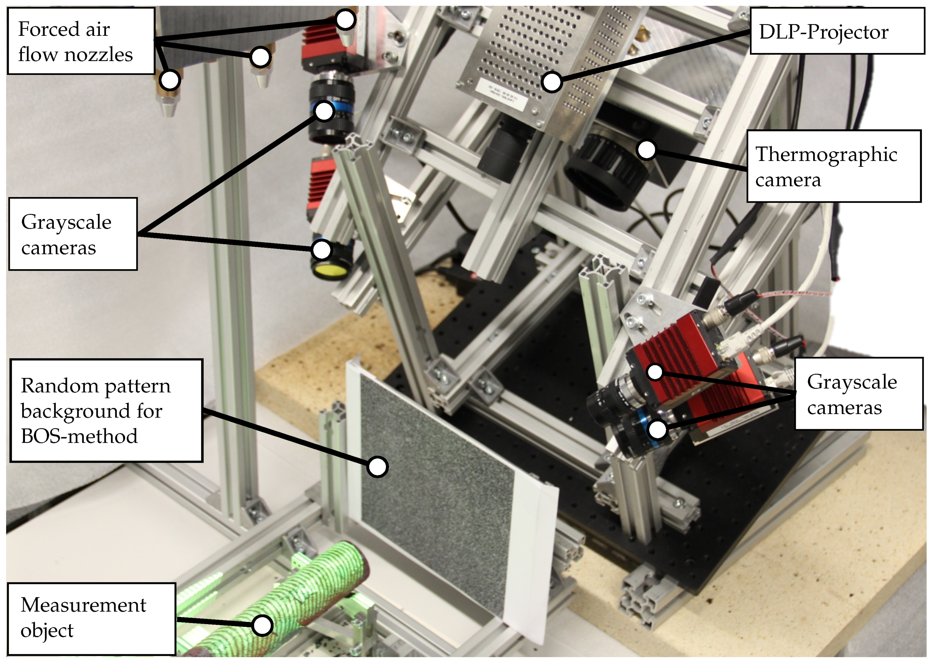
The simulations showed a direct connection between forced flow velocity v f f to the layer thickness d l and the cooling rate Δ T f f . While a minimum layer thickness was desired, the reduction of the layer thickness for flow velocities v f f > 1   m   s 1 was considered marginal compared to the increase of the cooling rate Δ T f f through the forced air flow. Therefore, the flow velocities for the design of the actuator were chosen to be 1   m   s 1 < v f f < 4   m   s 1 across the whole cylinder surface, assuming a linear increase in cooling Δ T f f with further increasing v f f .
To transfer the findings from the simulation to the design of a laboratory setup, a setup with three nozzles was implemented. The main aim was to achieve a mostly homogeneous velocity distribution over the area of a cylinder (diameter d c = 50   m m ; length l c = 250   m m ) at a distance of 500 m m . The comparison between the simulated velocities and the measured velocities of the nozzle setup is shown in the following Section 5. When considering the interaction between the light from the FPS and the forced air flow, it was concluded that the measurement light would most be affected by the warmer areas under the hot object (light blue areas in Figure 2c,d). Therefore, the combined setup should include nozzles and FPS viewing the object from roughly the same direction.

5. Setup

The setup for the experiments is presented in this section. An image of the complete setup is shown in Figure 4. The measurement system followed the concept of multi-camera fringe projection profilometry and was based on the findings of Bräuer-Burchard et al. [16] and Reich et al. [17]. We explained the calibration and the main functions of the measurement system in a previous paper [15]. The forced air flow actuator consisted of three commercially available nozzles with a minimum inner diameter of d n = 0.8   m m and a custom-made aluminum connection block. The design study examining different flow directions and nozzle setups resulting in the presented setup is shown in Appendix A. The connection block placed the nozzles at equidistant points on a line with 100 m m in between them and an angle to the outside of 5 ° . A magnetic valve and a manually operated pressure regulator connected the nozzles to the pressurized air container in the laboratory. An image of the nozzles is part of Figure 4 (upper left). The nozzles were set up above the measurement object to use the occurring forces to hold the measurement object in place. To ensure that the measurement light and the forced air flow took similar paths, the FPS was also mounted above the object. Depending on the air pressure p f f set in the pressure regulator, the velocities of the air flow field were controlled. Figure 5 shows the designed and simulated velocity field in comparison to a measured field using an air pressure of p f f = 2.5   bar . The flow velocity measurements were conducted using a scale and a hand-held anemometer. The flow velocity field showed significant differences from the simulated velocity field in magnitude and in form. The main reasons for the different shapes lied in the lack of a concentric effect of screw threads, which were used to connect the nozzles and the connection block. The differences in velocity magnitude were mainly due to the low accuracy of the hand-held anemometer, as well as numerical dispersion and diffusion effects in the simulation.
Even though there were velocity differences of up to 90, the overall design process was considered successful, since the aim of surrounding a cylinder ( d c = 50   m m ,   l c = 250   m m ) with an homogeneous air flow field with 1 m / s < v f f < 4 m / s was achieved.

6. Experiments

For the experiments, the magnetic valve for the forced air flow was connected to the projecting sequence of the measurement system using a software trigger. To ensure a fully developed air flow field and account for triggering delays, the projection of the first image was delayed by t d , 0 = 0.3   s compared to the opening of the magnetic valve. The measurement sequence started with a measurement without the air flow and was followed by a measurement with an active flow system to reduce the effect of cooling on the analysis and ensure a fully developed refractive index field during the measurement without forced air flow.

6.1. Experimental Plan

To evaluate the influence of the forced air flow on the light deflection effect, different experiments were conducted:
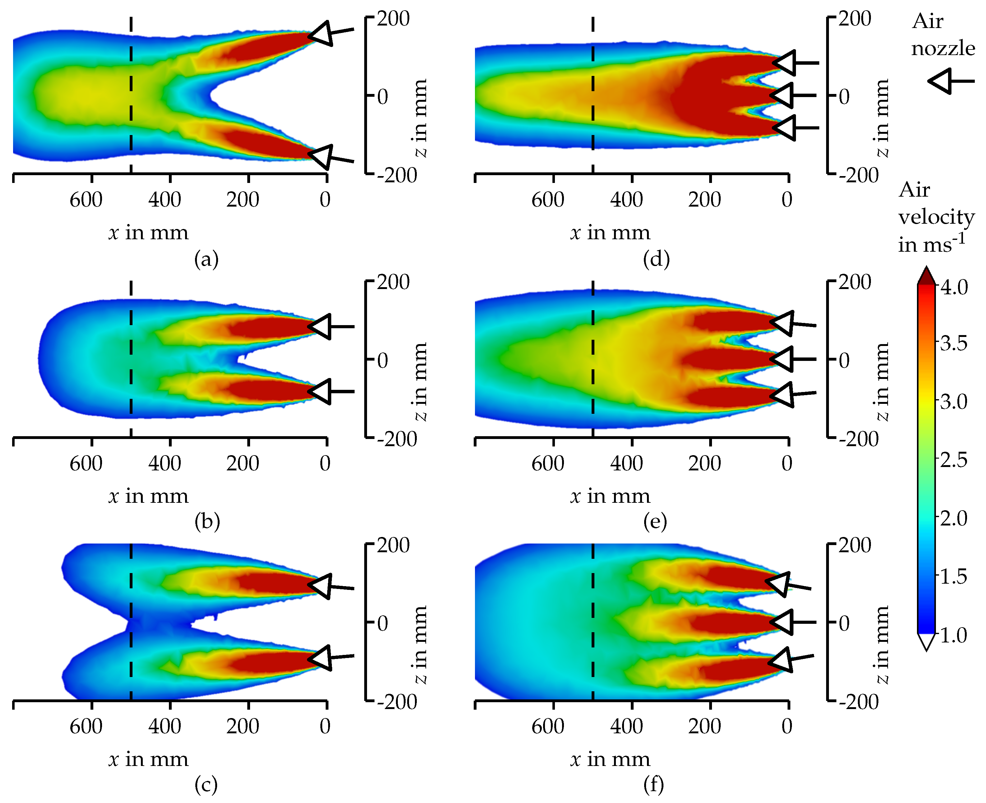
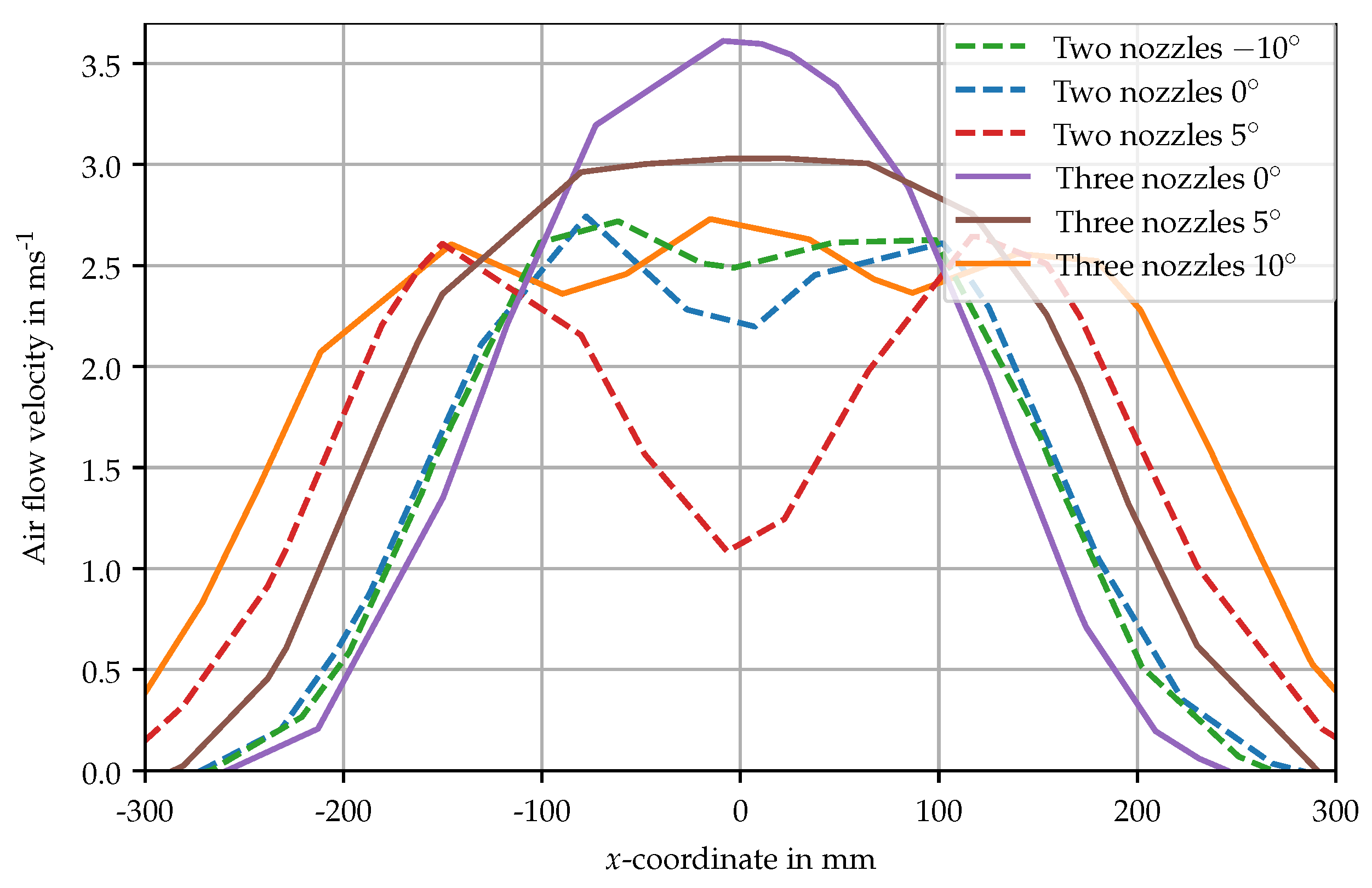
  • Measurement of the cooling effect of the forced air flow onto the cylinder,
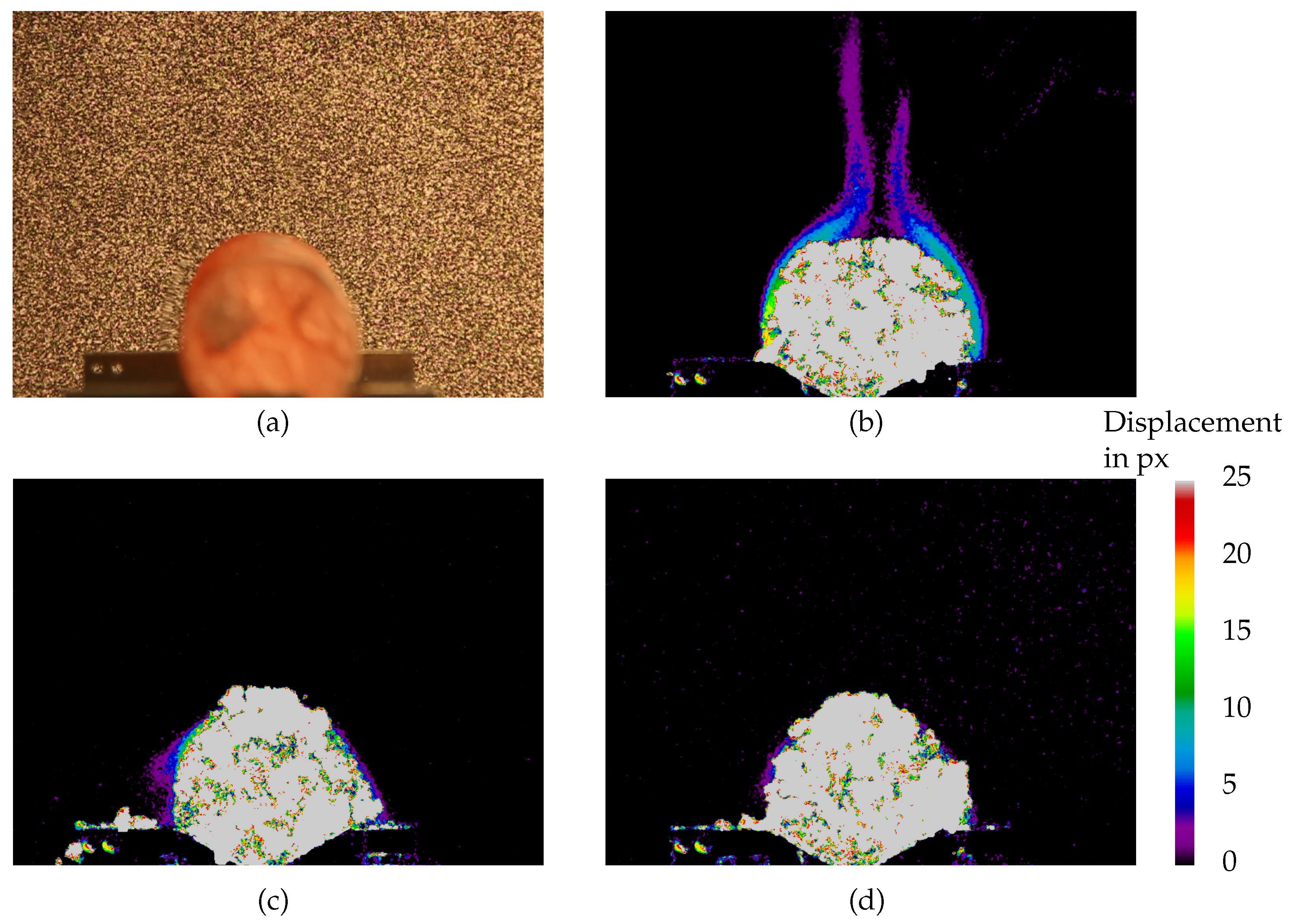
  • using the pixel displacement from the BOS method to estimate the indirect influence of the air flow on the light deflection effect and
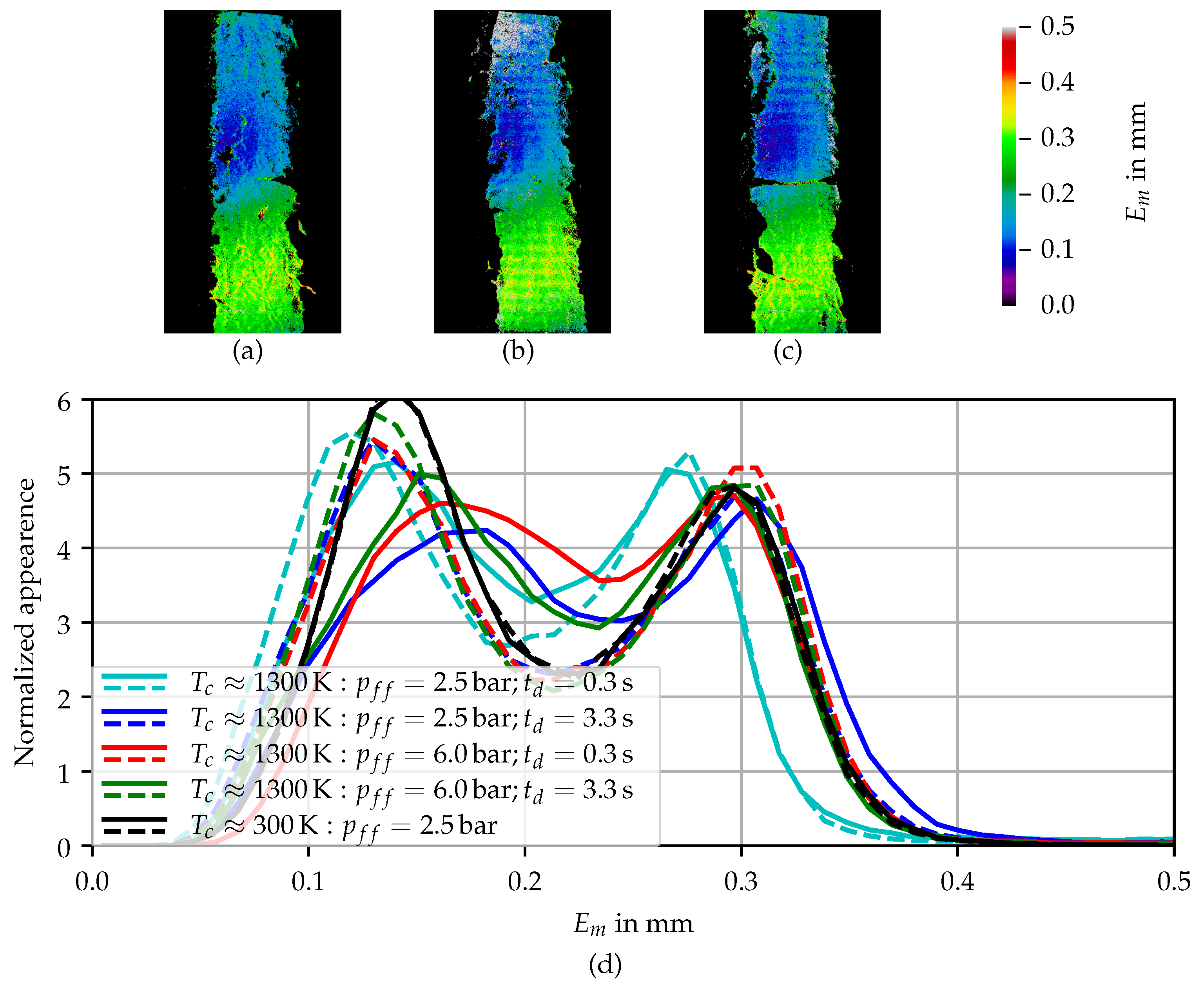
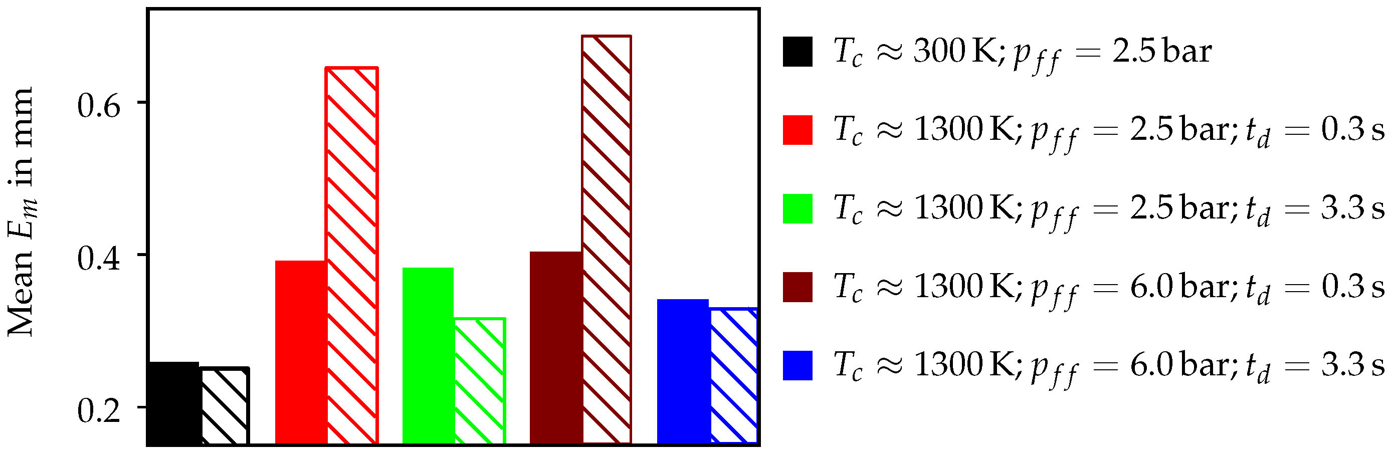
  • analysis of the direct influence by means of using the reconstruction error metric.
The cooling effect (1) was measured using the thermographic infrared (IR) camera (VarioCAM from InfraTec, Dresden, Germany, with a maximum frame rate of 10 Hz ) mounted underneath the projector (see Figure 4). To this end, a red-hot cylinder was measured for a duration of 18 s at the maximum frame rate. During the temperature measurement, the magnetic valve was opened for 8 s . The emission coefficient was set to one ( ε = 1 ) , and the mean temperature of an arbitrarily selected rectangle is plotted in relation to the passed time in Figure 6.
To estimate the size of a refractive gradient field qualitatively (2), the BOS method was used. To this end, a video camera (not shown) was placed in front of the random pattern background without the measurement object in between both. The video capture was started before the hot cylinder was placed. After an undisclosed time delay, the magnetic valve was opened. The first image of the video was used as the reference image to calculate the results. Here, the pixel displacement was used as a means to quantify the light deflection relatively, since a reconstruction of valid refractive index values required extensive a priori knowledge about the setup and the measured field. This procedure was valid in the presented case, since the experiments were conducted without moving any parts of the setup during the video sequence.
To analyze the effect of the interaction of the forced air flow actuator and refractive index field on triangulation measurements (3), the multi-camera FPS was used. Here, the cylinder was placed, and a reference measurement without active air flow was conducted. This was directly succeeded by activating the air flow actuator, waiting a defined delay time t d , and then, triggering the start of the measurement. This procedure reduced the uncertainties induced by moving or exchanging the objects, as discussed in [15]. There was a difference between the direct and the indirect method of estimation for the light deflection effect. This was mainly due to the different paths of light that were examined. When evaluating Figure 4, it is clear that the light for the FPS was traversing different paths compared to the view rays for the BOS method. Due to the 2D nature of the BOS measurement setup, the pixel-wise magnitude of the light deflection effect could not be correlated directly to the reconstructed 3D points. Additionally, the random pattern background used for BOS measurements was blocking the field of view of the lower cameras and of the IR camera. Therefore, the experiments were not carried out simultaneously.

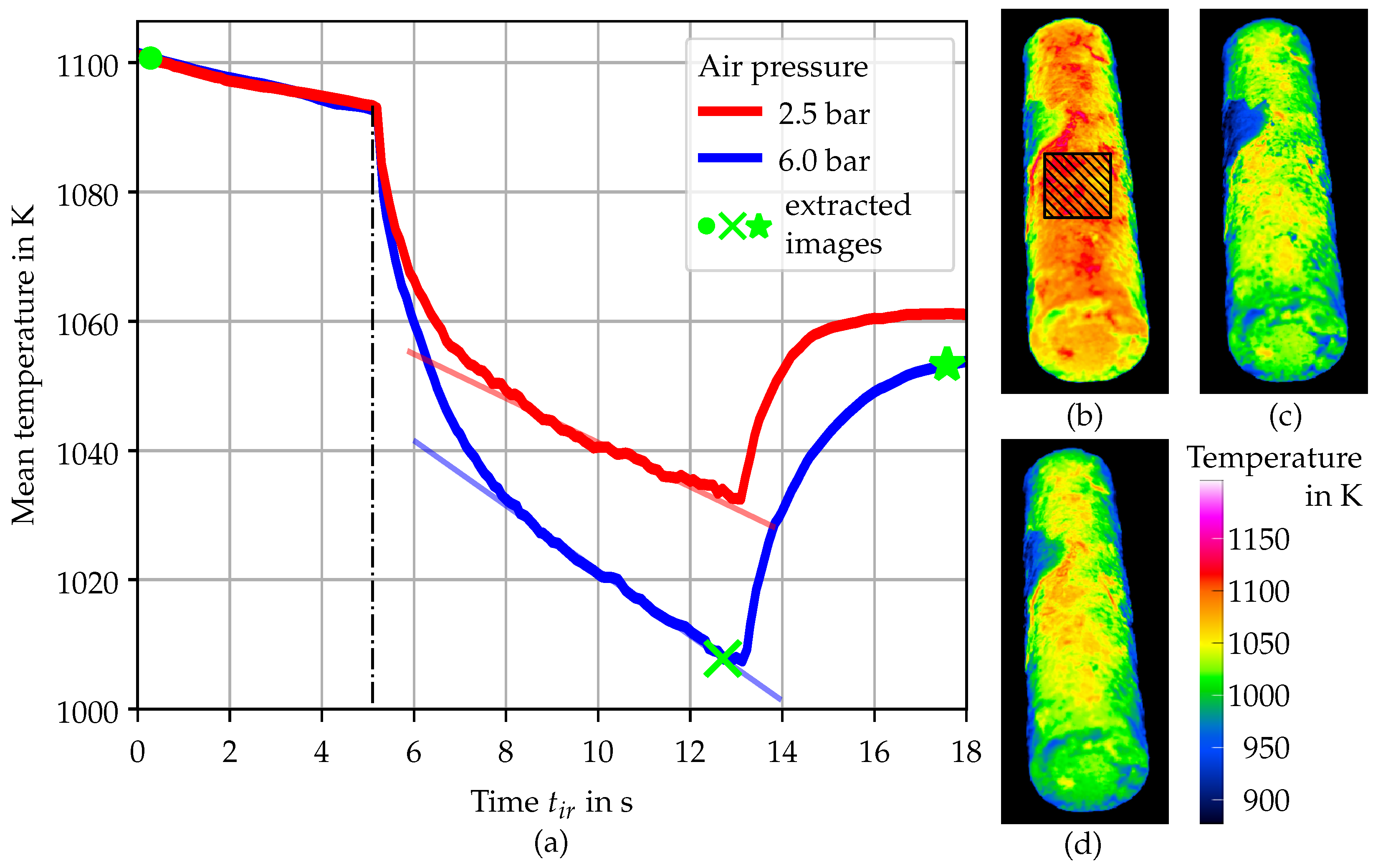
6.2. Experimental Results

The results from the cooling analysis are shown in Figure 6. The thermographic images (Figure 6b–d) are excerpts from the full sequence of images at specific points in time (see the green spots in Figure 6a). To estimate the cooling rate Δ T f f , linear functions were fitted into the sectors with constant gradients. The slope of these functions was the cooling rate and summarized in Table 2.
The results from the BOS experiment are shown in Figure 7. The high displacement values in Figure 7b–d in the lower middle were a result of the hot cylinder not being in place when the reference image was shot. Therefore, the distance from a similar looking pixel group in the reference image was high.
The estimated influence of the refractive index field was observable in the comparison of the measurement of the cold object and the object in the red-hot state (see Figure 8) using the direct estimation method and the multi-camera FPS. The mean values of the shown histograms are found in Table 3 and Figure 9. The reconstruction error E m in the reconstruction quality maps (Figure 8a–c) was not homogeneously distributed, with higher E m values in the upper parts of the images, corresponding to points further away from the FPS. Both the reconstruction quality maps and the histograms showed only marginal differences between the experiments. An example of the reconstructed 3D datasets is shown in Appendix B.
Other observations during the experiment included a noticeable cooling of the component during the measurement as observable through a change of color. The applied force of the air field did not cause any visible vibration or movement of the object.

7. Discussion

Overall, the direct effect of the forced air flow on the development of a refractive index field around a hot cylinder was shown using the BOS method. The qualitative influence was similar in the simulation and measurement (compare Figure 5 and Figure 7).
However, the effect was less distinguishable in the FPS measurements (see Figure 8 and Table 3). Here, the activation of the air flow yielded higher reconstruction errors for the immediate use ( t d = 0.3   s ) of the forced air flow compared to the uninfluenced measurement (compare the dashed and solid red and cyan lines in Figure 8d). This indicated a contradiction: the size of the light-deflecting refractive index field was reduced, but the reconstruction error was increased. In the presented setup, the change of the radiation color of the specimen might have an increasing influence on the reconstruction quality. A cooling of the object resulting in a lowering of the radiation through self-emission was observed during the experiment and could be concluded from the thermographic measurement (see Figure 6). To investigate the stated matter, the necessary time delay between the activation of the air flow and the start of the projection sequence was estimated to be between the start of the flow activation (dotted-dashed line) and the start of the linear temperature development at t i r 8.0   s . Adding the activation time t d , 0 resulted in an improved time delay of t d = 3.3   s . The result of the implementation of this improved delay is shown in Figure 8 (blue/green lines). It is obvious that the improved time delay resulted in an improvement in the estimated reconstruction quality compared to the initial time delay t d = t d , 0 = 0.3   s , as well as the measurement without the forced air flow.
Any concerns about an induced vibration through the forced air flow and a resulting decrease of reconstruction quality could be dispelled through the comparison of the measurements at T c 300   K . If any vibration would have been induced, a significant increase in the reconstruction error metric would have been noticed.

8. Conclusions

Overall, the influence of the forced air flow on the light deflection effect was shown. The BOS measurement showed a significant reduction in pixel displacement, which was considered to be proportional to the light deflection. However, the results from the reconstruction quality experiment showed an only marginal improvement through the forced air flow. The reasons for this were already stated in the previous section and seemed plausible considering the results from the cooling experiment and the improved time delay. However, the reconstruction quality for this setting was lower compared to the experiment at T c 300   K . Therefore, the change of radiation color through cooling needs to be investigated as an additional influence on the optical geometry measurement of hot objects.
This indicated a superposition of effects: on the one hand, the reduced light deflection resulted in a reduced reconstruction error metric while there needed to be an additional effect to then increase the error metric again. The underlying effect here might be the change of the surface color during the air flow induced cooling. The fringe projection reconstruction technique based on Peng’s multi-frequency phase-shift method [18] used requires a constant ambient illumination strength. This ambient light influence is compensated using the temporal average of the phase shift sequence of the highest frequency. A change of background illumination may cause an error in phase reconstruction for each camera and, therefore, a change in the reconstruction error metric. However, a further investigation of this matter is beyond the scope of this paper and is therefore omitted.

9. Summary and Future Work

In this paper, a setup was presented to reduce the light deflection effect when using optical triangulation systems to measure the geometry of a red-hot object. A simulation was used to estimate the velocity of the free convection around the hot object. The same tool simulated the interaction of a forced convection flow with the free convection to gain insight into the necessary flow velocities to suppress the development of the refractive index field around the hot object. That knowledge was used to simulate and implement a forced air flow actuator to be used in combination with a fringe projection system. The effect of this actuator on the light deflection effect was indirectly estimated using a BOS-based method and directly measured using a reconstruction error metric. While the indirect method showed a minimization of the refractive index field, the direct method showed a reduction of the reconstruction error while not reaching the quality level of the measurement of a cold object. Different reasons for this behavior were discussed, but not further investigated.
Overall, the aim of the developed setup (reduction of reconstruction error) was reached while not being sufficient in comparison with a standard measurement. While the design method resulted in a successful development of the setup, it may not be generalizable due to changing boundary conditions when varying the geometry of the measurement object. The developed setup in the present configuration may be used to inspect shaft-like components.
In the future, an investigation of the changing surface color due to the cooling effect of the forced air flow needs to be conducted. Findings of this investigation can then be used to compensate for a changing background color, if the effect is found to be significant.

Author Contributions

Conceptualization, L.Q., C.R. and R.B.; Data curation, L.Q. and C.R.; Formal analysis, L.Q. and R.B.; Funding acquisition, M.K. and E.R.; Investigation, L.Q. and C.R.; Methodology, L.Q.; Project administration, M.K. and E.R.; Resources, L.Q.; Software, L.Q.; Supervision, M.K. and E.R.; Validation, L.Q.; Visualization, L.Q. and C.R.; Writing—original draft, L.Q.; Writing—review & editing, C.R. and M.K. All authors have read and agreed to the published version of the manuscript.

Funding

This research was funded by Deutsche Forschungsgemeinschaft (DFG); Collaborative Research Centre 1153 (CRC) Process Chain to Produce Hybrid High-performance Components Through Tailored Forming (252662854); Subproject C5 Multiscale Geometry Inspection of Joining Zones.

Conflicts of Interest

The authors declare no conflict of interest.

Abbreviations

The following abbreviations are used in this manuscript:
BOSBackground-oriented Schlieren
FPSFringe projection system
IRInfrared

Appendix A. Simulated Case Study

The results from the simulated case study are shown in Figure A1 regarding the direction of the forced air flow and in Figure A2 for the design of the nozzle setup. Analyzing the direction of the air flow focuses on areas that exhibit low air flow velocities ( u < 0.36   m   s 1 ) . The air stays in the same place in these areas and is consequently heated by the hot cylinder. Therefore, there will be a refractive index gradient in these areas at a magnitude comparable to the gradient without air flow. For the given reasons, the air flow should be applied comparable to Case (a), i.e., perpendicular to the cylinder main axis. In all cases, the measurement system should be placed near the forced air flow actuator to avoid areas of low air flow velocities interfering with the measurement light.
Focusing on the nozzle setup, a case study was conducted using ANSYS Discovery AIM. The examined cases are shown in Figure A2. The results are comparable to the ones in Figure 5 while showing a slightly different excerpt from the simulation field. Analyzing the case study, an homogeneous velocity profile of 250 m m at a distance of 500 m m to the nozzles (cf. dashed lines in Figure A2) is considered to be desirable (cf. Section 5). A sectional view through the simulated velocities fields is shown in Figure A3. The simulated profiles are symmetrical to x = 0   m m . The setup using three nozzles and an angle of 5 ° show a nearly homogeneous profile at approximately 3.0 m   s 1 for 125   m m < x < 125   m m . This is the chosen nozzle configuration for the suppression device.
Figure A1. Results from the simulated case study examining different forced air flow v f f = 1.0   m   s 1 directions in relation to a cylinder. The direction is varied by tilting the object and is described by the cylinder main axis c m in world coordinates. The vector for the direction of the forced air flow is ( 1 , 0 , 0 ) T . (a) c m = ( 0 , 1 , 0 ) T ; (b) c m = ( 1 , 1 , 0 ) T ; (c) c m = ( 1 , 0 , 0 ) T .
Metals 10 00908 g0a1
Figure A2. Results from the simulated case study using multiple nozzles. A positive angle value indicates nozzles pointing towards each other, and a negative value indicates nozzles pointing away from each other. The dashed line depicts the design distance, in which an homogeneous field is desired. Air flow velocities v f f < 1.0   m   s 1 are masked and depicted in white. (a) Two nozzles 400 mm apart with an angle of 10 ° ; (b) two nozzles 200 mm apart with an angle of 0 ° ; (c) two nozzles 200 mm apart with an angle of 5 ° ; (d) three nozzles with an angle of 0 ° ; (e) three nozzles with an angle of 5 ° ; (f) three nozzles with an angle of 10 ° .
Metals 10 00908 g0a2
Figure A3. Sectional view through the air flow velocities profiles of Figure A2 (dashed lines).
Metals 10 00908 g0a3

Appendix B. 3D Geometry Reconstructions

An example set of reconstructed height maps z ( u p ) is shown in Figure A4. These height maps are the fundamentals to calculate the deviations maps E m ( u p ) . There is one height map for each camera-camera and camera-projector pair. The height maps reconstructed from cameras on the same side of the measurement setup are omitted (explained in detail in [15]).
Figure A4. Example of a set of reconstructed height maps, depicted as the map of the corresponding z-values. (ah) Height maps from each camera-camera pair and each camera-projector pair, respectively; (i) average height map of all available sets. All points are masked that are not present in each height map. Masked points are not considered when calculating the reconstruction quality metric.
Metals 10 00908 g0a4

References

  1. Behrens, B.A.; Chugreev, A.; Selinski, M.; Matthias, T. Joining zone shape optimisation for hybrid components made of aluminium-steel by geometrically adapted joining surfaces in the friction welding process. AIP Conf. Proc. 2019, 2113, 040027. [Google Scholar]
  2. Behrens, B.A.; Chugreev, A.; Matthias, T.; Poll, G.; Pape, F.; Coors, T.; Hassel, T.; Maier, H.J.; Mildebrath, M. Manufacturing and evaluation of multi-material axial-bearing washers by tailored forming. Metals 2019, 9, 232. [Google Scholar] [CrossRef] [Green Version]
  3. Uhe, J.; Behrens, B.A. Manufacturing of Hybrid Solid Components by Tailored Forming. In Production at the Leading Edge of Technology; Springer: Berlin/Heidelberg, Germany, 2019; pp. 199–208. [Google Scholar]
  4. Böhm, C.; Kruse, J.; Stonis, M.; Aldakheel, F.; Wriggers, P. Virtual Element Method for Cross-Wedge Rolling during Tailored Forming Processes. Procedia Manuf. 2020, 47, 713–718. [Google Scholar] [CrossRef]
  5. Kruse, J.; Jagodzinski, A.; Langner, J.; Stonis, M.; Behrens, B.A. Investigation of the joining zone displacement of cross-wedge rolled serially arranged hybrid parts. Int. J. Mater. Form. 2019, 1–13. [Google Scholar] [CrossRef]
  6. Hawryluk, M.; Ziemba, J.; Sadowski, P. A review of current and new measurement techniques used in hot die forging processes. Meas. Control 2017, 50, 74–86. [Google Scholar] [CrossRef]
  7. Han, L.; Cheng, X.; Li, Z.; Zhong, K.; Shi, Y.; Jiang, H. A Robot-Driven 3D Shape Measurement System for Automatic Quality Inspection of Thermal Objects on a Forging Production Line. Sensors 2018, 18, 4368. [Google Scholar] [CrossRef] [Green Version]
  8. Mejia-Parra, D.; Sánchez, J.R.; Ruiz-Salguero, O.; Alonso, M.; Izaguirre, A.; Gil, E.; Palomar, J.; Posada, J. In-Line Dimensional Inspection of Warm-Die Forged Revolution Workpieces Using 3D Mesh Reconstruction. Appl. Sci. 2019, 9, 1069. [Google Scholar] [CrossRef] [Green Version]
  9. Beermann, R.; Quentin, L.; Pösch, A.; Reithmeier, E.; Kästner, M. Light section measurement to quantify the accuracy loss induced by laser light deflection in an inhomogeneous refractive index field. In Proceedings of the SPIE Optical Metrology, Optical Measurement Systems for Industrial Inspection X, Munich, Germany, 25–29 June 2017; Volume 10329, p. 103292T. [Google Scholar]
  10. Quentin, L.; Beermann, R.; Pösch, A.; Reithmeier, E.; Kästner, M. 3D geometry measurement of hot cylindric specimen using structured light. In Proceedings of the SPIE Optical Metrology, Optical Measurement Systems for Industrial Inspection X, Munich, Germany, 25–29 June 2017; Volume 10329, p. 103290U. [Google Scholar]
  11. Beermann, R.; Quentin, L.; Reithmeier, E.; Kästner, M. Fringe projection system for high-temperature workpieces–design, calibration, and measurement. Appl. Opt. 2018, 57, 4075–4089. [Google Scholar] [CrossRef] [PubMed]
  12. Richard, H.; Raffel, M. Principle and applications of the background oriented schlieren (BOS) method. Meas. Sci. Technol. 2001, 12, 1576. [Google Scholar] [CrossRef]
  13. Farnebäck, G. Two-frame motion estimation based on polynomial expansion. In Scandinavian Conference on Image Analysis; Springer: Berlin/Heidelberg, Germany, 2003; pp. 363–370. [Google Scholar]
  14. Beermann, R.; Quentin, L.; Pösch, A.; Reithmeier, E.; Kästner, M. Background oriented schlieren measurement of the refractive index field of air induced by a hot, cylindrical measurement object. Appl. Opt. 2017, 56, 4168–4179. [Google Scholar] [CrossRef] [PubMed]
  15. Quentin, L.; Beermann, R.; Kästner, M.; Reithmeier, E. Development of a reconstruction quality metric for optical three-dimensional measurement systems in use for hot-state measurement object. Opt. Eng. 2020, 59, 064103. [Google Scholar] [CrossRef]
  16. Bräuer-Burchardt, C.; Möller, M.; Munkelt, C.; Heinze, M.; Kühmstedt, P.; Notni, G. Determining exact point correspondences in 3D measurement systems using fringe projection—Concepts, algorithms, and accuracy determination. Appl. Meas. Syst. 2012, 211–228. [Google Scholar] [CrossRef] [Green Version]
  17. Reich, C.; Ritter, R.; Thesing, J. 3-D shape measurement of complex objects by combining photogrammetry and fringe projection. Opt. Eng. 2000, 39, 224–231. [Google Scholar] [CrossRef] [Green Version]
  18. Peng, T.; Gupta, S.K.; Lau, K. Algorithms for constructing 3-D point clouds using multiple digital fringe projection patterns. Comput.-Aided Des. Appl. 2005, 2, 737–746. [Google Scholar] [CrossRef]
Figure 1. Comparison of the simulated convective flow over a cylinder with a diameter d c = 30   m m and a temperature ϑ c = 1000   ° C . The ambient temperature is ϑ = 20   ° C Left side: Results for the simulated temperature. Right side: Resulting air velocity in the z-direction.
Metals 10 00908 g001
Figure 2. Simulation of the effect of different forced air flow velocities v f f on the development of a heat-induced temperature field around a hot cylinder: (a) v f f = 0.0   m   s 1 ; (b) v f f = 0.2   m   s 1 ; (c) v f f = 0.55   m   s 1 ; (d) v f f = 1.0   m   s 1 . The fixed boundary conditions are the following: diameter of cylinder d c = 37.5   m m ; initial temperature of cylinder ϑ c = 1000   ° C , temperature of air ϑ = 25   ° C . The procedure for the calculation of the air layer thickness d l is sketched in (b).
Metals 10 00908 g002
Figure 3. The thickness of the hot air layer d l and the cooling of the component as functions of the cylinder diameter d c and the forced air flow velocities v f f . The initial velocity of the free convective flow v f c varies and is shown in Table 1.
Metals 10 00908 g003
Figure 4. Image of the complete measurement setup.
Metals 10 00908 g004
Figure 5. Comparison of the simulated and measured flow velocity fields of the nozzle setup. (a) Top view on the simulated air flow; (b) Section A-A through (a); (c) measurement of air flow velocities comparable to (b) in the implemented experimental setup. All given distances are in m m .
Metals 10 00908 g005
Figure 6. Thermographic images from the IR camera and the development of the mean temperature. (bd) are taken at the specified points in time indicated by the green spots in (a). The window from which the mean temperature data in (a) is taken is marked by a crosshatched rectangle in (b).
Metals 10 00908 g006
Figure 7. Results from the BOS experiment. (a) shows one of the regular images used to calculate the pixel displacement; (b) shows the result of the displacement calculation for an uninfluenced convection field; (c) the result for an air flow at p f f = 2.5   bar ; (d) the result for an air flow at p f f = 6.0   bar .
Metals 10 00908 g007
Figure 8. Evaluation of the results from the reconstructed corresponding points of the FPS. (ac) show an excerpt from the full measurement with an activated forced flow actuator, in which the cylinder can be observed from all used cameras. (a) is taken at T c 300   K ;   p f f = 6.0   bar ; (b) is taken at T c 1300   K ;   p f f = 6.0   bar , t d = 0.3   s ; (c) is taken at T c 1300   K ;   p f f = 2.5   bar , t d = 3.3   s ; (d) shows the summary of the conducted experiments as histograms. Dashed lines indicate an activated flow actuator, while solid lines show no external influence on the refractive index field.
Metals 10 00908 g008
Figure 9. Summary of the measured reconstruction errors E m (cf. Table 3) as a bar diagram of the average values. The solid area indicates a deactivated flow, while the hatched area is the result of an activated forced air flow.
Metals 10 00908 g009
Table 1. Initial velocity of the free convective flow v f c in relation to the cylinder diameter d c .
d c in m m 25.037.550.0
v f c in m   s 1 0.570.570.68
Table 2. Cooling rates before and during compensation.
Pressure p f f on Air Flow Actuator0.0 bar2.5 bar6.0 bar
Cooling rate 1.6   K   s 1 3.4   K   s 1 5.0   K   s 1
Time sector definition 0   s < t i r < 5   s 8   s < t i r < 13   s 8   s < t i r < 13   s
Table 3. Mean deviation of the evaluated corresponding 3D points from the multi-camera fringe projection system.
ConditionsDeactivated Air FlowActivated Air Flow
T c 300   K ; p f f = 6.0   bar 0.295   m m 0.253   m m
T c 1300   K ; p f f = 2.5   bar ; t d = 0.3   s 0.392   m m 0.645   m m
T c 1300   K ; p f f = 2.5   bar ; t d = 3.3   s 0.383   m m 0.316   m m
T c 1300   K ; p f f = 6.0   bar ; t d = 0.3   s 0.404   m m 0.688   m m
T c 1300   K ; p f f = 6.0   bar ; t d = 3.3   s 0.341   m m 0.281   m m

