Article

Steel Surface Defect Classification Using Deep Residual Neural Network

1
Department of Industrial Automation, Ternopil National Ivan Puluj Technical University, Rus’ka Str. 56, 46001 Ternopil, Ukraine
2
Department of Engineering Technologies and Materials, Faculty of Mechanical Engineering, Technical University of Košice, Mäsiarska 74, 040 01 Košice, Slovakia
*
Author to whom correspondence should be addressed.
Metals 2020, 10(6), 846; https://doi.org/10.3390/met10060846
Submission received: 24 May 2020 / Revised: 23 June 2020 / Accepted: 24 June 2020 / Published: 26 June 2020

Abstract

:
An automated method for detecting and classifying three classes of surface defects in rolled metal has been developed, which allows for conducting defectoscopy with specified parameters of efficiency and speed. The possibility of using the residual neural networks for classifying defects has been investigated. The classifier based on the ResNet50 neural network is accepted as a basis. The model allows classifying images of flat surfaces with damage of three classes with the general accuracy of 96.91% based on the test data. The use of ResNet50 is shown to provide excellent recognition, high speed, and accuracy, which makes it an effective tool for detecting defects on metal surfaces.

1. Introduction

Surface defects of steel bands lead to an impairment of their quality, while the classification of these types of damage makes it possible to quickly identify and eliminate the causes of their occurrence [1,2,3]. Therefore, the efficiency and accuracy of defect classification is the key to quality control of metal products [4,5,6,7].
Many optical-digital systems have been created recently, which allow for conducting defectoscopy of the rolled metal surface at a sufficiently high level. However, a significant number of defects similar in shape are known, the precise recognition of which requires further research [8,9,10]. The creation of algorithms for detecting and recognizing surface defects of different roughness with significant gradients of color intensity remains relevant. In addition, the existing systems are, as a rule, sensitive to the illumination of the rolled metal band. Therefore, the uniformity of the light stream should be ensured during the process.
The control requirements and the main features of various groups of defects, such as films, cracks, burrs, etc., are described in relevant standards [11,12,13]. The maximum number of defects can be taken into account while using neural networks trained on the basis of a large number of correctly marked images of defects or examples of an intact surface. The analysis of defect geometry and the formation of a big sample of statistical data are the key to improving the process and reducing the maintenance cost of rolling equipment, especially when eliminating abnormal damage or temperature deviations. As a result, unpredictable failure of such equipment can be prevented [14,15,16].
A number of classification models based on deep residual neural networks should be constructed for such tasks. Their qualitative metrics are studied on flat surface images of rolled metal. In addition to using defect images as defectoscopic damage detected, they perceive them as initial information for classifying defects of a steel band [17,18,19,20]. The use of neural networks requires the solution of several tasks, such as the formation and preparation of the training and control samples, choosing the neural network architecture, optimizing operating parameters of its components, and verifying the obtained results.
Different neural network architectures, including AlexNet, GoogLeNet, ResNet, etc., are used to solve various defectoscopy problems. The model complexity determines its speed. Neural networks are trained on the images of marked defects of a certain metallurgical plant. This allows taking into account the features of the existing equipment and the defect morphology during the processing of the training sample. This eliminates the problem of technological differences inherent in defects [21,22]. Another important problem is the detection and classification of several defects of different classes that have clearly different or similar features. Optical-digital control of rolled metal sections with such multiple defects requires the development and refinement of known algorithms in order to improve the accuracy of diagnosing damage by such defects. The existing systems are limited to recognizing only previously classified defects in steady working conditions.
Classification of defects that occur in steel surfaces is an important task both for recognizing defects and studying the causes of their origin. This makes it possible to reduce the defect rate of the product, and drastically reduces the number of defects in the steel making process [23]. In previous works, the authors analyzed a significant number of defects of metallurgical equipment, systematized the causes of their occurrence, and proposed methods for their prediction [24]. However, the potential of such methods is not fully used, because an increase in the speed of casting on continuous billet casting machines and an increase in the speed of rolling cause new types of damage to metallurgical equipment [25,26]. Equipment failures lead to changes in the geometry of defects that occur in rolled metal, and the “instability” of their parameters. It is clear that low-cost optical-digital quality control systems for rolled products are necessary, which are now being actively introduced at metallurgical plants in Ukraine and Russia. The main task to be solved by such systems include the systematization of research focused on defects that occur in production, providing the ability to compare the geometric features of defects with the causes of their occurrence, and the formation of protocols and new methods for eliminating technological violations or equipment failures.
Approaches based on deep neural networks for the analysis of steel surfaces are widely used. In one study [27], the authors present a max-pooling convolutional neural network approach for supervised steel defect classification. On a classification task with seven defects collected from a real production line, an error rate of 7% is obtained. In other research [28], the authors propose an approach for diagnosing steel defects using a deep structured neural network, such as a convolutional neural network with class activation maps.
The objective of this research is to develop a method for recognizing and classifying defects of flat metal surfaces based on their images using residual convolutional neural networks.

2. Defects and Their Classification

It is known that defects of rolled metal are standardized. The standard GOST 21014-88 describes and illustrates 64 types of defects of black (steel) rolled metal. At the same time, modern units and control systems classify defects according to the description of their parameters, which may differ under different technological conditions [11,12,13]. An inaccurate description of the defect features causes their partial omission, or attributes them to defective undamaged areas. In addition, surface defects can be of both rolling and steelmaking origin.
It should be noted that in modern metallurgical production, the number of defects is much smaller, provided that the technological modes of rolling are observed. They include films, cracks, mechanical defects, and holes. Following the normative documents and the automated analysis of band defects, the morphological features were determined, and the technological reasons for their appearance were found (Table 1).
Within one class, defects can differ in shape, appearance, and structure, which complicates their classification. To solve this problem, we used a classifier based on a convolutional neural network.
The development of surface monitoring tools is an urgent task [29,30,31] to support the methodology based on neural networks, which has proven its effectiveness in various industries [32,33,34] by providing high accuracy, reliability, and speed.

3. Dataset Training

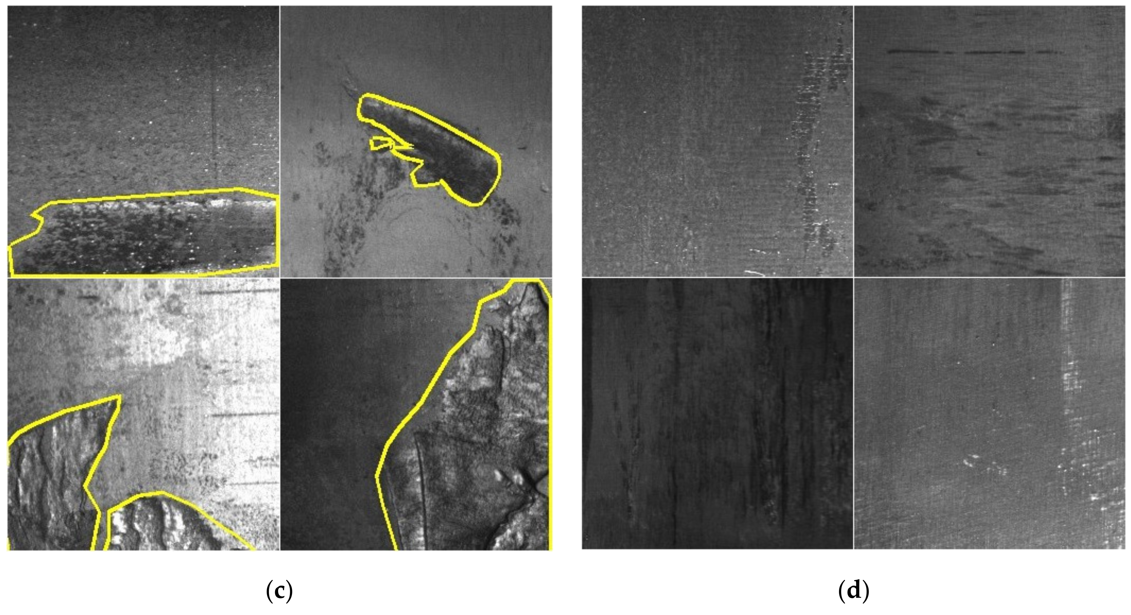
The neural network classifier was trained on a sample that contains 87,704 digital photos of flat steel surfaces with three types of damage, as well as images of undamaged surfaces (Figure 1). Training images are 256 × 256 pixels in size. A part of the images was taken from the Kaggle competition “Severstal: Steel Defect Detection” [35].
In total, the training sample contains 1820 images with class 1 damage, 14,576 images with class 2 damage, and 2327 images with class 3 damage. Some images show damage of several classes. In particular, there are 63 images with class 1 and 2 damage and 228 images with class 2 and 3 damage in the training image database. The training sample also contains 69,272 images of intact surfaces, which is 79% of its volume. The training sample is significantly unbalanced in terms of the distribution of different class images, which represent the distribution of classes in reality. This feature of the training sample requires using the relevant training techniques of the neural network, which reduces the impact of the input data heterogeneity [36,37]. Data imbalance negatively affects the outcome of training neural networks: the algorithm ignores small classes, which leads to low accuracy of classification. To solve the problem of data imbalance, the following methods were used:
  • applying class weights;
  • minority class over-sampling technique;
  • using focal loss function.
Class weights are designed to make the model pay more attention to classes that are less represented in the training sample. In practice, this was done using the tools of the Keras library. Weights are scalar coefficients to weight the loss contributions of different model outputs. The loss value that is minimized by the model will then be the weighted sum of all individual losses. However, in our case, the use of class weights did not give the desired positive effect.
Minority class over-sampling was performed by expanding the training sample with a number of training samples through augmentation [38,39]. The use of such an approach allowed us to train classifiers with an acceptable result. However, using the focal loss function allowed us to achieve the best results, so all the data presented in the article relate to classifiers with the focal loss function [40].
Focal loss applies a modulating term to the cross-entropy loss in order to focus training on hard negative examples. It down-weights the well-classified examples and puts more training emphasis on the data that is hard to classify. In a practical setting where we have a data imbalance, the majority class will quickly become well-classified since we have much more data for it. Thus, in order to ensure that we also achieve high accuracy for our minority class, we can use the focal loss to give those minority class examples more relative weight during training.
The surface of the steel samples under study has a different texture and shade, and the photos were obtained in different light conditions. Thus, the training sample is characterized by a significant variety not only of defects, but also of undamaged surfaces and the degree of their illumination. To form the best generalizing properties of the model, the input images were augmented. For this purpose, the data generator, which provided data for model training, flipped images relative to the horizontal and vertical axes and rotated them at an angle multiple of 90° with a certain probability. The technique of augmenting a training sample by means of image modification is widely used by researchers in various applied fields [38,39]. To achieve better generalization during validation, a validation image generator was used, which uses random augmentation. Given the random selection of transformations during the augmentation of each sample, we can state that for each epoch of learning, the validation subset of images will never be repeated. The OpenCV library was used for augmentation.
Although only three classes of surface defects have been selected for the study, the neural network classifier can easily be expanded by replacing the last fully connected layer of neurons.

4. Methodology

To solve the problem of classifying surface defects, residual neural networks were selected [41]. ResNet is one of the most powerful deep neural networks, which has shown excellent performance. Residual networks became the winner of ImageNet Large Scale Visual Recognition Challenge (ILSVRC) 2015 competition in image classification, detection, and localization, as well as the winner of Microsoft COCO: Common Objects in Context 2015 competition in detection and segmentation. The ILSVRC is an annual computer vision competition developed upon a subset of a publicly available computer vision dataset called ImageNet.
ResNet architecture allows building a very deep network of up to 1202 layers by training the residual representation functions instead of training the signal representation function [41,42]. ResNet introduces skip connection (or shortcut connection) to link the input from the previous layer to the next layer without any modification of the input. Instead of linking stacked layers to fit a desired underlying mapping, we explicitly let these layers fit a residual mapping. Skip connection makes it possible to have a deeper network and achieve better performance.
As part of solving the problem of classifying surface defects, we investigated residual neural networks ResNet34, ResNet50, ResNet152, and SeResNet50. Residual neural network ResNet50 was presented in 2015 by Microsoft Research command. ResNet50 demonstrates excellent generalization performance with fewer error rates on image recognition tasks and is, therefore, a useful tool for classification. Let us consider the structure of the classifier for detecting surface defects on the example of the basic model ResNet50. The classifier has 50 stacked layers and over 23 million trainable parameters. Xu et al. [38] argue that stacking layers should not degrade the network performance, because we could simply stack shortcut connections (layer that does not do anything) upon the current network, and the resulting architecture would perform the same.
The architecture of ResNet50 is shown in Figure 2. The model consists of four stages, each with a residual block. Each residual block has three layers that make 1 × 1 and 3 × 3 convolutions.
To reduce the problem of vanishing gradient in deeper layers, ResNet network uses shortcut connections. Shortcut connections transmit the input directly to the end of the residual block. ResNet50 model makes the initial convolution and max-pooling using 7 × 7 and 3 × 3 kernel sizes, respectively, with stride 2 in both cases. Then stage 1 of the network starts, which has three residual blocks containing three layers each. The kernel size, which was used to perform the convolution operation in all three layers of the block of stage 1, is 64, 64, and 256, respectively. As we go from one stage to another, the channel width is doubled, and the size of the input is reduced to half. The curved lines refer to the shortcut connection. The dashed curved lines represent convolution operation in the residual block that is performed with stride 2. Hence, the size of input will be reduced to half, but the channel width will be doubled.
As is shown in Figure 2, ResNet50 uses bottleneck design in its blocks. For each block, three layers are stacked one over another. The three layers are 1 × 1, 3 × 3, and 1 × 1 convolutions. The 1 × 1 convolution layers are reduced first, and then they restore the dimensions. The 3 × 3 layer is left as a bottleneck with smaller input/output dimensions.
It the end, the network has an average pooling layer followed by a fully connected layer with three neurons (by three classes of defects investigated). Each neuron may have a value in the range of [0…1] at the output, which can be considered as the model confidence in the presence of damage of a certain class in the input image.
The classifier is designed using Python 3.6 programming language with Keras and TensorFlow libraries.

5. Training

For training the classifier, we used transfer learning technique. As a base, we took ResNet50 trained on 1.4 million labeled images of 1000 classes from the ImageNet database.
All images were divided into the test group (20%) and the training group (the remaining 80%). While training the model, 20% of the training sample was used for validation. Damage of all classes is presented in each group in proportion to its share in the total amount.
Two types of classifiers—multilabel and multiclass—were studied. A multilabel classifier assumes that damage of several classes may be presented in a single image, while a multiclass classifier assumes that each image represents damage of only one class. Since in our case only 0.3% of images contains damage of several classes, we can presume that their total contribution to the error (in case of damage of only one class) will be insignificant. Previous research has shown that multilabel classifiers provide better accuracy. Therefore, only multilabel classifiers were investigated. Structurally, the multilabel classifier model is a combination of four binary classifiers. An individual threshold was used at the output of each of them to decide on the presence of damage of a certain class in the image analyzed. This made it possible to achieve optimal recognition quality for each class.
Binary loss functions and binary focal loss were used in training. At the end of each epoch, the values of the following metrics were preserved: false positives, false negatives, true positives, true negatives, accuracy, precision, recall, and area under receiver operating characteristic curve (AUC). It is established that the best result is achieved when using focal loss functions, which have proven themselves well for imbalanced data [37].
It was found during the previous research that the best results were achieved with the Stochastic Gradient Descent (SGD) optimizer and the focal loss function. The use of Adam and RMSprop optimizers led to a worse result. When training the classifier, hyperparameters such as training rate, batch size, and number of steps per epoch were varied.
The learning rate was initially set to 0.001 or 0.0005. After every 10 epochs, it was reduced by 25%, if the loss function did not improve. The batch size was set within 8–20 images during training. At the end of each epoch, the model was saved. Training was performed until the loss function improved over the last 10 epochs. As a result of training, a model was selected, for which the value of the validation loss function was the lowest. The training was conducted on a workstation with an Intel Core i7-2600 CPU, 32 GiB RAM and two NVIDIA GeForce GTX 1060 GPUs with 6 GiB of video memory.
In order to select the optimal classifier model, 29 models based on residual neural networks were studied. Hyperparameters of four of them are given in Table 2.
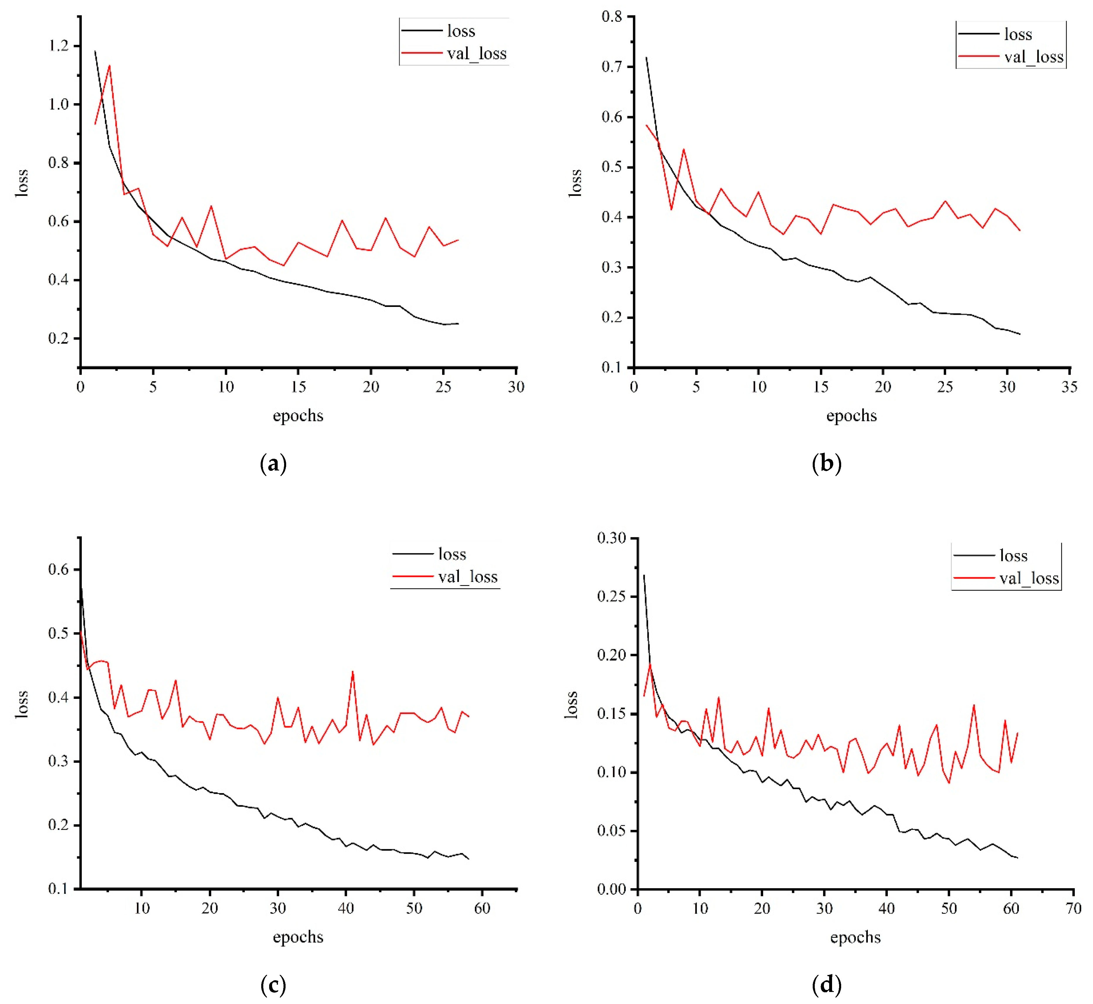
Variation graphs of binary focal loss function during training of classifiers from Table 2 are given in Figure 3. As is seen from the validation loss functions, the model attains the maximum level of data generalization over 20–40 epochs of training, after which overfitting comes gradually. At the same time, training losses continue decreasing.
The best result was shown by the model based on ResNet50, which was trained using the SGD optimizer with a moment of 0.9 at a learning rate of 0.001, batch size 20, and count of steps per epoch of 3000. Reducing the learning rate to 0.0005 slightly increased the duration of training but did not improve the result. Therefore, the value of 0.001 was chosen as optimal. Batch size within the range of 8–20 did not affect the result significantly.

6. Evaluation of Classifier Results and Discussion

To evaluate the classifier quality, we calculated the recall metrics, precision, F1 score, and binary accuracy for each classifier.
The recall metric shows what part of damage of a certain class is recognized correctly: R e c a l l = T P / T P + F N . The precision metric demonstrates which part of damage recognized as belonging to a particular class actually belongs to this class: P r e c i s i o n = T P / T P + F P .
The F1 score F 1 = 2 · P r e c i s i o n · R e c a l l / P r e c i s i o n + R e c a l l is an integrated metric and can be interpreted as a weighted average of the precision and recall, where an F1 score attains its best value at 1 and worst score at 0. The relative contributions of precision and recall to the F1 score are equal.
The binary accuracy metric shows the overall detection accuracy of all classes in the image.
The ground truth obtained at the output of the classifier during training has the form y g t = y 0 g t , y 1 g t , , y i g t , , y n c l 1 g t , where n c l is the number of classes (in our case, n c l = 3 ), y i g t is the output vector element, which is equal to 1, if the class with index i is present in the input image, and 0 if not.
The output prediction vector is y p r = y 0 p r , y 1 p r , , y i p r , , y n c l 1 p r where y i p r [0,1]. If the element of this vector is y i p r t b ( t b is a certain limit value), then a class with index i is present in the image, and vice versa. Let us denote a stepwise function that describes the following condition:
T b i n y i p r = 0 , y i p r < t b 1 , y i p r t b
We also denote the equality function of two arguments, which returns 1 if they are the same, and 0 otherwise:
E q x 1 , x 2 = 0 ,   x 1     x 2 1 ,   x 1 = x 2
Then the binary accuracy for one individual prediction is equal to:
a b i n 1 = 1 n c l i E q T b i n y i p r ,     y i g t .
Binary accuracy of batch prediction of input images with size n b :
a b i n = 1 n b j a b i n   j 1 .

6.1. Recall Metric

Class 2 damage was found to be the best recognized (for different models, recall ranges from 0.7102 to 0.7403). These damages are the most numerous and have a rather large area, which allows the model to acquire good generalizing properties. Class 3 damage is also well detected. It also has a large area and a sharp heterogeneity of morphology compared to the surrounding background. The recall metric ranges from 0.6169 to 0.6981 for different models of this class. The classifier is the worst at recognizing the finest damage of class 1, which is represented most scarcely in the training sample. For this class, recall is in the range of 0.2953 to 0.3509. All models detect undamaged surfaces best; for them, the recall is from 0.9392–0.9658. Undamaged images are most numerous (79% of the total) in the training sample, which allowed the model to learn their features best.
Thus, we can conclude that further expansion of the training sample, especially for damage of class 1, will allow training a model with the best generalizing properties.

6.2. Precision Metric

This metric is the best for class 3 damage, which is morphologically most different from background and other damage. Precision is in the range of 0.8714–0.8906 for this class. There are also quite a few false positives in the classification of class 2 damage. The precision metric is 0.8323–0.8561 for this class. The worst result is obtained for class 1 damage again: precision is in the range of 0.7131–0.8430. The number of false-positive cases is the smallest for undamaged surfaces (precision is 0.9401–0.9597).

6.3. F1 Score Metric

F1 score is an integrated metric that summarizes the values of recall and precision metrics. Since it is based on the values of the two previous metrics, it shows a similar result: class 1 damage is most poorly recognized (its metric is in the range of 0.4398–0.4706). Class 2 damage and class 3 damage are recognized much better: their metric reaches 0.7940 and 0.7809, respectively.

6.4. Binary Accuracy Metric

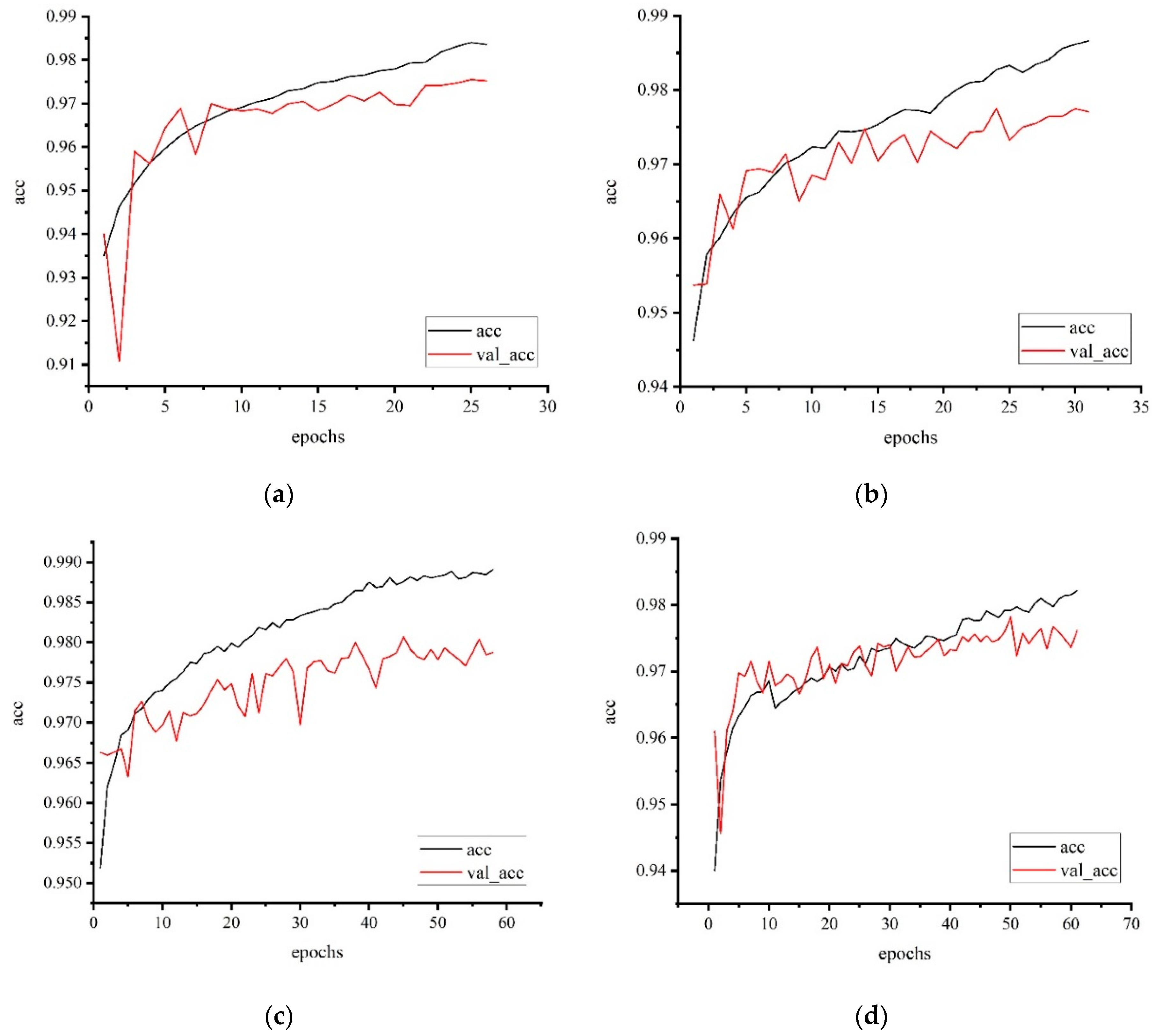
Binary accuracy calculates how often predictions match binary labels. Graphs of binary accuracy during training of different models are shown in Figure 4. For the test sample, the binary accuracy ranged from 0.9472 to 0.9691.
The value of the binary accuracy metric is affected both by the accuracy of determining the defect and the accuracy of determining the absence of defects in the image. Since classifiers can recognize the absence of defects very well, the value of the metric for all classes is high (0.9321–0.9884).
The analysis of the classification results showed that most false positives are associated with artifacts in the images that resemble real damage. Figure 5 shows images that do not have a defect but are incorrectly recognized as defective. Thus, in Figure 5, small artifacts can be seen (class 1 damage is represented by small spots but is actually a notch on the surface). Class 2 defects (scratches and scuffs) in the images have a different appearance, and one of them is represented by dark straight lines. Figure 5b illustrates the erroneous operation of the model on this type of surface formation. Class 3 damage is characterized by a large area and significant morphological diversity. In Figure 5c, we can see similar artifacts. Based on the results obtained, it can be assumed that a further expansion of the training sample will allow training a model with better characteristics, as this will provide the model with more features of the defects of each class.

6.5. Selecting the Best Model

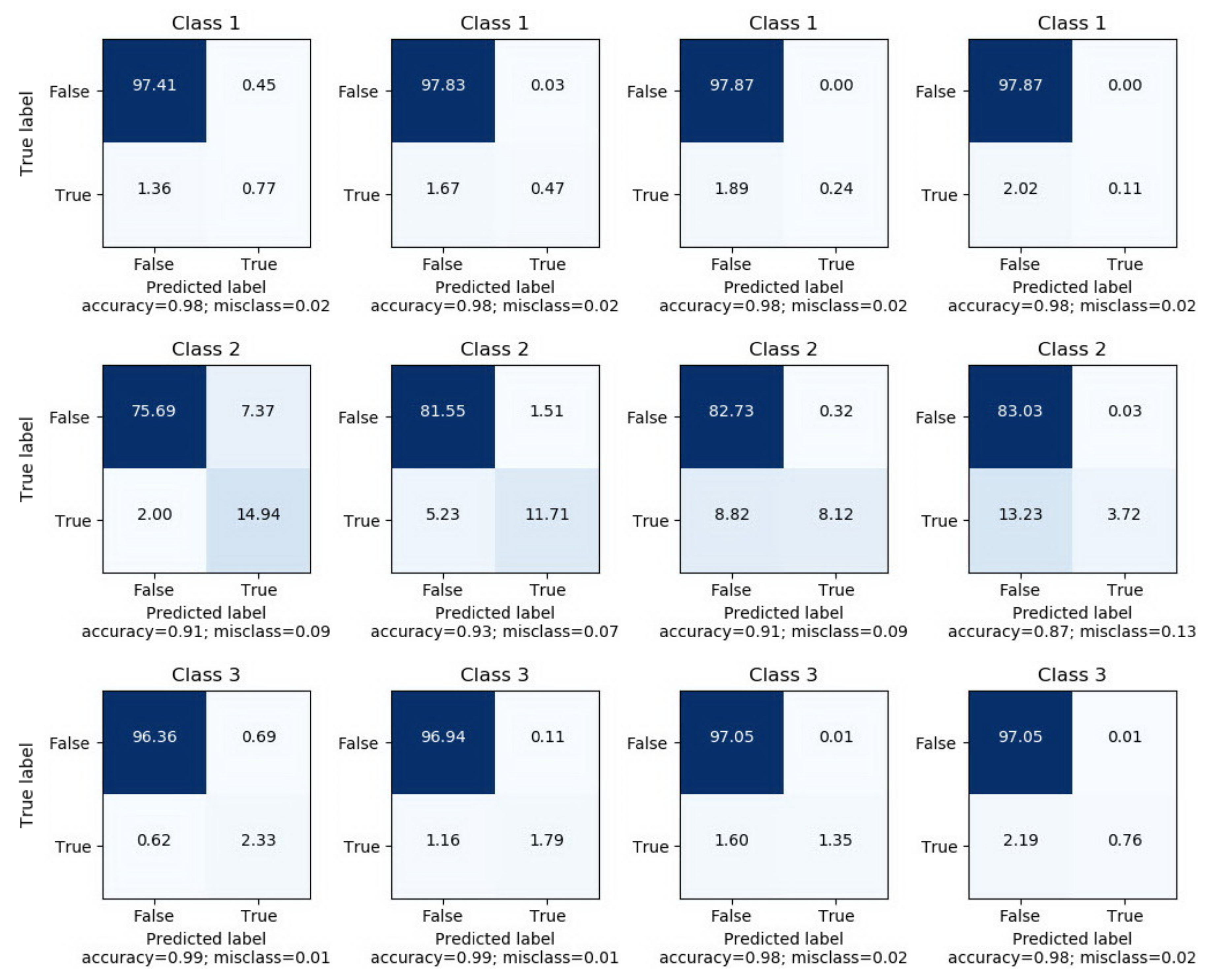
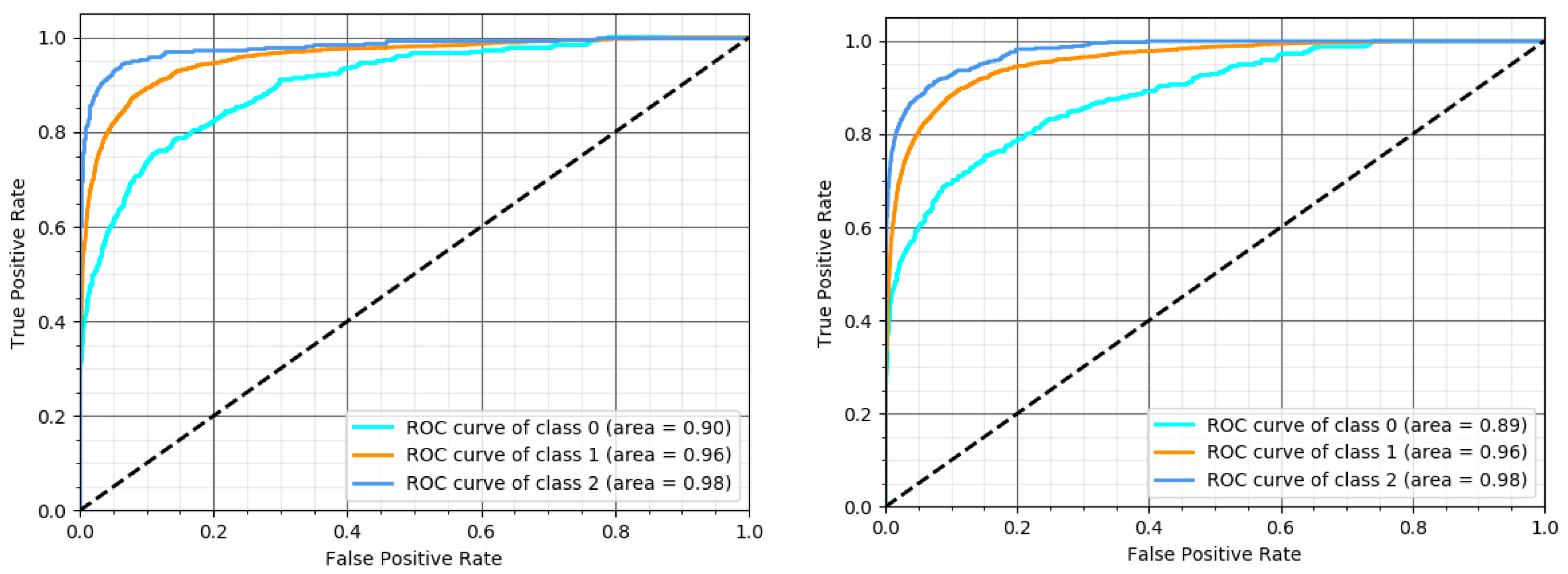
Since each output neuron of the model yields a result that does not depend on the values of other neurons, each class of defects may have its own optimal threshold, at which the best performance will be achieved. Therefore, the classification result for thresholds from 0 to 1 with a step of 0.05 was analyzed for each class. The confusion matrix of model 1 for each class, which shows the proportion of samples recognized correctly and incorrectly at threshold 0.2, 0.4, 0.6, and 0.8, is shown in Figure 6. The upper left cell of each matrix (true negatives) corresponds to the correctly recognized undamaged surfaces, which are most numerous. The lower right cell (true positives) corresponds to correctly classified images with defects of the corresponding class. Two other cells (false positive and false negative) correspond to type I and type II errors. The goal is to find a threshold for each class that will yield a minimum number of errors. This is convenient to do with receiver operating characteristic (ROC) curves.
The ROC curve demonstrates the ability of the binary classifier to recognize the input signal at different thresholds of the output signal. The curve shows the dependence of true positive rate ( T P R = T P / T P + F N ) on false positive rate ( F P R = F P / F P + T N ) at different thresholds. ROC curves are insensitive to class distribution. If the proportion of positive to negative instances changes, the ROC curve will not change. The area under this curve (AUC-ROC) is an integral indicator of the model quality, which summarizes its ability to distinguish a particular class.
Figure 7 shows the ROC curves for model 1 from Table 2. The AUC-ROC area for different classes is 0.90–0.98. As seen from the graphs, class 3 damage (AUC-ROC area is 0.98), which is characterized by significant morphological differences compared to undamaged surfaces, is best identified. Class 2 damage is also well recognized (AUC-ROC area is 0.96). Fine damage of class 1 that often merges with the background (the lowest AUC-ROC area of 0.90) is the most difficult to detect.
After analyzing the results of the model at different thresholds, we chose the optimal limit value for each class, which provided the best accuracy of classification. Table 3 shows the performance metrics of the most successful models for the optimal threshold.
The most problematic in terms of detection are objects of class 1. Different models show somewhat different abilities to detect damage of different types. Thus, model 2 detects class 1 defects 16% better than model 1, but shows a much greater number of false positives, as indicated by the precision metric (0.7143 vs. 0.8430). As a result, the overall accuracy of model 1 is higher for this class. The results of different models are very similar for class 2 and class 3 damage, which are better represented in the training sample. According to the generalized metric F1 score, model 1 is the best.

7. Conclusions

A number of classification models based on deep residual neural networks were constructed, and their qualitative metrics investigated on the images of flat surfaces of rolled metal. The results showed that the proposed models can be used to detect surface defects with high accuracy. Defects with a sufficiently large area (class 2 and 3) are best identified. Fine damage of class 1, which is most similar to surface formations often found on intact specimens, is the most difficult to recognize. At the same time, it seems possible to significantly improve the results for class 1 damage. It requires expanding the training sample of photos of damage in this class.
Examining the results of different types of ResNet models, we found that the optimal depth of the model was 50 layers. Simpler models (34 layers) showed worse generalizing properties, while deeper models showed better results at training. However, the results were worse on the test data, indicating overfitting (or insufficient training sample for complex models).
The best model of the multilabel classifier based on ResNet50 showed an average accuracy of classification of 0.9691 for all types of damage. The model was trained using the binary focal loss function and the SGD optimizer.

Author Contributions

Conceptualization, P.M.; formal analysis, I.K.; investigation, I.K., P.M., J.B. (Janette Brezinová), and J.V.; methodology, I.K.; project administration, J.B. (Janette Brezinová); validation, I.K., P.M., J.B. (Jakub Brezina), and J.V.; visualization, I.K., J.B. (Jakub Brezina); writing—original draft, I.K. and P.M.; writing—review and editing, J.B. (Jakub Brezina) and J.V. All authors have read and agreed to the published version of the manuscript.

Funding

This research was funded by Ministry of Education of the Slovak Republic VEGA No. 1/0424/17, KEGA 001STU-4/2019, and the Slovak Research and Development Agency APVV-16-0359. The APC was funded by the Slovak Research and Development Agency.

Acknowledgments

This work was supported by scientific grant agency of the Ministry of Education of the Slovak Republic VEGA No. 1/0424/17, KEGA 001STU-4/2019, and the Slovak Research and Development Agency APVV-16-0359.

Conflicts of Interest

The authors declare no conflict of interest.

References

  1. Mazur, I.P. Monitoring the surface quality in sheet rolling. Steel Transl. 2011, 41, 326–331. [Google Scholar] [CrossRef]
  2. Mazur, I.; Koinov, T. Quality control system for a hot-rolled metal surface. Frattura ed Integrità Strutturale 2016, 37, 287–296. [Google Scholar] [CrossRef] [Green Version]
  3. Kostenetskiy, P.; Alkapov, R.; Vetoshkin, N.; Chulkevich, R.; Napolskikh, I.; Poponin, O. Real-time system for automatic cold strip surface defect detection. FME Trans. 2019, 47, 765–774. [Google Scholar] [CrossRef] [Green Version]
  4. Neogi, N.; Mohanta, D.K.; Dutta, P.K. Review of vision-based steel surface inspection systems. EURASIP J. Image Video Process. 2014, 2014, 50. [Google Scholar] [CrossRef] [Green Version]
  5. Yun, J.P.; Choi, S.H.; Jeon, Y.-J.; Choi, D.-C.; Kim, S.W. Detection of line defects in steel billets using undecimated wavelet transform. In Proceedings of the International Conference on Control, Automation and Systems (ICCAS ’08), Seoul, South Korea, 14–17 October 2008; pp. 1725–1728. [Google Scholar]
  6. Zhao, Y.J.; Yan, Y.H.; Song, K.C. Vision-based automatic detection of steel surface defects in the cold rolling process: Considering the influence of industrial liquids and surface textures. Int. J. Adv. Manuf. Technol. 2017, 90, 1665–1678. [Google Scholar] [CrossRef]
  7. Liu, Y.; Hsu, Y.; Sun, Y.; Tsai, S.; Ho, C.; Chen, C. A computer vision system for automatic steel surface inspection. In Proceedings of the Fifth IEEE Conference on Industrial Electronics and Applications, Taichung, Taiwan, 15–17 June 2010; pp. 1667–1670. [Google Scholar]
  8. Agarwal, K.; Shivpuri, R.; Zhu, Y.; Chang, T.; Huang, H. Process knowledge based multi-class support vector classification (PK-MSVM) approach for surface defects in hot rolling. Expert Syst. Appl. 2011, 38, 7251–7262. [Google Scholar] [CrossRef]
  9. Wang, T.; Chen, Y.; Qiao, M.; Snoussi, H. A fast and robust convolutional neural network-based defect detection model in product quality control. Int. J. Adv. Manuf. Technol. 2018, 94, 3465–3471. [Google Scholar] [CrossRef]
  10. Zhou, S.; Chen, Y.; Zhang, D. Classification of surface defects on steel sheet using convolutional neural networks. Mater. Technol. 2017, 51, 123–131. [Google Scholar] [CrossRef]
  11. GOST 21014-88. Rolled Products of Ferrous Metals. Surface Defects. Terms and Definitions; Izd. Stand.: Moscow, USSR, 1989; p. 61. (In Russian) [Google Scholar]
  12. Bernshteyn, M.L. (Ed.) Atlas Defects of Steel; Metallurgiya: Moscow, USSR, 1979; p. 188. (In Russian) [Google Scholar]
  13. Becker, D.; Bierwirth, J.; Brachthäuser, N.; Döpper, R.; Thülig, T. Zero-Defect-Strategy in the Cold Rolling Industry. Possibilities and Limitations of Defect Avoidance and Defect Detection in the Production of Cold-Rolled Steel Strip; Fachvereinigung Kaltwalzwerke e.V., CIELFFA: Düsseldorf, Germany, 2019; p. 16. [Google Scholar]
  14. Hu, H.; Li, Y.; Liu, M.; Liang, W. Classification of defects in steel strip surface based on multiclass support vector machine. Multimed. Tools Appl. 2014, 69, 199–216. [Google Scholar] [CrossRef]
  15. Sun, X.; Gu, J.; Tang, S.; Li, J. Research progress of visual inspection technology of steel products—A Review. Appl. Sci. 2018, 8, 2195. [Google Scholar] [CrossRef] [Green Version]
  16. Zhao, C.; Zhu, H.; Wang, X. Steel plate surface defect recognition method based on depth information. In Proceedings of the IEEE 8th Data Driven Control and Learning Systems Conference (DDCLS), Dali, China, 24–27 May 2019; pp. 322–327. [Google Scholar]
  17. Ma, Y.; Li, Q.; Zhou, Y.; He, F.; Xi, S. A surface defects inspection method based on multidirectional gray-level fluctuation. Int. J. Adv. Robot. Syst. 2017, 14, 109–125. [Google Scholar] [CrossRef] [Green Version]
  18. Song, G.; Song, K.; Yan, Y. Saliency detection for strip steel surface defects using multiple constraints and improved texture features. Opt. Lasers Eng. 2020, 128, 106000. [Google Scholar] [CrossRef]
  19. Fu, G.; Sun, P.; Zhu, W.; Yang, J.; Cao, Y.; Yang, M.Y.; Cao, Y. A deep-learning-based approach for fast and robust steel surface defects classification. Opt. Lasers Eng. 2019, 121, 397–405. [Google Scholar] [CrossRef]
  20. Song, K.; Yan, Y. A noise robust method based on completed local binary patterns for hot-rolled steel strip surface defects. Appl. Surf. Sci. 2013, 285, 858–864. [Google Scholar] [CrossRef]
  21. Liu, Y.; Geng, J.; Su, Z.; Zhang, W.; Li, J. Real-Time Classification of Steel Strip Surface Defects Based on Deep CNNs. In Lecture Notes in Electrical Engineering, Proceedings of 2018 Chinese Intelligent Systems Conference; Jia, Y., Du, J., Zhang, W., Jia, Y., Zhang, W., Eds.; Springer: Berlin, Germany, 2019; p. 529. [Google Scholar] [CrossRef]
  22. Tao, X.; Zhang, D.; Ma, W.; Liu, X.; Xu, D. Automatic metallic surface defect detection and recognition with convolutional neural networks. Appl. Sci. 2018, 8, 1575. [Google Scholar] [CrossRef] [Green Version]
  23. Kim, M.S.; Park, T.; Park, P. Classification of Steel Surface Defect Using Convolutional Neural Network with Few Images. In Proceedings of the 12th Asian Control Conference (ASCC), Kitakyushu-shi, Japan, 9–12 June 2019; pp. 1398–1401. [Google Scholar]
  24. Yasniy, P.V.; Maruschak, P.O. Continuous Casting Machine Rollers: Degradation and Crack Resistance; Dzhura: Ternopil, Ukraine, 2009; p. 232. (In Ukrainian) [Google Scholar]
  25. Brezinová, J.; Viňáš, J.; Maruschak, P.; Guzanová, A.; Draganovská, D.; Vrabeľ, M. Sustainable Renovation within Metallurgical Production; RAM-Verlag: Lüdenscheid, Germany, 2017; p. 215. [Google Scholar]
  26. Brezinová, J.; Viňáš, J.; Brezina, J.; Guzanová, A.; Maruschak, P. Possibilities for renovation of functional surfaces of backup rolls used during steel making. Metals 2020, 10, 164. [Google Scholar] [CrossRef] [Green Version]
  27. Masci, J.; Meier, U.; Ciresan, D.; Schmidhuber, J.; Fricout, G. Steel defect classification with Max-Pooling Convolutional Neural Networks. In Proceedings of the International Joint Conference on Neural Networks (IJCNN), Brisbane, QLD, Australia, 10–15 June 2012; pp. 1–6. [Google Scholar] [CrossRef] [Green Version]
  28. Lee, S.Y.; Tama, B.A.; Moon, S.J.; Lee, S. Steel Surface Defect Diagnostics Using Deep Convolutional Neural Network and Class Activation Map. Appl. Sci. 2019, 9, 5449. [Google Scholar] [CrossRef] [Green Version]
  29. Mohan, A.; Poobal, S. Crack detection using image processing: A critical review and analysis. Alex. Eng. J. 2018, 57, 787–798. [Google Scholar] [CrossRef]
  30. Gao, Y.; Gao, L.; Li, X.; Yan, X. A semi-supervised convolutional neural network-based method for steel surface defect recognition. Robot. Comput. Integr. Manuf. 2020, 61, 101825. [Google Scholar] [CrossRef]
  31. Di, H.; Ke, X.; Peng, Z.; Dongdong, Z. Surface defect classification of steels with a new semi-supervised learning method. Opt. Lasers Eng. 2019, 117, 40–48. [Google Scholar] [CrossRef]
  32. Cui, W.; Zhang, Y.; Zhang, X.; Li, L.; Liou, F. Metal Additive Manufacturing Parts Inspection Using Convolutional Neural Network. Appl. Sci. 2020, 10, 545. [Google Scholar] [CrossRef] [Green Version]
  33. Liu, Y.; Xu, K.; Xu, J. An improved MB-LBP defect recognition approach for the surface of steel plates. Appl. Sci. 2019, 9, 4222. [Google Scholar] [CrossRef] [Green Version]
  34. Li, Y.; Li, G.; Jiang, M. An end-to-end steel strip surface defects recognition system based on convolutional neural networks. Steel Res. Int. 2017, 88, 60–68. [Google Scholar]
  35. Kaggle Severstal: Steel Defect Detection. Can You Detect and Classify Defects in Steel? 2019. Available online: https://www.kaggle.com/c/severstal-steel-defect-detection (accessed on 25 June 2020).
  36. He, H.; Garcia, E.A. Learning from Imbalanced Data. IEEE Trans. Knowl. Data Eng. 2009, 21, 1263–1284. [Google Scholar]
  37. Frasca, M.; Bertoni, A.; Re, M.; Valentini, G. A neural network algorithm for semi-supervised node label learning from unbalanced data. Neural Netw. 2013, 43, 84–98. [Google Scholar] [CrossRef] [Green Version]
  38. Xu, Y.; Jia, R.; Mou, L.; Li, G.; Chen, Y.; Lu, Y.; Jin, Z. Improved Relation Classification by Deep Recurrent Neural Networks with Data Augmentation. arXiv 2016, arXiv:1601.03651. [Google Scholar]
  39. Zhong, Z.; Zheng, L.; Kang, G.; Li, S.; Yang, Y. Random Erasing Data Augmentation. arXiv 2017, arXiv:170804896. [Google Scholar] [CrossRef]
  40. Lin, T.-Y.; Goyal, P.; Girshick, R.; He, K.; Dollár, P. Focal Loss for Dense Object Detection. arXiv 2017, arXiv:1708.02002v2. [Google Scholar]
  41. He, K.; Zhang, X.; Ren, S.; Sun, J. Deep Residual Learning for Image Recognition. arXiv 2015, arXiv:1512.03385v1. [Google Scholar]
  42. Jain, V.; Patnaik, S.; Popențiu Vlădicescu, F.; Sethi, I.K. Recent Trends in Intelligent Computing, Communication and Devices. In Proceedings of the ICCD 2018; Springer Nature: Singapore, 2020. [Google Scholar]
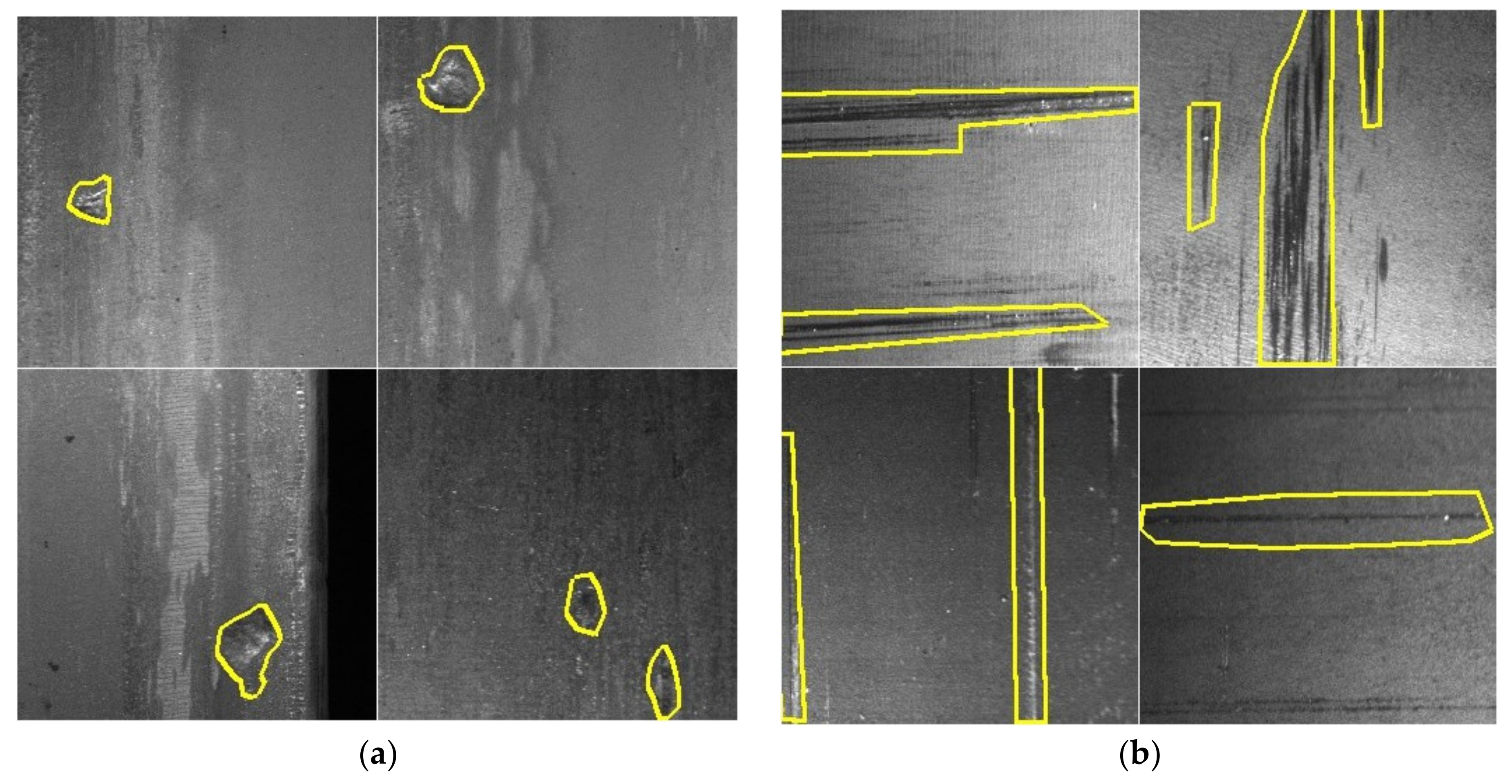
Figure 1. Images with class 1 (a), class 2 (b), and class 3 (c) damage. See Table 1 and images of undamaged surfaces (d).
Metals 10 00846 g001aMetals 10 00846 g001b
Figure 2. ResNet50 classifier architecture.
Metals 10 00846 g002
Figure 3. Training curves of classifier models from Table 2: (a) model 1, (b) model 2, (c) model 3, and (d) model 4.
Metals 10 00846 g003
Figure 4. Curves of binary accuracy during training of classifier models from Table 2: (a) model 1, (b) model 2, (c) model 3, and (d) model 4.
Metals 10 00846 g004
Figure 5. False positives for damage of class 1 (a), class 2 (b), and class 3 (c), respectively.
Metals 10 00846 g005aMetals 10 00846 g005b
Figure 6. Confusion matrix of model 1 for three classes of defects at different thresholds. In each row, the matrices are obtained for the thresholds 0.2, 0.4, 0.6, and 0.8, respectively.
Metals 10 00846 g006
Figure 7. Receiver operating characteristic (ROC) curves of classifiers with the best quality metrics (models 1 and 2, Table 2).
Metals 10 00846 g007
Table 1. Defectoscopic signs of defects.
ClassDefect FeaturesDefect TypeReasons for OccurrenceAutomatic Inspection of the StripPrevention
1Single and multiple defects in the form of rounded spots.HolesHoles can occur as a result of inclusions directly under the surface. Such inclusions are stretched by subsequent deformation or are rolled over.PossibleLimitation of the scatter of melting metallurgy and casting parameters.
2Multiple linear and elongated defects of any orientation throughout the surface of rolled metal.Grooves/ScratchesThese forms of damage occur as a consequence of relative movements between the rolled product and parts of the installation.PossiblePreventive measures to avoid mechanical damage. Preventive maintenance.
3Surface defects, which are peeling of a metal of a tongue-like shape. With separation of exfoliation, a deep depression with an uneven bottom is formed.RollingWear of the rollers.PossibleRegular change of rolls according to wear behavior.
Table 2. Hyperparameters of classifier models.
NumberBase ModelDescription
1ResNet50batch_size = 20, lr = 0.001,
steps_per_epoch = 3000, validation_steps = 1000
2ResNet50batch_size = 16, lr = 0.0005,
steps_per_epoch = 2000, validation_steps = 700
3SeResNet50batch_size = 16, lr = 0.001,
steps_per_epoch = 3000, validation_steps = 1000
4ResNet152batch_size = 8, lr = 0.001,
steps_per_epoch = 2000, validation_steps = 7000
Table 3. Performance metrics of model 1 and model 2.
ClassThresholdTPTNFPFNRecallPrecisionAccuracyF1 Score
Model 1
10.2751021548192360.30180.84300.98390.4445
20.350198712,8223346970.74030.85610.93490.7940
30.29532615,331421410.69810.88590.98840.7809
Model 2
10.12012015,450482220.35090.71430.98300.4706
20.405196012,8053677080.73460.84230.93210.7848
30.19028515,343351770.61690.89060.98660.7289