Abstract
Bainite is an essential constituent of modern high strength steels. In addition to the still great challenge of characterization, the classification of bainite poses difficulties. Challenges when dealing with bainite are the variety and amount of involved phases, the fineness and complexity of the structures and that there is often no consensus among human experts in labeling and classifying those. Therefore, an objective and reproducible characterization and classification is crucial. To achieve this, it is necessary to analyze the substructure of bainite using scanning electron microscope (SEM). This work will present how textural parameters (Haralick features and local binary pattern) calculated from SEM images, taken from specifically produced benchmark samples with defined structures, can be used to distinguish different bainitic microstructures by using machine learning techniques (support vector machine). For the classification task of distinguishing pearlite, granular, degenerate upper, upper and lower bainite as well as martensite a classification accuracy of 91.80% was achieved, by combining Haralick features and local binary pattern.
1. Introduction
Bainite is a typical constituent of modern high strength steels, combining high strength and high toughness and thereby making it interesting for many applications. In order to adjust desired strength or toughness levels in these steels, it is essential to know and understand what types of bainite are present depending on chemical composition and processing steps. The characterization or classification of bainite, however, is a difficult task because of the variety and amount of involved phases as well as the fineness and complexity of the structures. Moreover, the lack of consensus among human experts in labeling and classifying bainitic structures further complicates this task.
There is also no consistent nomenclature to describe or label bainitic microstructures, and many different classification schemes can be found in literature. There are two concepts for classification schemes, the first is to describe the arrangement of ferrite and carbon-rich phase as a whole, using one integral expression. The oldest and most common known descriptions of this kind are upper and lower bainite [1]. Other existing classification schemes were suggested by Ohmori et al. [2], Bramfitt and Speer [3] or by Lotter and Hougardy [4] and Aaronson et al. [5]. Furthermore, summaries of several classification schemes can be found in [5] and [6]. One of the most well-known schemes is proposed by Zajac et al. [7]. Five different bainitic structures are distinguished. Their schematic structures are shown in Figure 1. Upper bainite consists of lath-like ferrite with cementite on the lath boundaries. Instead of cementite, degenerated upper bainite has so-called martensite-retained austenite constituents [1] (MA) on the lath boundaries. Lower bainite consists of lath-like ferrite with cementite precipitated inside the ferrite laths. Degenerated lower bainite is again with MA constituents instead of cementite. Granular bainite is defined as irregular ferrite with carbon-rich second phases distributed between these irregular grains. Typically, the carbon-rich second phase is not cementite, but any transformation product that can develop from carbon-enriched austenite. They investigated five types of second phases: (i) degenerated pearlite or debris of cementite, (ii) bainite, (iii) mixture of “incomplete” transformation products, (iv) MA, and (v) martensite. The advantage of this scheme is that it covers various bainitic microstructures and can be easily used and understood in common parlance.
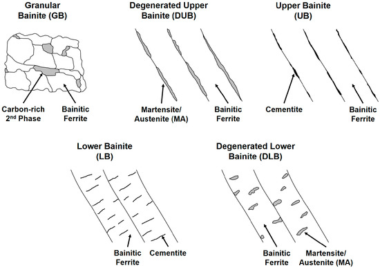
Figure 1.
Schematics of the 5 bainite types suggested by Zajac [7]. Diagram is modified according to [7].
The second concept for bainite classification is to describe the ferritic and the carbon-rich phase separately. This has been done in [8,9,10,11]. For example, in Gerdemann [9], the ferritic phase is described by its crystallographic structure and morphology and the secondary phase by its location, crystallographic structure, and morphology. From these descriptions, certain letters are taken to write an abbreviation for the microstructure. With this classification concept it is more of a pure description of the microstructure without the subjective component of pressing it into one integral expression. However, those coded descriptions are hard to use in common speech.
Considering the aforementioned challenges when dealing with bainite, it is not surprising that not many approaches for an automated classification of steel microstructures, including bainite subclasses can be found in the literature. Gola et al. [12] used a combination of morphological and textural parameters with a support vector machine (SVM) to classify the carbon-rich second phase of two phase steels into pearlite, bainite, and martensite. However, bainite subclasses were not considered, as all structures that were neither pearlite nor martensite were put into one bainite class. Azimi et al. [13] worked with the same data set, but used deep learning methods for classification of pearlite, bainite, martensite, and tempered martensite, however, bainite subclasses were also not included. Zajac et al. [14] use misorientation angle distribution from electron backscatter diffraction (EBSD) measurements to differentiate granular, upper and lower bainite. Tsuitsui et al. [15] used misorientation parameters and variant pairs from EBSD data to distinguish bainite formed at high and low temperatures as well as martensite and bainite–martensite mixtures. Komenda et al. [16] used trainable segmentation to distinguish ferrite, pearlite, martensite, upper and lower bainite in sintered steel, however the segmentation result is shown in a light optical microscope picture and differences between martensite, lower and upper bainite are not discussed in detail. In Miyama et al. [17] upper and lower bainite are distinguished by calculating morphological parameters of the cementite precipitates. Banerjee et al. [18] differentiate ferrite, bainite, and martensite by using intensity values as well as density of substructure particles, whereas Paul et al. [19] use regional contour pattern and local entropy to segment ferrite, martensite and bainite in dual-phase-steels. Regarding the suggested classifications schemes for bainite mentioned earlier, there are no reported automated workflows who use the differences cited in the definition of these bainite classes for a classification task.
The analysis of the texture of an image is a promising way to distinguish images in general but also steel microstructure images. Image texture is the “spatial arrangement of color or intensities in an image” [20]. Image texture based analysis methods include Haralick textural parameters [21] and local binary patterns [22], amongst others. Webel et al. [23] developed a new approach based on Haralick textural parameters. Instead of calculating the parameters only at angles of 0°, 45°, 90°, and 135°, they are calculated from the 1° stepwise rotation of images, making the values independent of the original texture orientation. By doing this, they were able to distinguish pearlite, lower bainite, and martensite. Local binary pattern are for example used in [24] to distinguish phases in ferrite–pearlite and martensite–austenite microstructures.
In order to use a machine learning classification approach, it is important to assign the ground truth in the most objective way. When dealing with complex microstructures this can be challenging. One way to make the ground truth assignment more objective is to use reference samples where there is no doubt about the present microstructures. In this work, bainitic reference samples are used and analyzed based on the workflows suggested by Webel et al. and Gola et al., which is feature extraction by using Haralick textural parameters, now also complemented by using local binary pattern, followed by machine learning classification using a support vector machine, in order to demonstrate the feasibility of a classification of bainite subclasses.
2. Materials and Methods
2.1. Material
The assignment of the ground truth for machine learning classification has a subjective component that should not be underestimated. Industrial steel samples usually exhibit complex microstructures, with bainitic phase constituents often being small or inhomogeneous. This makes it difficult to extract ground truth parameters from these regions in an objective and statistically secured way. For this reason, samples were specifically produced using a quenching dilatometer (TA Instruments 805 A/D, TA Instruments, New Castle, DE, USA, Hüllhorst, Germany) to obtain bainitic microstructures. Sample material was taken from an industrial steel grade, capable of achieving a typical yield strength range of 1050–1250 MPa, after hot rolling and heat treatment. The carbon content of the material is 0.22 wt.%, alloying elements are manganese, chromium and nickel as well as microalloying additions Nb, Ti, and B, see Table 1. Because of industrial collaboration, exact microalloying amounts cannot be given. This composition was chosen after extensive review of literature about bainitic steels and correlations to their chemistry and processing conditions. E.g. in Zajac et al. [14] similar steel compositions (steel group “II”) yielded predominant bainitic structures and also allowed to adjust different bainite types, including lower bainite which typically doesn’t form in low-carbon steels, depending on the cooling rate.

Table 1.
Chemical composition of the used steel, in weight %.
Samples with a diameter of 4 mm and length of 10 mm were machined for use in the quenching dilatometer. After identical austenitization at 1000 °C for 10 min, samples were continuously cooled with different cooling rates, ranging from 2 K/s to the maximum cooling rate of 278 K/s, in order to get different bainitic microstructures (Figure 2).
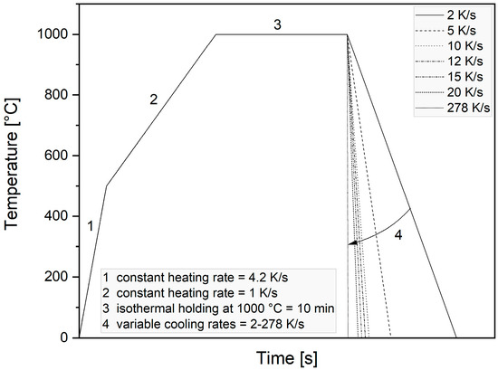
Figure 2.
Time–temperature-profile of sample production experiments: after heating (1,2) samples are austenitized at 1000 °C for 10 min (3), and then continuously cooled with varying cooling rates (4).
2.2. Sample Preparation
The samples were ground using 80–1200 grid SiC papers and then subjected to 6, 3, and finally, 1 μm diamond polishing to obtain smooth surfaces for subsequent etching. Metallographic etching was carried out by submerging polished sample surfaces into a mixture of ethanol and nitric acid (2 vol. %), also called “Nital” etching.
2.3. Microscopy
Each sample was imaged in a scanning electron microscope (Supra FE-SEM, Carl Zeiss Microscopy GmbH, Jena, Germany) using secondary electron contrast at a magnification of 2000× with an image size of 2048 × 1536 pixels. SEM was operated at an acceleration voltage of 5 kV, an aperture of 30 µm to set the probe current and a working distance of 5 mm. To get reference images with just one phase constituent and to avoid any potential heterogeneities, the captured images were later cropped to 350 × 350 px, equal to 9.70 × 9.70 µm. During image acquisition, care was taken not to cut off the greyscale histogram. Also, because the image contrast depends on the intensity of etching and sample preparation, all images were subsequently normalized regarding their gray value histogram.
2.4. Calculation of Haralick Parameters
The textural parameters developed by Haralick et al. [21] essentially describe how often a gray value appears in the image in a certain spatial relationship to another gray value. For this, the gray level co-occurrence matrix (GLCM) of the image is calculated. From the GLCM several parameters representing the image texture can be calculated. This is illustrated in Figure 3.
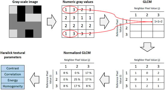
Figure 3.
Visualization of calculation of Haralick Parameters: input is a gray-scale image from which the gray level co-occurrence matrix (GLCM) is calculated. Using mathematical matrix operations, different parameters like contrast, correlation, energy and homogeneity can be calculated from the GLCM. Diagram is modified according to [25].
While the original approach of Haralick’s analysis measures the pairing of gray values only for directions at angles of 0°, 45°, 90°, and 135°, the approach presented by Webel et al. [23] where the image is rotated in 1° steps from 0° to 180° and the GLCM is measured for each rotation, is used in this work. From these rotations the mean value as well as the amplitude, defined as maximum minus minimum, of the textural parameters are calculated. This is done using MATLAB (R2019b, MathWorks, Natick, MA, USA) and the built-in functions for Haralick Parameters. Here, the Haralick parameters contrast, correlation, energy and homogeneity are used. By using averaged parameters of the rotation, these parameters become rotation invariant. For more detailed descriptions, the author refer to [21,23].
2.5. Calculation of Local Binary Pattern
Local Binary Pattern (LBP) is a texture descriptor, originally made by Ojala et al. [22]. LBP features encode the neighboring context of each pixels into a histogram of the whole image which is used as final feature descriptor. The process of calculating LBP features is visualized in Figure 4. For further details the authors refer to the original publication by Ojala et al. [22]. LBP features can be calculated by using different parameters for the neighborhood, that’s the number of neighboring pixels (N) and the distance of the neighboring pixels (R) that are considered. By considering a circular neighborhood instead of a square, LBP features become rotation invariant. The main advantage of LBP is that it can easily encode fine details in the structure. However, as the encoding happens in a small scale it cannot capture large textures. In [26], multi-scale LBP were introduced to address this problem. Multi-scale LBP are created by simply concatenating LBP features with different neighboring parameters N and R. In this work, uniform, rotation invariant LBP with histogram normalization are used. Calculation was done in MATLAB (R2019b, MathWorks, Natick, MA, USA) with an open-source code for LBP. Neighboring parameters of R = 1 and N = 8 (1/8), 2.4/8, 4.2/16, and 6.2/16 are used for single-scale LBP. Additionally, all those four scales are combined into a multi-scale LBP.
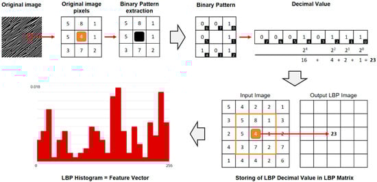
Figure 4.
Visualization of calculation of Local Binary Pattern (LBP): An example region of the original image is examined, with neighboring parameters of R = 1 and N = 8. Neighboring pixels are compared to the center pixel: pixel values smaller than the center pixel values are assigned to 1, pixel values bigger to 0. Binary values are stringed together. This allows a calculation of a decimal value which will be stored in matrix with the same width and height as the original image and in the same place as the input center pixel. This is done for every pixel of the image. The LBP matrix can be represented as a histogram which will be treated as the feature vector of the original image.
2.6. Classification Process Using Support Vector Machine
For classification, the workflow presented by Gola et al. [12,27], using a support vector machine (SVM) was adopted. An SVM classifies data by finding the best hyperplane that separates the data points of one class from the data points of another class. The implementation was done using MATLAB (R2019b, MathWorks, Natick, MA, USA) classification learner app, which allows automated classifier training of different SVM in order to find its best kernel and parameter settings. To estimate the predictive accuracy 5-fold cross-validation was used. Following parameters of the SVM, that are available in MATLAB classification learner app, that were kept constant are a box constraint level of 1, auto kernel scale mode, one-vs-one multiclass method and data standardization.
3. Results
3.1. Microstructures
Figure 5 shows a continuous cooling diagram where regions for the specific microstructures are marked. Table 2 lists the microstructure constituents found in each sample. Corresponding images, before cropping for further analysis, are shown in Supplemental Figures S1–S4.
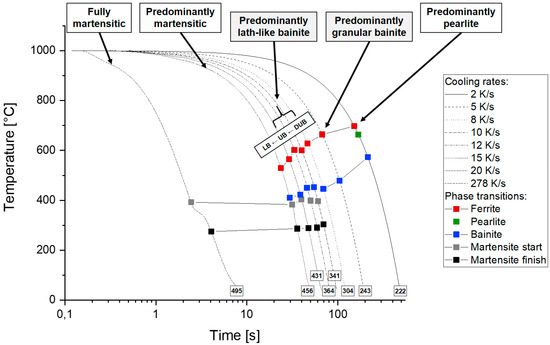
Figure 5.
Continuous cooling diagram showing different cooling rates after austenitization at 1000 °C, phase transitions of ferrite, pearlite, bainite, and martensite. Additionally, regions where different microstructures predominantly formed are shown. Also, measured hardness values (HV1) for each cooling rate are added.
Table 2.
List of microstructures found in the produced samples.
The captured images from these samples were cropped to 350 × 350 px, equal to 9.70 × 9.70 µm, to get reference images with just one microstructure class. To label the bainitic structures present in the samples, the classification scheme suggested by Zajac et al. [7] was used because it’s the most convenient to use in common parlance and fits the best with the present bainitic structures. Labeling was done using the morphology and general appearance in the SEM image, based on experience and common knowledge from literature. However, sometimes higher resolution methods like transmission electron microscopy (TEM) can be necessary for bainite identification [28]. Thus, focusing on information from SEM images can yield some uncertainty, but it is also done in state-of-the-art literature like [10] and has the advantage to be applicable in daily laboratory work, like quality control, where time-consuming and expensive techniques like TEM or EBSD are not available.
Six microstructure classes are found in the samples: pearlite, granular bainite, degenerated upper bainite, upper bainite, lower bainite, and martensite. Representative images for these six classes are shown in Figure 6. The pearlitic structures are not always “textbook-like” as the cementite lamellae are not consistently parallel or continuous and the gaps between lamellae are sometimes not very pronounced. This can be attributed to the cooling that is faster than the usual cooling for ferrite-pearlite microstructures. Granular bainite consists of irregular shaped ferrite grains with islands of MAs as the carbon rich phase in between. Some debris of cementite can also be found. Degenerated upper bainite is composed of ferrite laths with predominantly MA constituents on the lath boundaries. Partially, there are also some cementite aggregates on the lath boundaries. Upper bainite has cementite precipitates on the ferrite lath boundaries, with cementite in clearly elongated form in contrast to the cementite aggregates found in the degenerated upper bainite. Lower bainite exhibits intra-lath cementite precipitation. These reference pictures can be used for further analysis, i.e., extraction of textural features and machine learning classification. There are 15 images for class pearlite, 24 for granular bainite, 57 for degenerated upper bainite, 27 for upper bainite, 18 for lower bainite, and 18 for martensite. Pearlite and martensite were also included in the analysis because those two phases can be present in granular bainite and because they present the upper and lower boundaries of the bainitic microstructures.
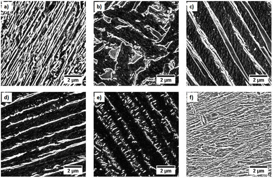
Figure 6.
Representative scanning electron microscope (SEM) images of the six microstructure classes found in the samples, after cropping to 350 × 350 px (equal to 9.70 × 9.70 µm): (a) pearlite, (b) granular bainite, (c) degenerated upper bainite, (d) upper bainite, (e) lower bainite, and (f) martensite. Etching was done using 2% Nital.
3.2. Microstructure Classification
All six microstructure classes found in the samples were considered for the classification task: pearlite (P), granular bainite (GB), degenerated upper bainite (DUB), upper bainite (UB), lower bainite (LB), and martensite (M). Classification was performed using only Haralick parameters, only local binary pattern (single-scale and multi-scale), as well as a combination of both. Results are presented by confusion matrices (CM) in which overall accuracy and F1 score as well as class recalls and precisions and F1 scores for each class are shown. The accuracy is the ratio of correctly predicted examples by the total examples. Recall is defined as the ratio of true positives by the sum of true positives plus false negatives while precision is the ratio of true positives by the sum of true positives plus false positives. F1 score is a function of recall and precision which can be used if a balance between these two metric is wanted or when the data set is unbalanced which is the case in this study because of the dominance of degenerated upper bainite structures in the reference samples. F1 score is the product of precision and recall times two, divided by the sum of precision and recall. Accordingly, F1 score is calculated for each class. Overall F1 score is the mean value of F1 scores of each class.
3.3. Classification Using Haralick Parameters
Table 3 shows the CM for the classification using Haralick parameters. As there are some differences in class recalls and precisions, the F1 score is also added for each class. Accuracies are high for pearlite, granular and degenerated upper bainite and martensite, but lower for upper and lower bainite.
Table 3.
Confusion matrix for the classification using Haralick textural parameters with a quadratic kernel support vector machine (SVM).
3.4. Classification Using Local Binary Pattern
3.4.1. Single-Scale Local Binary Pattern
Table 4 shows the CMs for the four different settings of the single-scale LBP. The 1/8 LBP does not yield particularly good classification results, especially for upper bainite there are several misclassifications. The overall accuracies of the other three single-scale LBP are good and comparable. However, precisions and recalls for the separate classes vary strongly.
Table 4.
Confusion matrices for the classification using single-scale local binary pattern: (a) radius R = 1, number of neighbors N = 8 (1/8), (b) 2.4/8, (c) 4.2/16, and (d) 6.2/16.
3.4.2. Multi-Scale Local Binary Pattern
By combining the four different neighborhood parameters into one multi-scale LBP, the accuracy is significantly improved to 88.70%.
Table 5 Accuracies for separate classes, assessed by the F1 score, are now high for all six microstructure classes.
Table 5.
Confusion matrix for the classification using multi-scale local binary pattern with a quadratic kernel SVM.
3.5. Classification Using a Combination of Haralick Parameters and Local Binary Pattern
As the Haralick classification gives a higher accuracy for granular bainite than the LBP multi-scale classification but is lower for other microstructure classes, both features are combined in the hope of improving the classification result. Table 6 shows the confusion matrix. The accuracy is slightly improved to 90.60%.
Table 6.
Confusion matrix for the classification using a combination of Haralick parameters and multi-scale local binary pattern with a quadratic kernel SVM, without feature selection.
Combining Haralick parameters and multiclass LBP gives a big set of features (64). For a better generalization, correlative features are removed. After doing this, only 31 features were kept. By this, the classification result could even be slightly improved to 91.80% (Table 7).
Table 7.
Confusion matrix for the classification using a combination of Haralick parameters and multi-scale local binary pattern with a quadratic kernel SVM, after removing correlative features.
4. Discussion
The work of Azimi et al. [13] can be viewed as the state of the art in microstructure classification of low-carbon steels. The only drawback of their approach is that Deep Learning is inherently difficult to interpret. Gola et al. [12] worked with the same data set, but used morphological and textural parameters in a combination with a support vector machine for classification. This approach can be better linked to the metallurgical processes and material properties. Gola et al. showed that both morphological parameters of the investigated objects and morphological and textural parameters of the substructure of these objects are important for their classification, as all three parameter groups were represented almost equally after feature selection. In continuing this approach and expanding it to bainitic structures the focus is now on using textural parameters as they showed to be very promising.
4.1. Classification Results
Table 8 summarizes the classification results of all the used features. With the confusion matrices showed earlier, this clearly shows that features calculated from the image texture can be used to successfully distinguish complex bainitic microstructures. Best results, an excellent classification accuracy of 91.80%, were obtained by combining Haralick parameters and a multi-scale LBP, followed by a feature selection. Picture IDs allow to trace back from classification result to textural parameters to the original microstructure images, which permits to asses which microstructure images where correctly or wrongly classified. Figure 7 shows examples for correctly classified images for all six microstructure classes.
Table 8.
Overview of classification results for the different features that were used to classify.
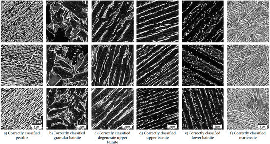
Figure 7.
Examples of correctly classified images for each microstructure class.
The main application option for this suggested classification approach based on reference samples would be the training of a model which could then be used as a pre-classification respectively labeling for other classification tasks. For a task of classifying complex steel microstructures, i.e., bainite, the assignment of the ground truth can be quite objective because bainitic phase constituents are often small or inhomogeneous, and there is often no consensus among human experts in labeling and classifying bainitic structures. This makes it difficult to extract ground truth parameters from these regions in an objective and statistically secured way. By incorporating these reference microstructures, the ground-truth assignment will be much more objective.
Considering the amount of analyzed pictures and the variety of structures even in one microstructure class which cause a broad distribution of values, it is difficult to draw definite conclusions about how the microstructures correlate with the calculated textural parameters and the classification result. Actually, this is one reason why machine learning methods are needed to be able to classify these microstructures. But still, some indications can be found when comparing textural parameters and microstructures. Figure 8 shows four Haralick parameters, i.e., the mean values of contrast, correlation and energy as well as the amplitude of correlation. Black dots represent the single values of every single image, red dots assign the mean value of all images. Contrast is a measure of the local variations in an image [21]. Correlation is a measure of how correlated a pixel is to its neighbor over the whole image, i.e., the joint probability occurrence of the specified pixel pairs [29]. Energy measures the uniformity of the gray level distribution in an image [30]. Few entries in the GLCM that have high probability, lead to a high energy value. Homogeneity measures the closeness of the distribution of elements in the GLCM to the GLCM diagonal [29], i.e., only entries close to the diagonal have a high impact on the value of the homogeneity.
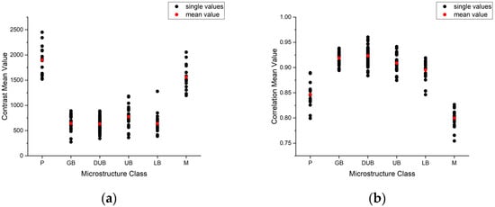
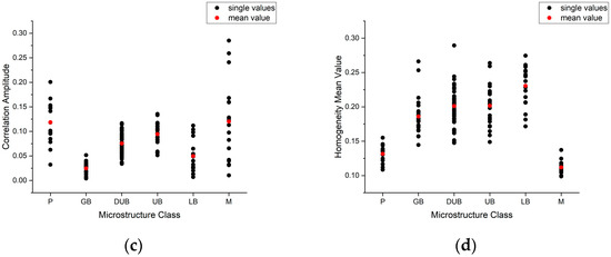
Figure 8.
Haralick Parameters: (a) contrast mean value, (b) correlation mean value, (c) correlation amplitude, and (d) homogeneity mean value.
Looking at the mean value of contrast, values for pearlite and martensite are significantly higher than for the bainitic structures, so that even when considering the scattering of the data, the bainitic classes could almost be separated from pearlite and martensite by setting a threshold. Low contrast values mean fewer local variations in the image. For the bainitic structures, there is always the dark bainitic ferrite as a “background”. This dark background, which has only few local variations, represents a considerable part of the image, explaining the lower overall contrast values for the bainitic structures. In a similar way, the higher correlation values for bainitic structures can be explained. Because of the “background” more “dark pixel pairs” occur, leading to higher correlation values. Pearlite tends to have higher contrast and correlation values compared to martensite. This could be explained by the ferrite-cementite transitions that occur in the pearlitic microstructure because of the topography contrast, caused by using Everhart-Thornley Detector in the SEM. Regarding bainitic structures, not much tendencies can be seen because the scattering can overshadow the trend. However, for the amplitude value of correlation, granular and lower bainite tend to have lower values than upper and degenerated upper bainite. In general, amplitude values will be higher for structures with certain preferential directions and lower for statistically distributed structures. While upper and degenerated upper bainite have a pronounced lath structure of the carbon-rich second phase, the distribution of this second phase is more statistically distributed in granular and lower bainite, causing lower amplitude value for correlation. Lower bainite still has a preferential direction (60° arrangement of intra-lath precipitates), however it is less pronounced than in upper and degenerated upper bainite. Taking this into account, pearlite should show higher amplitude values than martensite. However, their values partly overlap. The reason for this is that not all pearlitic pictures have straight continuous cementite laths but are already a bit degenerated with less preferential orientation.
Local binary pattern are good at capturing small and fine details of images [31], e.g., edges, corners, spots, etc. One disadvantage is that they can have problems to distinguish textures that have the same small structures but differ in their large structures. LBPs used in this work are rotation invariant uniform LBP. By using uniform LBP, the length of the histogram, i.e., the feature vector can be reduced and the performance of classifiers using these LBP features can be improved [22,32].
In a try to correlate LBP features, the microstructures and the classification results, Figure 9 shows the LBP 1/8 for the six microstructure images from Figure 6, which are representative for the six classes and show clear differences. Bainitic structures show higher values for bin 0, which represents bright spots [22], than pearlite and martensite, correctly capturing the arrangement of bright carbon-rich second phase in a dark bainitic ferrite background of the bainitic structures, compared to the more uniform gray level distribution of pearlite and martensite. Bins 1–7, which correspond to different edges or corners of varying positive and negative curvature [22], partly show differences which is plausible, as the images also exhibit different kind of edges. However, several bins show only marginal differences, especially for bainitic structures, already indicating that this LBP could not provide enough discrimination for the classification of bainitic structures. Figure 10 shows the averaged histograms of the local binary pattern with R = 1 and N = 8 of all images for all six microstructure classes, which reached an accuracy of just 74.20%. For an easier visualization, histograms are averaged by calculating the mean value of the separate bins for every analyzed image. This allows for some indications how the LBPs, the microstructures and the classification results correlate. Pearlite and martensite show quite different histograms while the histograms of the four bainitic structures are similar. For a better illustration and a closer look at differences, some histogram bins (bins 1, 5, 6, and 9) are separately shown in Figure 11a. Error bars for the standard deviation are added to indicate the scattering of all the images. Pearlite and martensite can be distinguished quite well, also when considering the scattering. Contrary, values for bainite are comparable most of the time, giving a hint that a differentiation of bainitic structures with these features will be difficult. Looking at the confusion matrix for this LBP in Table 4, there are strong variations between the recalls and precisions of the individual classes. Indeed, F1 scores for pearlite and martensite are high and lower for bainitic structures which fits the differences that are indicated by the histograms. Also, for the R = 2.4 and N = 8 as well as the R = 4.2 and N = 16 LBP, the results for pearlite and martensite are good and clearly better than the results for the bainitic structures. When looking at the representative SEM images for all classes, pearlite and martensite are the “densest” structures compared to bainitic structures, which have more “background” (the dark bainitic ferrite). So basically, the representative area to capture to relevant features of a microstructure is smaller for pearlite and martensite and bigger for the bainitic structures. That’s why these three single-scale LBP achieve better results for pearlite and martensite.
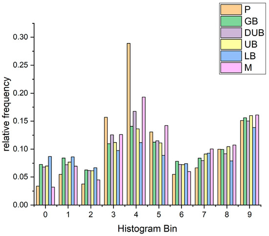
Figure 9.
LBP 1/8 for representative images from Figure 5 for all six microstructure classes, showing differences in the separate bins of the histogram.
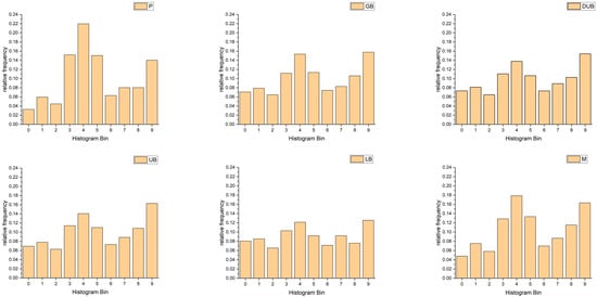
Figure 10.
Averaged histograms of LBP with R = 1 and N = 8 of all images for all six microstructure classes. Averaging performed by calculating the mean value of the separate bins for every analyzed image.
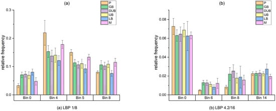
Figure 11.
Individual bins of the LBP 1/8 (a) and LBP4.2/16 (b) histograms for all six microstructure classes, for a better illustration of differences. Error bars are standard deviations to indicate the scattering of all analyzed images.
The R = 4.2 and N = 16 LBP gave the best results for the single-scale LBP with 83.60% accuracy. Figure 12 shows the averaged histograms for all six microstructure classes. Again, for an easier visualization, histograms are averaged by calculating the mean value of the separate bins for every analyzed image. Also, some histogram bins (bins 1, 7, 9, and 15) are separately shown in Figure 11b for a closer look at differences. Although there is always overlap because of the scattering, a tendency of clearer differences in the bainitic classes compared to the LBP 1/8 can be recognized, explaining the better classification result with this LBP.
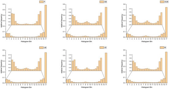
Figure 12.
Averaged histograms of LBP with R = 4.2 and N = 16 of all images for all six microstructure classes. Averaging performed by calculating the mean value of the separate bins for every analyzed image. Bins 0–16 are also shown enlarged.
Looking at all four single-scale LBP, the overall accuracies are mediocre to good (maximum accuracy of 83.60% for LBP 4.2/16) and there are usually strong variations between the recalls and precisions of the individual classes. This clearly shows that by considering only a single scale for the LBP, not all relevant features of the six different microstructures can be captured. By combining the four scales from the single-scale LBP into one multi-scale LBP the overall accuracy improves to a very good 88.70%. Accuracies for separate classes, assessed by the F1 score, are high for all classes.
As LBP features capture small and fine details of an image and Haralick parameters recognize image features on a bit bigger scale, it seems reasonable to try to combine Haralick and LBP features. Furthermore, Haralick classification gives a higher accuracy for granular bainite than the LBP multi-scale classification, but is lower for other microstructure classes, so they could perhaps complement one another. Indeed, by combining those features, the overall classification accuracy gets improved to 90.60%. Because the combination of these parameters gives a big set of features (64), correlative features are removed for a better generalization. Only 31 features were kept, and by this, the classification result could again be slightly improved to 91.80%.
Figure 13 gives some examples of misclassified microstructure images. With Picture IDs, textural parameters and the original microstructure images can be traced back from the classification results. This allows to check which feature in the microstructure image could have caused a misclassification. Figure 13a shows a martensitic microstructure that was classified as pearlite. Comparing it with a correctly classified martensitic image (Figure 13b) the structure of the misclassified martensite is more ordered and less chaotic and thereby looking similar to a pearlitic microstructure, as shown in Figure 13c. In Figure 13d a lower bainite image that was misclassified as upper bainite is shown. The reason is probably that the lower bainite also exhibits some cementite precipitation on the lath boundaries in addition to the intra-lath cementite precipitation. Figure 13e shows upper bainite that was wrongly classified as degenerated upper bainite. This could be explained by the fact that not all precipitation on the lath boundaries are straight and slender and that there are also some cementite aggregates giving it a bit of a degenerated structure. These examples show the difficulty in bainite classification as one bainite subclass can also exhibit some features that are more associated with other subclasses, making the ground truth assignment challenging even though reference samples were used in this work. In principle, such images could be left out for the classification which would improve the classification result. However, it is a goal to cover all ranges of bainitic microstructures and because multi-phase steels or industrial samples will also exhibit mixed structures it was decided to keep these images in the data set.
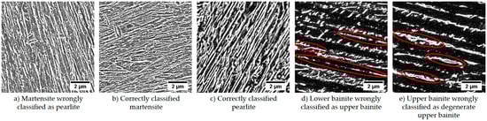
Figure 13.
Examples of misclassified pictures: (a) wrongly martensite showing a regular lath structure compared to the more irregular laths of correctly classified martensite (b) and similar to pearlite (c), (d) lower bainite with some slender cementite precipitation on the lath boundaries (red), similar to upper bainite, and (e) upper bainite with some cementite aggregates, similar to degenerated upper bainite.
4.2. Extensions to the Classification Approach
When looking at the CM in Table 7, 9 of the 13 wrongly classified images come from mix-ups of lower, upper, and degenerated upper bainite. These three bainite classes are the most similar microstructures because they all exhibit a lath-like structure. One way to improve the classification result could be to combine these three bainite types into one class: lath-like bainite. After classifying pearlite, granular bainite, lath-like bainite, and martensite, morphological parameters could be used to further separate the lath-like bainite into the original lower, upper, and degenerated upper bainite because all three types have different morphological characteristics. Lower bainite usually has many small cementite precipitates in the ferrite laths, upper bainite has longer cementite particles whereas the carbon-rich phase in degenerated upper bainite is wider than the cementite of upper bainite.
The images analyzed in this work were squared images, cut in a uniform way from a bigger image. Usually regions of a specific microstructure are not squared, but have some arbitrary, irregular shape. In future work, the suggested classification approach could be applied to real microstructure objects instead of squared images.
This work already covered a wide variety of bainitic microstructures. However, for granular bainite, more variations of the carbon-rich second phase exist. In this work, this carbon-rich second phase was mainly composed of MA particles with some debris of cementite. Zajac et al. [7] also define degenerated pearlite or incomplete transformation products as carbon-rich second phases. In future work, these different variations in granular bainite could also be included in the classification task. Furthermore, self-tempered martensite could also be added. The production of isothermally transformed samples could also be tried. If the goal would be a universal bainite classification of all kinds of bainitic steels, more reference samples could be produced to build a more robust model.
From the machine learning perspective, the SVM could be further tuned and additional feature selection could be tried. Furthermore, by using data augmentation, especially for the microstructure classes that are less represented, in order to get better balanced classes, the model could perhaps be improved.
Although using these reference samples gives more objectivity, there is still some subjectivity in assigning the classes for the ground truth. First, when using only SEM images for labeling some uncertainty will always remain. This could be improved by adding correlative data from TEM or EBSD analysis. However, the time required and the limited areas that can be measured restrict the practical use. Second, the choice of the classification scheme is already subjective. In this work, the scheme suggested by Zajac [7] was used, however there are many more schemes available in the literature, as discussed in the introduction. When choosing a different classification scheme for these reference samples, the classification result will also be different. To overcome this problem and make the classification even more objective, future work will incorporate unsupervised learning techniques. Contrary to the supervised learning approach used in this work, no ground truth is given for unsupervised learning. These techniques can be used to cluster data or raw images by finding similarities. For data clustering, different algorithms like k-means, k-medoids, or hierarchical clustering are available. The raw images can also be clustered by using a pre-trained neural network as a feature extractor, followed by a clustering of these features with a clustering algorithm. Such an approach is presented by Kitahara et al. [33].
5. Conclusions
- Microstructures considered in the classification are pearlite, granular bainite, degenerated upper bainite, upper bainite, lower bainite, and martensite, with bainite types according to the scheme suggested by Zajac [7]. An excellent classification accuracy of 91.80% is reached, showing the feasibility of using textural features to distinguish bainitic microstructures.
- The images used in this work come from specifically produced samples, by using a quenching dilatometer, in order to get reference bainitic structures. This allows a more objective ground truth assignment for the classification which is, when dealing with complex microstructures like bainite, otherwise it is a challenging task with a big subjective component.
- In continuing this approach, these reference samples and the classification model based on them can be used as a more objective ground truth assignment for other tasks of classifying complex steel microstructures, i.e., bainite, especially when analyzing multi-phase industrial steel grades.
- In future work, unsupervised learning techniques will be implemented to eliminate the subjective component of choosing a classification scheme, which will make the ground truth assignment again more objective.
Supplementary Materials
The following are available online at https://www.mdpi.com/2075-4701/10/5/630/s1, Supplementary materials include representative SEM micrographs of each sample before cropping, to give an overview of the overall microstructures.
Author Contributions
Conceptualization, M.M. and D.B.; Formal analysis, M.M. and L.U.; Investigation, M.M.; Methodology, M.M. and L.U.; Supervision, D.B., T.S., and F.M.; Visualization, M.M.; Writing—original draft, M.M.; Writing—review & editing, M.M., D.B., T.S., and F.M. All authors have read and agreed to the published version of the manuscript.
Funding
This research received no external funding.
Acknowledgments
The authors thank steel manufacturer AG der Dillinger Hüttenwerke for providing the sample material and TA Instruments for the production of the reference samples by using DIL 805 A/D quenching dilatometer. Furthermore, the authors thank Johannes Webel who programmed a MATLAB script for automatic calculation of Haralick textural features. The authors acknowledge Saarland University within the funding program Open Access Publishing.
Conflicts of Interest
The authors declare no conflict of interest.
References
- Bhadeshia, H.K.D.H. Bainite in Steels, 3rd ed.; Maney Publishing: Leeds, UK, 2015. [Google Scholar]
- Ohmori, Y.; Ohtani, H.; Kunitake, T. The Bainite in Low Carbon Low Alloy High Strength Steels. Tetsu-to-Hagane 1971, 57, 1690–1705. [Google Scholar] [CrossRef]
- Bramfitt, B.L.; Speer, J.G. A perspective on the morphology of bainite. Metall. Trans. A 1990, 21, 817–829. [Google Scholar] [CrossRef]
- Lotter, U.; Hougardy, H.P. Kennzeichnung des Gefüges Bainit. Prakt. Metallogr. 1992, 29, 151–157. [Google Scholar]
- Krauss, G.; Thompson, S.W. Ferritic Microstructures in Continuously Cooled Low- and Ultralow-carbon Steels. ISIJ Int. 1995, 35, 937–945. [Google Scholar] [CrossRef]
- Fischer, M.D. Quantitative Analyse feinkörniger, komplexer und mehrphasiger Mikrostrukturen. Ph.D. Thesis, Rheinisch-Westfälische Technische Hochschule Aachen, Aachen, Germany, 22 December 2015. [Google Scholar]
- Zajac, S.; Schwinn, V.; Tacke, K.H. Characterisation and Quantification of Complex Bainitic Microstructures in High and Ultra-High Strength Linepipe Steels. Mater. Sci. Forum. 2005, 500–501, 387–394. [Google Scholar] [CrossRef]
- Araki, T. Atlas for Bainitic Microstructures; ISIJ Bainite Committee: Tokyo, Japan, 1992. [Google Scholar]
- Gerdemann, F.L.H.; Bleck, W. Bainite in medium carbon steels; Shaker Verlag GmbH: Düren, Germany, 2010. [Google Scholar]
- Aarnts, M.P.; Rijkenberg, R.A.; Twisk, F.A.; Wilcox, D.; Zuijderwijk, M.J.; Arlazarov, A.; Barbier, D.; Germain, L.; Gouné, M.; Hazotte, A.; et al. Microstructural quantification of multi-phase steels (Micro-quant), European Commission. Res. Fund for Coal Steel 2011. [Google Scholar] [CrossRef]
- Song, W. Characterization and Simulation of BAINITE Transformation in High Carbon Bearing Steel 100Cr6; RWTH Aachen Aachen: Aachen, Germany, 2014. [Google Scholar]
- Gola, J.; Webel, J.; Britz, D.; Guitar, A.; Staudt, T.; Winter, M.; Mücklich, F. Objective microstructure classification by support vector machine (SVM) using a combination of morphological parameters and textural features for low carbon steels. Comput. Mater. Sci. 2019, 160, 186–196. [Google Scholar] [CrossRef]
- Azimi, S.M.; Britz, D.; Engstler, M.; Fritz, M.; Mücklich, F. Advanced steel microstructural classification by deep learning methods. Sci. Rep. 2018, 8, 1–14. [Google Scholar] [CrossRef]
- Zajac, S.; Komenda, J.; Morris, P.; Dierickx, P.; Matera, S.; Diaz, F.P. Quantitative Structure-Property Relationships for Complex Bainitic Microstructures. 2005. Available online: https://publications.europa.eu/en/publication-detail/-/publication/22f902b8-37e3-4fa1-86fe-5876e4974329 (accessed on 29 April 2020).
- Tsutsui, K.; Terasaki, H.; Maemura, T.; Hayashi, K.; Moriguchi, K.; Morito, S. Microstructural diagram for steel based on crystallography with machine learning. Comput. Mater. Sci. 2019, 159, 403–411. [Google Scholar] [CrossRef]
- Komenda, J. Automatic recognition of complex microstructures using the Image Classifier. Mater. Charact. 2001, 46, 87–92. [Google Scholar] [CrossRef]
- Miyama, E.; Voit, C.; Pohl, M. Zementitnachweis zur Unterscheidung von Bainitstufen in modernen, niedriglegierten Mehrphasenstählen. Prakt. Metallogr. 2011, 48, 261–272. [Google Scholar] [CrossRef]
- Banerjee, S.; Datta, S.; Paul, B.; Saha, S.K. Segmentation of three phase micrograph: An automated approach. Proc. CUBE Int. Inf. Technol. Conf. ACM 2012, 1–4. [Google Scholar] [CrossRef]
- Paul, A.; Gangopadhyay, A.; Chintha, A.R.; Mukherjee, D.P.; Das, P.; Kundu, S. Calculation of phase fraction in steel microstructure images using random forest classifier. IET Image Process. 2018, 12, 1370–1377. [Google Scholar] [CrossRef]
- Shapiro, L. Computer Vision and Image Processing; Academic Press: San Diego, CA, USA, 1992. [Google Scholar]
- Haralick, R.; Shanmugan, K.; Dinstein, I. Textural features for image classification. IEEE Trans. Syst. Man Cybern. 1973, 3, 610–621. [Google Scholar] [CrossRef]
- Ojala, T.; Pietikäinen, M.; Mäenpää, T. Multiresolution gray-scale and rotation invariant texture classification with local binary patterns. IEEE Trans. Pattern Anal. Mach. Intell. 2002, 24, 971–987. [Google Scholar] [CrossRef]
- Webel, J.; Gola, J.; Britz, D.; Mücklich, F. A new analysis approach based on Haralick texture features for the characterization of microstructure on the example of low-alloy steels. Mater. Charact. 2018, 144, 584–596. [Google Scholar] [CrossRef]
- Gupta, S.; Sarkar, J.; Kundu, M.; Bandyopadhyay, N.R.; Ganguly, S. Automatic recognition of SEM microstructure and phases of steel using LBP and random decision forest operator. Measurement 2020, 151. [Google Scholar] [CrossRef]
- Wibmer, A.; Hricak, H.; Gondo, T.; Matsumoto, K.; Veeraraghavan, H.; Fehr, D.; Zheng, J.; Goldman, D.; Moskowitz, C.; Fine, S.W.; et al. Haralick texture analysis of prostate MRI: Utility for differentiating non-cancerous prostate from prostate cancer and differentiating prostate cancers with different Gleason scores. Eur. Radiol. 2015, 25, 2840–2850. [Google Scholar] [CrossRef]
- Mäenpää, T.; Pietikäinen, M. Multi-scale binary patterns for texture analysis. Lect. Notes Comput. Sci. 2003, 2749, 885–892. [Google Scholar] [CrossRef]
- Gola, J.; Britz, D.; Staudt, T.; Winter, M.; Schneider, A.S.; Ludovici, M.; Mücklich, F. Advanced microstructure classification by data mining methods. Comput. Mater. Sci. 2018, 148, 324–335. [Google Scholar] [CrossRef]
- Gupta, C.; Dey, G.K.; Chakravartty, J.K.; Srivastav, D.; Banerjee, S. A study of bainite transformation in a new CrMoV steel under continuous cooling conditions. Scr. Mater. 2005, 53, 559–564. [Google Scholar] [CrossRef]
- Texture Analysis Using the Gray-Level Co-Occurrence Matrix (GLCM) - MATLAB & Simulink - MathWorks Deutschland, (n.d.). Available online: https://de.mathworks.com/help/images/texture-analysis-using-the-gray-level-co-occurrence-matrix-glcm.html (accessed on 13 March 2020).
- Dutta, S.; Barat, K.; Das, A.; Das, S.K.; Shukla, A.K.; Roy, H. Characterization of micrographs and fractographs of Cu-strengthened HSLA steel using image texture analysis. Measurement 2014, 47, 130–144. [Google Scholar] [CrossRef]
- Pietikäinen, M.; Zhao, G. Two decades of local binary patterns: A survey. In Advances in Independent Component Analysis and Learning Machines; Academic Press: Cambridge, MA, USA, 2015; pp. 175–210. [Google Scholar] [CrossRef]
- Lahdenoja, O.; Poikonen, J.; Laiho, M. Towards Understanding the Formation of Uniform Local Binary Patterns. ISRN Mach. Vis. 2013, 2013, 1–20. [Google Scholar] [CrossRef]
- Kitahara, A.R.; Holm, E.A. Microstructure Cluster Analysis with Transfer Learning and Unsupervised Learning. Integr. Mater. Manuf. Innov. 2018, 7, 148–156. [Google Scholar] [CrossRef]
© 2020 by the authors. Licensee MDPI, Basel, Switzerland. This article is an open access article distributed under the terms and conditions of the Creative Commons Attribution (CC BY) license (http://creativecommons.org/licenses/by/4.0/).