Article

Calibration of Advanced Yield Criteria Using Uniaxial and Heterogeneous Tensile Test Data

Faculty of Mechanical Engineering, University of Ljubljana, Aškerčeva, 61000 Ljubljana, Slovenia
*
Author to whom correspondence should be addressed.
Metals 2020, 10(4), 542; https://doi.org/10.3390/met10040542
Submission received: 6 April 2020 / Revised: 19 April 2020 / Accepted: 20 April 2020 / Published: 22 April 2020
(This article belongs to the Special Issue Challenges and Achievements in Metal Forming)

Abstract

:
Conventionally, plastic anisotropy is calibrated by using standard uniaxial tensile and biaxial test results. Alternatively, heterogeneous strain field specimens in combination with full-field measurements can be used for this purpose. As reported by the literature, such an approach reduces the number of required tests enormously, but it is challenging to obtain reliable results. This paper presents an alternative methodology, which represents a compromise between the conventional and heterogeneous strain field calibration technique. The idea of the method is to use simple tests, which can be conducted on the uniaxial testing machine, and to avoid the use of advanced measuring equipment. The procedure is accomplished by conducting standard tensile tests, which are simple and reliable, and by a novel heterogeneous strain field tensile test, to calibrate the biaxial stress state. Moreover, only two of the parameters required for full characterisation need to be inversely identified from the test response; the other parameters are directly determined from the uniaxial tensile test results. This way, a dimension of optimization space is reduced substantially, which increases the robustness and effectiveness of the optimization algorithm.

1. Introduction

In sheet metal forming processes, mechanical behaviour usually depends on the extent of plastic anisotropy. To accurately predict the behaviour, advanced yield criteria have been introduced [1]. The accuracy of the predictions depends on the flexibility of the yield function, which is correlated to a set of parameters that have to be calibrated against experimental data. Following a standard identification procedure [2], this is achieved by utilizing the inputs of three uniaxial tensile tests [3], i.e., one in the parallel direction (0°), one in the transverse direction (90°) and one in the diagonal direction (45°) measured from the rolling direction. During the testing procedure, normalized flow stresses and width-to-thickness strain ratio (R-values) [4] are measured. Additionally, to characterize biaxial flow stress and biaxial R-value, a bulge test [5], through-thickness disk compression test [6,7] or a cruciform specimen test [8,9,10] needs to be conducted. However, such intricate experimental procedures require specific testing equipment, which may not always be available in industrial labs.
Recently, an attractive alternative has been proposed by a merger of full-field measurement techniques like the Digital Image Correlation (DIC) and inverse identification methods, even for advanced material models [11] and a large number of material parameters. The approach relies upon conducting a test with a heterogeneous strain–stress field, from which a larger quantity of different experimental data can be measured [12]. This way, the number of required tests for full anisotropy calibration can be reduced to a single test. Within this proposition, two research areas developed spontaneously: the development of heterogeneous strain–stress field test specimens and the development of inverse identification methods.
The key feature of the former is the design of a testing procedure that enables reliable parameter identification, which is achieved by the increased heterogeneity of the resulting strain–stress state. In other words, the design strives for the maximum number of possible states that alter within the test sample. Moreover, a strong correlation between the measured strain state and sought parameters should be ensured.
As for the latter—with the full-field experimental techniques available, associated identification methods have also developed. Among them, the finite element model updating method (FEMU) [13,14], constitutive equation gap method (CEGM) [15], virtual fields method (VFM) [16,17], equilibrium gap method (EGM) [18] and others, e.g., [19,20], are well established. A complete overview of the methods can be found in Avril et al. [21].
There have been many attempts to undertake the concept of full-field identification of anisotropy parameters from only a single test. Meuwissen et al. [22] made an early attempt to identify the Hill48 model parameters by utilizing a heterogeneous strain field specimen for use on a uniaxial tensile-testing machine. In their study, they employed the FEMU method to identify anisotropy and hardening behaviour, and they reported that the Hill48 model provides a better fit to experimental data in comparison to the isotropic von Mises model. Their specimen served as the basis for later test improvements to achieve higher plastic strains. In particular, Haddadi and Belhabib [23] enhanced the heterogeneous strain state tensile test to achieve improved strain heterogeneity, strain-path variety and sensitivity to hardening parameters. Moreover, Robert et al. [24] compared the Haddadi and Meuwissen specimen geometries and concluded that specimen geometry has a crucial influence on the identified parameters. According to the study, Haddadi’s geometry is more suitable, owing to a more uniform heterogeneous strain distribution. By contrast, Meuwissen’s geometry yields high strain gradients that are spatially very localized.
A similar test to that of Haddadi and Belhabib [23] was conducted by Güner et al. [25] for YLD2000-2d model calibration. In the study, they found that the employed specimen is insufficient for biaxial stress state calibration and that additional biaxial test is needed. The reason for such an approach originates from the specimen’s shape. The shape is similar to that used in a uniaxial tensile test, with a neck introduced in the middle section. Hence, during loading, only stress states between uniaxial tension and plane strain emerge. This impediment was also exposed by Kim et al. [26]. As reported, they were unable to identify anisotropy and hardening parameters from the notched specimen since the specimen does not provide sufficient information for each parameter. Therefore, the geometry alone is unsuited to the simultaneous identification of all anisotropy parameters. Based on the finding, they conducted tests using three specimen designs: a notched specimen with two diametrically arranged holes, a butterfly-shaped tensile specimen with four holes and a Σ-shaped specimen. By analysing the stress state heterogeneity, they showed that the Σ-shaped specimen has the highest degree of heterogeneity and that all stress states, from shear to biaxial tension, are present. They exposed that high strain field magnitudes could result in poor identification results if they are located where it is difficult to obtain reliable measurements (i.e., free edges).
The objective of the design is to develop a heterogeneous strain field specimen whose shape clearly expresses the information relevant to the sought parameters. However, this is not sufficient for an identification procedure to be effective. In particular, the effectiveness also depends on the non-linearity of the material model and the number of sought parameters. As exposed by Kowalewski and Gajewski [27], this is a significant disadvantage of FEMU-based identification schemes, where the number of required iterations to reach convergence can be high. Convergence is affected by the optimization algorithm being employed. Furthermore, the algorithms do not guarantee that the optimum parameters are always found for different initial values [28,29].
To address these drawbacks, an alternative VFM was developed. Its main advantage is that it does not need to use finite element calculations. As reported by Martins et al. [30], the weakness of the method is the choice of virtual fields, especially in non-linear cases.
Advantageous for this method is that it incorporates complete strain field information [31], while on the other hand, full-field experimental data over an entire domain is required in the identification process [30]. If the material does not follow the assumed plasticity model, the method returns the parameters that best fit the experimental behaviour. However, Rossi et al. [32] exposed that the higher the heterogeneity, the more difficult it is to find a good compromise. In that case, a single test is no longer sufficient to identify the parameters. In addition to the Hill48 model, they also identified the parameters of the YLD2000-2d model, but validation was beyond their scope.
Recently, Lattanzi et al. [33] introduced a novel VFM-based inverse identification methodology for large-strain applications to identify YLD2000-2D yield function parameters by using a deep-notched tensile specimen at three different orientations. The values of the parameters lead to a reasonable reproduction of the anisotropy, but the experimental effort required for the calibration of such an advanced material model was reduced to three tests. As exposed, one heterogeneous strain field test is insufficient for complete anisotropy calibration.
This paper presents an alternative methodology, which represents a compromise between the conventional anisotropy calibration procedure as described in [34] and full-field measurement-based approaches, as outlined above. Conventionally, the uniaxial yield stress Y 0 , Y 90 ,   Y 45 , the biaxial yield stress Y B and corresponding R-values R 0 ,     R 90 ,     R 45 and R B are first expressed with the model’s parameters. Secondly, these expressions are equalised with corresponding experimental values, and finally, the system of equations is solved. As mentioned, such an approach requires a bulge, disk compression or cruciform specimen test, which demands special testing equipment. Alternatively, to avoid intricate biaxial testing, a heterogeneous strain field tensile specimen can be employed, but this approach usually forgoes the use of simple and reliable standard uniaxial tensile tests. Moreover, the large number of parameters hinders the identification procedure, owing to the high dimensionality of parametric hyperspace.
Herein we present an identification procedure for the calibration of the YLD2000-2d model. The method combines a heterogeneous strain field tensile test and a standard uniaxial tensile test but avoids both the use of special equipment needed for biaxial testing and a large number of identification parameters. Moreover, a FEMU-based inverse identification procedure is applied for the identification of two parameters, whereas other parameters are calculated from the standard uniaxial tests data directly.
Importantly, to avoid a large number of parameters in the identification procedure, and to simplify the identification procedure, the parameters of the employed YLD2000-2d model α 1 ,   α 2 , , α 8 are firstly expressed as parameters with physical meaning Y 0 ,     Y 90 ,   Y 45 ,   Y B ,   R 0 ,     R 90 ,   R 45 ,   by using a conversion procedure as described in [35]. As exposed by Marek et al. [36,37], the lack of physical explanation has a significant impact on the identification procedure outcome, which is driven by the compound action of all parameters.
Based on this concept, the parameters α 1 ,   α 2 , , α 8 are first expressed with normalized flow stresses Y 0 ,     Y 90 ,   Y 45 ,   Y B and R-ratios, R 0 ,     R 90 ,   R 45 and R B . Moreover, with the uniaxial testing machine being available, it is reasonable to determine six out of eight parameters by using uniaxial test data in three directions. The measured flow stresses Y 0 ,     Y 90 ,   Y 45 and width-to-thickness strain ratios R 0 ,     R 90 ,   R 45 can be used directly as the model inputs.
In such a way, we (i) take advantage of standard uniaxial tensile tests which are simple, accurate and easy to perform, and (ii) reduce the number of sought parameters from eight to two, namely, Y B and R B The latter results in a reduction of the dimensionality of the parametric hyperspace and simplify the FEMU procedure substantially. For the identification of parameters Y B and R B , we designed a heterogeneous strain field specimen for use on a uniaxial tensile machine. Thus, we avoided additional testing equipment. The geometry is designed to manifest a pronounced biaxial stress state at the centre of the heterogeneous strain field specimen. Finally, the parameters are identified by minimizing the discrepancy between measured and simulated strain fields at the centre of the test specimen. The identified parameters, and consequently the proposed methodology, are verified by conducting a standard bulge test according to ISO 16808 [5].

2. Materials and Methods

2.1. The YLD2000-2d Model

The proposed methodology is applied to the widely accepted YLD2000-2d plastic anisotropy model, which is briefly outlined below. For a detailed description, the reader is referred to the works of Barlat et al. [6,34,35].
The anisotropic yield function of the model is defined by two linear transformations of the deviatoric part of the Cauchy stress tensor s . The yield function reads:
Φ s , Y = X 1 X 2 a + 2 X 1 + X 2 a + 2 X 2 + X 1 a = 2 Y a ,
where X 1 , X 2 , X 1 and X 2 are the principal values of two transformed stress deviator tensors X and X , defined by linear transformations X = C . s = C . T . σ = L . σ and X = C . s = C . T . σ = L . σ . The parameter a controls the curvature of the yield surface and usually depends on the crystal structure of the material, whereas the parameter Y presents the reference flow stress, dependent on the amount of accumulated equivalent plastic strain.
When considering a planar anisotropy, the transformation of the stress state σ yields only 10 nonzero coefficients in L and L , which are related to 8 independent parameters α 1 , α 2 , , α 8 :
L 11 L 12 L 21 L 22 L 66 = 1 3 2 0 0 1 0 0 0 1 0 0 2 0 0 0 3 α 1 α 2 α 7 ,   L 11 L 12 L 21 L 22 L 66 = 1 9 2 2 8 2 0 1 4 4 4 0 4 4 4 1 0 2 8 2 2 0 0 0 0 0 9 α 3 α 4 α 5 α 6 α 8 .
Conventionally, the parameters α 1 , α 2 , , α 8 are calibrated from the uniaxial test in three directions and the results of one biaxial test.

2.2. Conversion Between the Normalized Flow Stresses, R-Values and α i Parameters

For the employed anisotropy model, the parameters α 1 , α 2 , , α 8 can be determined from the normalized uniaxial flow stresses Y 0 ,     Y 90 ,   Y 45 ,     Y B , and R-values R 0 ,     R 90 ,   R 45 ,   R B by solving the following set of nonlinear equations:
A 1 a + B 2 a + C 3 a = 2 3 Y 0 a ,
A 3 a + B 1 a + C 2 a = 2 3 Y 90 a ,
A 2 a + B 3 a + C 1 a = 2 3 Y B a ,
2 a V a / 2 + W 2 a + W 1 a = 2 12 Y 45 a ,
R 0 A 2 + A 3 A 1 A 1 a 2 + R 0 B 3 + B 1 B 2 B 2 a 2 + R 0 C 1 C 2 C 3 C 3 a 2 = 0 ,
R 90 A 2 + A 1 A 3 A 3 a 2 R 90 B 3 + B 2 B 1 B 1 a 2 + R 90 C 1 + C 3 C 2 C 2 a 2 = 0 ,
A 1 1 + R B A 2 A 2 a 2 + R B B 2 B 1 B 3 B 3 a 2 + R B C 3 + C 2 C 1 C 1 a 2 = 0 ,
C 1 B 3 2 + K C 1 + B 3 W 2 W 1 a 2 W 2 a 2 = K 2 3 a 2 / Y 45 a 1 + R 45 A 2 3 2 V a 2 1 ,
where A 1 = 2 α 1 + α 2 , A 2 = α 2 α 1 , A 3 = α 1 + 2 α 2 , B 1 = 4 α 4 α 3 ,   B 2 = 2 α 3 2 α 4 , B 3 = α 3 + 2 α 4 , C 1 = 2 α 5 + α 6 , C 2 = 2 α 5 2 α 6 , C 3 = 4 α 5 α 6 , K = C 1 B 3 2 + 6 α 8 2 , W 1 , 2 = C 1 + B 3 ± K and V = A 2 2 + 6 α 7 2 .
It should be emphasized that this is a conventional identification procedure followed by Barlat et al. in their work [34]. As reported, Equations (3)–(10) can be easily solved by the Newton–Raphson method in a few iterations.
By contrast, the values Y 0 ,     Y 90 ,   Y 45 ,     Y B and R 0 ,     R 90 ,   R 45 ,   R B can also be interpreted as the identification parameters, which are inserted in the above system of equations to evaluate α 1 ,   α 2 , , α 8 . Consequently, the values Y 0 ,     Y 90 ,   Y 45 and R 0 ,     R 90 ,   R 45 can be equated with corresponding values measured from the uniaxial tensile test, whereas the parameters Y B and R B can be determined from the nonhomogeneous strain field tensile test response.

2.3. Proposed Identification Methodology

The proposed method represents a compromise between the conventional calibration procedure and full-field strain measurement identification methods. The process can be described in the following steps:
  • The standard uniaxial tensile tests [3] are first carried out in three directions, i.e., one parallel (0°), one transverse (90°) and one in a diagonal (45°) direction to the rolling direction. The hardening behaviour, normalized yield stresses and R-values are calculated directly from these tests.
  • The developed heterogeneous strain field specimen is tested by using a uniaxial tensile testing machine. The tensile force and the strain field at the centre of the test specimen are measured during the test. The test specimen is presented in Section 2.4.
  • The parameters are identified using a FEMU procedure, where the simulated heterogeneous test response is compared to the measured one. More specifically, the calculated test response depends on the α 1 ,   α 2 , , α 8   values, determined by Y 0 ,     Y 90 ,   Y 45 ,   R 0 ,     R 90 ,   R 45 ,     Y B and R B . This means that Y 0 ,     Y 90 ,   Y 45 ,   R 0 ,     R 90 ,   R 45 ,     Y B and R B can be considered as optimization input parameters, and parameters related to the uniaxial tensile test data can be directly set equal to their experimental values from uniaxial tests, i.e., Y 0 = Y 0 e x p ,   Y 90 = Y 90 e x p , Y 45 = Y 45 e x p , R 0 = R 0 e x p ,   R 90 = R 90 e x p ,     R 45 = R 45 e x p , and excluded from optimization. This means that only two parameters, Y B and R B , are sought by an inverse identification algorithm utilizing a heterogeneous strain field tensile test response. In other words, with the supplementary values Y 0 e x p ,     Y 90 e x p ,   Y 45 e x p ,     R 0 e x p ,     R 90 e x p and R 45 e x p , an arbitrary set of parameters { Y B ,   R B } can be converted to α 1 ,   α 2 , , α 8   parameters, which are used in the YLD2000-2d model simulations. We can also interpret this procedure as a constrained optimization problem, where the parameters α 1 ,   α 2 , , α 8   are constrained by six experimental values from the uniaxial tensile tests. This means that the dimensionality of the parametric space reduces from eight to two.
The proposed methodology is schematically presented in Figure 1. The left box (a) presents the tests to be performed. The outputs of these tests are the normalized uniaxial stresses, the R-values and the strain fields measured from the heterogeneous test. Together with the initial guesses for { Y B , R B } = 1 , 1 , the experimental values of Y 0 e x p ,     Y 90 e x p ,   Y 45 e x p ,     R 0 e x p ,   R 90 e x p and R 45 e x p are inserted in the conversion algorithm (b), which yields YLD2000-2d parameters α 1 ,   α 2 , , α 8 (see Section 2.2). These parameters are delivered in the numerical simulation of the conducted heterogeneous test (c). The output of the numerical simulation is strain field response at the centre of the specimen (d), which is compared with the experimental data (e) during the minimization procedure (f). New values of { Y B , R B } are then returned to the conversion algorithm (b) and the procedure is repeated to minimize the discrepancy between measured and simulated responses.

2.4. Development of the Heterogeneous Strain Field Specimen

As proposed by the identification methodology, a heterogeneous test is used for Y B and R B identification, where strain field and tensile force are to be measured. From this viewpoint, several requirements for a specimen design arise. Primarily, a biaxial stress state should be pronounced at the strain measurement locations and these locations should not be close to free edges, where it is difficult to obtain good experimental DIC measurements. Free-edge strain measurements are also affected by the edge roughness and manufacturing tolerances. Moreover, any stress concentrations or high strain gradients at measuring locations are not desired and should be avoided. This means that a pronounced biaxial stress state should be spread over the acquisition domain.
Based on these requirements, we developed a heterogeneous specimen with pronounced biaxial stress state close to the centre of the specimen (Figure 2). During the specimen design, we initially followed the notched specimen design, which contains some biaxial stress state information, but this state is located close to the notched edge. To move this location towards the centre of the specimen, we further designed a cross shape at the centre region.
As seen in Figure 2, the two main branches diverge from the clamping part of the specimen and cross at a 45° angle at the centre. To additionally compensate for the stress concentrations near the adjacent notch, we introduced four bridges which interconnect the main branches. Finally, while the clamped part of the specimen geometry matches that of a standard tensile specimen, the geometry of the central part was designed to promote a dominant biaxial stress state close to the centre. A drawback of the specimen design is the buckling of the upper and lower bridge. To restrain the bridges from buckling, sheet metal can be sandwiched by a pair of dies which locally support the sheet metal, as proposed by Kuwabara [9]. However, since the present study is only meant to demonstrate the identification procedure, we did not find such measures to be required.

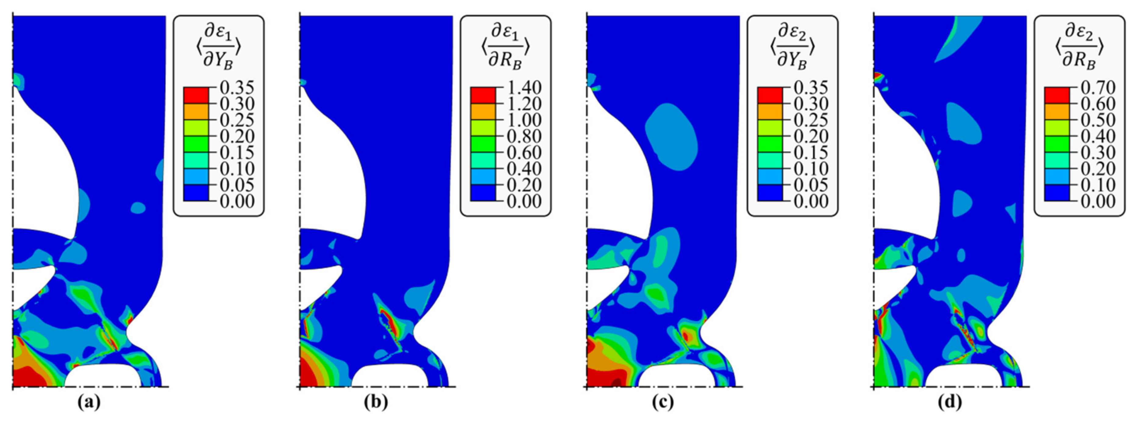
2.5. Sensitivity Analysis

The key feature of the sensitivity analysis is the specimen design. In the identification procedure, an issue might arise if the strain field is not sensitive to all sought parameters [38]. This means that some designs can result in lower accuracy of the identified parameters than others [34]. This issue has been addressed by Martins et al. [39] who studied the influence of different cruciform specimen geometries on the hardening and plastic anisotropy parameters. They found that VFM-based identification with specimen geometry proposed by Zhang et al. [40,41] yields a higher error on the shear parameter N in the Hill48 model in comparison to the other two proposed geometries and also with respect to other Hill’s parameters. A similar study was also conducted by Schmaltz and Willner [42], who tested even more sophisticated cruciform specimen designs. In their study, they show that FEMU-based identification fails at specimen tests that produce more features than the numerical material model can simulate. Moreover, to systematically tackle this issue, Souto et al. [43,44] proposed a quantitative indicator to distinguish, rate and rank different tests according to the strain state range, the deformation heterogeneity and the level of strain achieved.
In this study, a method used by Lecompte et al. [45,46] or Bertin et al. [47,48] is upgraded to evaluate how much the response of the heterogeneous strain specimen is sensitive to the sought parameters. In particular, the objective is to determine the sensitivity of principal strains ε 1 and ε 2 to variations in parameters Y B and R B . High sensitivity indicates that variation in a parameter results in a large variation in the strain field, whereas a small sensitivity suggests that variation in a parameter does not alter the simulated strain at all. Hence the parameter cannot be identified from the measured response. However, from the calculated sensitivity fields, it is also difficult to estimate which value is the bottom value if the sensitivities are not compared with some known value or being normalized. For these reasons, we calculated two types of sensitivities and normalized one with another.
Firstly, we calculated the sensitivity of heterogeneous specimen principal strain fields to parameter variations, i.e., ε 1 / Y B , ε 1 / R B , ε 2 / Y B and ε 2 / R B . Secondly, we analytically calculated the sensitivity of the standard uniaxial tensile test longitudinal strain ε 1 u n i to flow stress Y 0 variation and sensitivity of transversal strain ε 2 u n i to R 0 variation, i.e., ε 1 u n i / Y 0 , ε 2 u n i / R 0 . These two values will be used for normalization because it is well known that they are high in a uniaxial test. To derive the sensitivities ε 1 u n i / Y 0 , ε 2 u n i / R 0 , we assumed negligible elastic strains, plastic volume preservation, the proportionality of loading paths and that the uniaxial test is a force-driven process. Under these assumptions, a tensile force and R-value can be expressed as:
F 0 = Y 0 Y A 0 e ε 1 u n i ,         R 0 = ε 1 u n i ε 1 u n i + ε 2 u n i
where Y = Y ε e q p l presents reference flow stress, A 0 initial cross-section area and ε e q p l equivalent plastic strain. Furthermore, from the plastic work equivalence, i.e., Y ε e q p l = Y 0 Y ε 1 u n i , a relationship between ε 1 u n i and ε e q p l can be expressed as: ε e q p l = Y 0 ε 1 u n i . By taking a derivative of tensile force F 0 with respect to Y 0 , and setting it to zero, the sensitivity of the longitudinal strain ε 1 u n i to flow stress Y 0 variation ε 1 u n i / Y 0 can be expressed. Moreover, the sensitivity of transversal strain ε 2 u n i to R 0 variation can be derived from Equation (11), by expressing ε 2 u n i = R 0 ε 1 u n i 1 + R 0 1 and taking a derivative with respect to R 0 . Both results are given by the Equation (12).
ε 1 u n i Y 0 = Y + H ε e q p l Y H ,         ε 2 u n i R 0 = ε e q p l 1 + R 0 2 ,
where H presents hardening modulus and Y 0 is assumed to be one.
The sensitivities of the heterogeneous test, namely, ε 1 / Y B , ε 1 / R B , ε 2 / Y B and ε 2 / R B are evaluated numerically by using a forward difference scheme. With these values available, relative sensitivities can be expressed by:
ε i Y B = ε i / Y B ε 1 u n i / Y 0 = ε i Y B Y H Y + H ε e q p l ,       ε i R B = ε i / R B ε 2 u n i / R 0 = ε i R B 1 + R 0 2 ε e q p l ,     i 1 , 2 ,
where the values of Y ,   H and ε e q p l correspond to the current state of yielding. If no or only a small amount of equivalent plastic strain develops, the relative sensitivity is assumed to be zero.
The sensitivity fields are presented in Figure 3 and should be interpreted as information of ε 1 or ε 2 associated with parameters Y B or R B compared to the information from uniaxial test strains ε 1 or ε 2 associated with Y 0 or R 0 . From Figure 3a–d, it can be observed that maximum relative sensitivity is located mainly at the centre of the specimen and that the field is relatively uniformly distributed over the region. The localised peak values in Figure 3d originate as a numerical error when evaluating the relative sensitivities ε 1 / R B and ε 2 / R B at the points where material undergoes the elastic-plastic transition, after which the equivalent plastic strain is close to zero. No sensitivity is assumed at these locations because principal strains are also small.
However, Figure 3 indicates that all sensitivities of strain fields are accounted for strain acquisition points located at the centre of the specimen. In Figure 3a,c,d, it can be observed that sensitivities ε 1 / Y B , ε 2 / Y B and ε 2 / R B represent about 35% of sensitivities ε 1 / Y 0 or ε 2 / R 0 indicated by a standard uniaxial tensile test. Based on these values, it can be concluded that the parameters Y B and R B are well represented by the heterogeneous strain field test response at the centre of the specimen.
It is worth noting that the relative sensitivity of maximum principal strain ε 1 to variation in R B (Figure 3b) yields a value greater than one because variation in ε 1 in the biaxial state is larger than the variation in ε 2 in the uniaxial tensile test. It should also be noted that the maximum sensitivity in Figure 3c,d is located in the vicinity of the horizontal notch because the notch influences the principal stress direction, which means that ε 2 is pronounced.

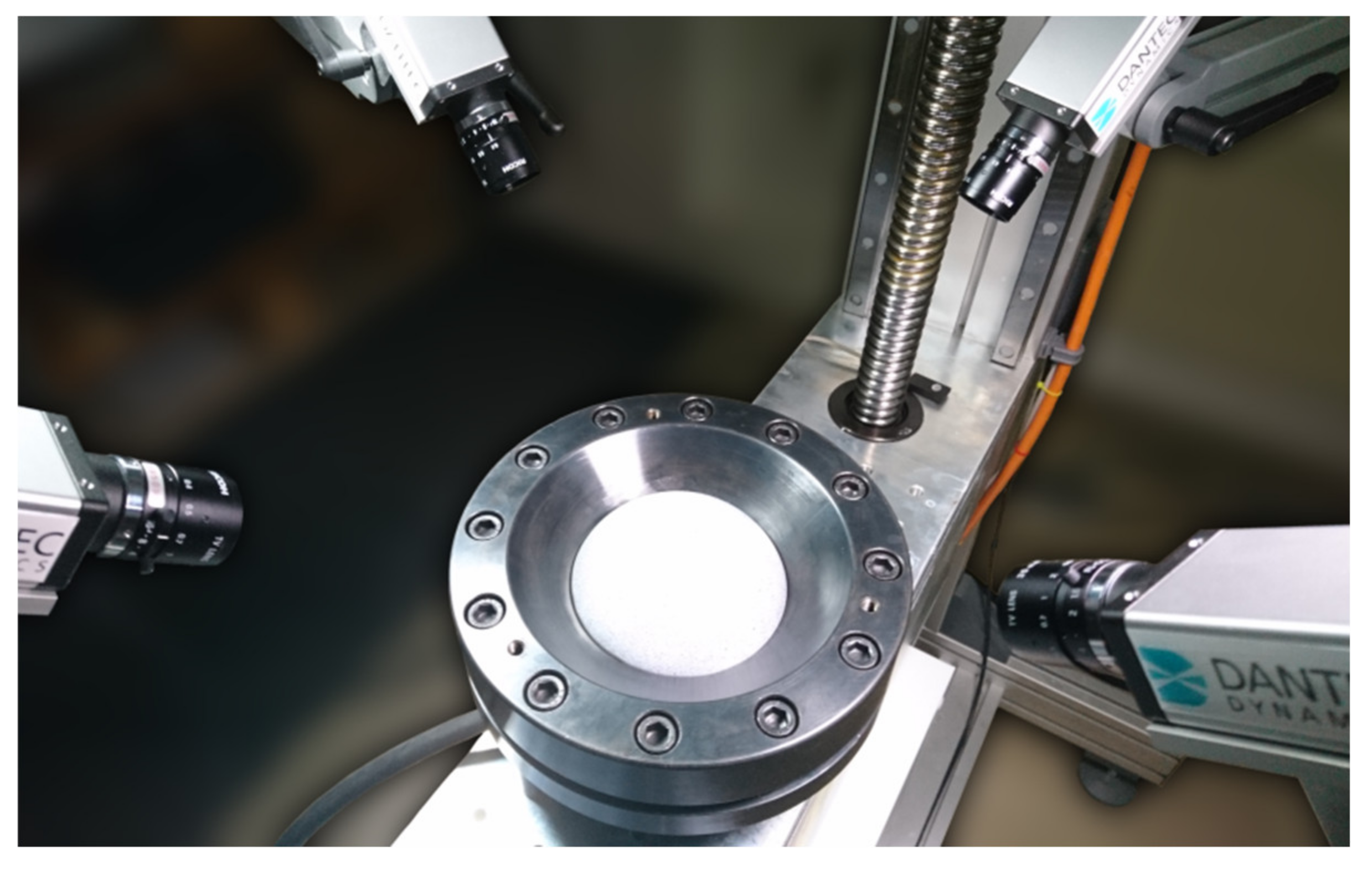
2.6. Experimental Procedure and Measurement of the Heterogeneous Test Response

The 304 austenitic stainless steel was chosen in this study, and its chemical composition was 0.07 C, 1.9 Mn, 19.2 Cr, 9.2 Ni, 0.04 P, 0.72 Si, 0.028 S, 0.09 N and balance Fe (wt. %). According to the proposed identification procedure, the standard uniaxial tensile tests [3] were carried out on 0.68 mm thick 304 stainless steel sheet metal in the parallel (0°), transverse (90°) and diagonal (45°) direction. Flow stress as a function of equivalent plastic strain and R-value in a selected direction were determined in accordance with the literature [49]. Flow curve in the rolling direction was set as a reference curve, meaning that the normalized flow stress Y 0 was set equal to unity. The normalized flow stresses in the other two directions, namely Y 90 and Y 45 , were determined by scaling the reference curve to the analysed curve and detailed information is available in Starman et al. [50]. The measured values are reported in the Results section.
The heterogeneous test specimens were cut using a wire electrical discharge machining process, where the specimens were cut in the rolling direction. To avoid excessive roughness and heat generation, which may influence the material properties, the cutting speed was 0.5 mm/h whereas the diameter of the cutting wire was 0.2 mm. The specimens are designed for use on a uniaxial tensile machine, therefore the geometry of the clamping part of the specimen is equal to the standard uniaxial tensile test. During the test, quasi-static loading conditions were imposed by tensile machine crosshead speed set equal to 0.01 mm/s and loading force measured with a 50 kN loading cell. The logarithmic surface strain field is measured at the centre of the specimen using a DIC optical system Q-400 Dantec Dynamics GmbH, (Ulm, Germany). The force measurement was synchronized with the acquisition of DIC images. The parameters of the optical measuring system are presented in Table 1.
Figure 4a presents the optical measurement system setup with multi-cam configuration, which is focused in the field of view 25 mm × 21 mm. In Figure 4b,c principal logarithmic strain fields ε 1 and ε 2 are presented, which are, for demonstration purposes only, measured over a larger field of view than finally selected (25 mm × 21 mm field of view). As shown, the fields are relatively homogeneous in the centre of the specimen, which means that the measurements are potentially less sensitive to strain location error. Based on this information, the principal strain fields ε 1 and ε 2 were measured in twelve acquisition points (cf. Figure 2c), which served in the inverse identification procedure. The measured force–strain responses are reported in the next section.

3. Results

In this section, the uniaxial test results and the heterogeneous specimen strain acquisition measurements are presented first. Based on these measurements, an inverse identification procedure is conducted, by comparison of measured and simulated strain field response. The results of the inverse identification are presented afterwards.

3.1. Standard Uniaxial Tensile Tests Results

Normalized flow stress values and width-to-thickness strain ratios measured from the standard uniaxial test were directly input into the conversion algorithm for YLD2000-2D model. The results are reported in Table 2. The left column presents normalized flow stresses and R-values, whereas the flow curve is given in the right column. The flow curve is calculated from the standard uniaxial test in the rolling direction as Y = F 0 / A , where A is the actual cross-section area. The equivalent plastic strain was calculated by ε e q p l = ε 1 u n i F 0 / E A , where the modulus of elasticity E was found to be 190 GPa.

3.2. Heterogeneous Strain Field Tensile Tests Results

The heterogeneous specimen logarithmic strain was measured at observation points presented in Figure 2c and plotted against tensile force. Due to the symmetric configuration of the acquisition points, the measurements were gathered in three characteristic points presented in Figure 5, which were processed for both principal surface strains.
Figure 5a corresponds to the middle, close-to-centre points (pt. 1, coloured red in Figure 2c), the centre column plot (Figure 5b) corresponds to the horizontal far-from-centre points (pt. 2, coloured green) and the right column plot (Figure 5c) corresponds to the vertical far-from-centre points (pt. 3, coloured blue in Figure 2c). Since three specimens were tested, this yielded twelve curves for each plot, and as seen from the figure, the discrepancy between the curves is within 5 × 10⁻⁴. This means that the repeatability of the measurements is high and that the specimens’ response is relatively symmetrical.

3.3. Identification Procedure Results

For the inverse identification process, finite element simulations of a heterogeneous specimen test were conducted in ABAQUS/Standard. A quarter model with 10,000 quadrilateral finite elements was used in the simulations. Logarithmic strain versus tensile force was monitored at the locations of characteristic points: pt. 1, pt. 2 and pt. 3. Furthermore, in the optimization procedure, the objective function was defined as a sum of the squared differences between the simulated and the measured data points of strain–force curves. The data of all six characteristic strain–force curves in the force range from 2.5 kN to 3.2 kN were included in the objective function definition. The gradient-based Levenberg-Marquardt optimization method was utilized to minimise the objective function, where the Jacobian matrix was calculated by the finite difference method. The identification procedure was started with initial values {1,1} for Y B and R B , and after three iterations, the minimum of the objective function was reached. The parameters are reported in Table 3. Moreover, because gradient methods are prone to reach local minima instead of a global one, the optimization process was repeated several times with different starting values. However, the same result Y B , R B = 0.94 , 1.03 was obtained each time in a few iterations.
By comparing the heterogeneous test responses in Figure 6, good agreement between simulated (solid line) and characteristic measured values (black dotted line) can be observed. The simulation results correspond to the identified parameters, given in Table 3. As shown, the simulation results fall within the standard deviation of the measurements.

3.4. Experimental Verification of Identified Anisotropy

The proposed methodology was verified by conducting a bulge test according to ISO 16808 [5], with which the identified values can be directly compared. The bulge tests (Figure 7) were performed using custom-built hydraulic testing equipment consisting of a chamfered die with a 160 mm opening and a circular steel base with a drawing bead to constrain sheet metal from moving towards the centre of the die. Before the pressurization, the die is tightened to the base plate with twelve bolts. During the pressure increase, the deformation of the bulge is monitored with a multi-cam DIC system which is synchronized with the pressure sensor. The multi-cam optical measuring setup is presented in Figure 7 and the settings were set to surpass the ISO 16808 optical system requirements. Three specimens were tested up to a pressure of 16 MPa at which no specimen rupture occurred. The strains were measured along with the sheet’s rolling and transverse-to-rolling direction.
The results are presented in Figure 8. Figure 8a presents the measured strains in the transverse direction ε T D plotted against the longitudinal strains ε R D . Linear regression is applied to the measured data points and the slope of the fit is defined as the value of R B e x p . The experimental value of this parameter was found to be 1.03, which is identical to the identified value in Table 3. Moreover, the hardening curve was calculated from the pressure and curvature measurement of the sheet, by following the procedure described in [51]. By using the bulge test, it was found that the yield curve is about 2 per cent lower than the reference curve obtained by the uniaxial test in the rolling direction. In other words, the conducted bulge test yields Y B e x p = 0.98 . By comparing this result with the value identified by the proposed procedure, it is found that there is approximately a 4% discrepancy between the measured and identified Y B value.

4. Discussion and Conclusions

This paper presents an alternative methodology for plastic anisotropy parameter calibration, which combines a heterogeneous strain field tensile test and a standard uniaxial tensile test, but avoids both special testing equipment for biaxial testing and a large number of identification parameters.
To avoid a large number of parameters in the identification procedure, the parameters of the employed model are first expressed as parameters with physical meaning using a conversion procedure. In this concept, the YLD2000-2d parameters α 1 ,   α 2 , , α 8 are first expressed with normalized flow stresses Y 0 ,     Y 90 ,   Y 45 ,   Y B and R-ratios, R 0 ,     R 90 ,   R 45 and R B . Moreover the flow stresses Y 0 e x p ,   Y 90 e x p ,   Y 45 e x p and width-to-thickness strain ratios   R 0 e x p ,     R 90 e x p ,   R 45 e x p , measured from the uniaxial tests, can be used directly as the model inputs. This way, the number of sought parameters can be reduced and the procedure substantially simplified.
For calibration, a heterogeneous strain field specimen for use on the standard tensile testing machine was designed. Although the specimen’s design is rather complicated, the geometry aims to induce pronounced biaxial state at the centre of the specimen, which is relatively uniformly distributed over the region. A disadvantage of the specimen is that it tends to buckle as the load increases. The strains in the specimen are relatively small, but this is a common issue of a majority of uniaxial heterogeneous field specimens because strain heterogeneity is usually achieved by the specimen’s shape heterogeneity. The latter induces stress concentrations at notches, which lead to premature necking of a specimen.
Although in our design the plastic strains are relatively small, this does not influence the identified R-value, because as demonstrated by the verification case, the biaxial R-value does not alter with the increased plastic strain substantially. On the other hand, a variation of R-values is usually common to uniaxial tensile tests. For example, as proposed by the standard procedure [4], the uniaxial R-values are measured in equivalent plastic strain range between 0.08 and 0.12 . If a heterogeneous testing procedure is aimed to identify these values and if the strains in a heterogeneous specimen are mainly small, unreliable results can be obtained.
Similar behaviour was anticipated also in the presented case, where the calculated strain field is influenced by the flow curve. In other words, it is known that flow stress can vary with increased plastic strain and better agreement between identified and measured normalized flow stress would be achieved with higher strains. The strains are relatively small, therefore we believe that this is the main reason for the discrepancy.
The employed sheet metal exhibits mild planar anisotropy, which results in biaxial R-value and normalized biaxial flow stress close to unity. Nevertheless, to verify the effectiveness, the optimization process was repeated several times with starting values changed up to 30%. The optimum was found in a few iterations. However, in the future, it would be valuable to validate the method with a sheet with stronger plastic anisotropy.
In the present work, eight material data are assumed to be available and the YLD2000-2d yield criterion is employed for anisotropy description. If the analysis is focused on materials having a strong planar anisotropy, more advanced yield criterion, e.g., YLD2004-18p [34,35] is suggested to be employed. Since with such a model more parameters have to be identified, additional uniaxial tests or upgraded heterogeneous strain field identification technique should be performed.

Author Contributions

Conceptualization, B.S. and A.M.; methodology, B.S.; software, A.M.; validation, A.M. and B.S.; formal analysis, B.S.; investigation, B.S. and A.M.; resources, M.H.; data curation, A.M. and M.H.; writing—original draft preparation, B.S. and A.M.; writing—review and editing, B.S., M.H. and N.M.; visualization, A.M.; supervision, N.M. and M.H.; project administration, N.M.; funding acquisition, M.H. All authors have read and agreed to the published version of the manuscript.

Funding

This research was funded by the Slovenian Research Agency, grant number P2-0263.

Acknowledgments

The authors acknowledge the financial support from the Slovenian Research Agency (research core funding No. P2-0263).

Conflicts of Interest

The authors declare no conflict of interest.

References

  1. Banabic, D. Sheet Metal Forming Processes: Constitutive Modelling and Numerical Simulation; Springer: Berlin/Heidelberg, Germany, 2010; ISBN 978-3-540-88112-4. [Google Scholar]
  2. Banabic, D.; Aretz, H.; Comsa, D.S.; Paraianu, L. An improved analytical description of orthotropy in metallic sheets. Int. J. Plast. 2005, 21, 493–512. [Google Scholar] [CrossRef]
  3. International Organization for Standardization. ISO 6892-1—Metallic Materials—Tensile Testing—Part 1: Method of Test at Room Temperature; International Organization for Standardization: Geneva, Switzerland, 2019. [Google Scholar]
  4. International Organization for Standardization. ISO 10113—Metallic Materials—Sheet and Strip—Determination of Plastic Strain Ratio; International Organization for Standardization: Geneva, Switzerland, 2006. [Google Scholar]
  5. International Organization for Standardization. ISO 16808—Determination of Biaxial Stress-Strain Curve by Means of Bulge Test with Optical Measuring System; International Organization for Standardization: Geneva, Switzerland, 2013. [Google Scholar]
  6. Barlat, F.; Brem, J.C.; Yoon, J.W.; Chung, K.; Dick, R.E.; Lege, D.J.; Pourboghrat, F.; Choi, S.-H.; Chu, E. Plane stress yield function for aluminum alloy sheets—Part 1: Theory. Int. J. Plast. 2003, 19, 1297–1319. [Google Scholar] [CrossRef]
  7. Merklein, M.; Kuppert, A. A method for the layer compression test considering the anisotropic material behavior. Int. J. Mater. Form. 2009, 2, 483. [Google Scholar] [CrossRef]
  8. International Organization for Standardization. ISO 16842—Metallic Materials—Sheet and Strip—Biaxial Tensile Testing Method Using a Cruciform Test Piece; International Organization for Standardization: Geneva, Switzerland, 2014. [Google Scholar]
  9. Kuwabara, T. Advances in experiments on metal sheets and tubes in support of constitutive modeling and forming simulations. Int. J. Plast. 2007, 23, 385–419. [Google Scholar] [CrossRef]
  10. Merklein, M.; Biasutti, M. Development of a biaxial tensile machine for characterization of sheet metals. J. Mater. Process. Technol. 2013, 213, 939–946. [Google Scholar] [CrossRef]
  11. Fu, J.; Barlat, F.; Kim, J.-H. Parameter identification of the homogeneous anisotropic hardening model using the virtual fields method. Int. J. Mater. Form. 2016, 9, 691–696. [Google Scholar] [CrossRef]
  12. Pottier, T.; Vacher, P.; Toussaint, F.; Louche, H.; Coudert, T. Out-of-plane Testing Procedure for Inverse Identification Purpose: Application in Sheet Metal Plasticity. Exp. Mech. 2012, 52, 951–963. [Google Scholar] [CrossRef]
  13. Mathieu, F.; Leclerc, H.; Hild, F.; Roux, S. Estimation of Elastoplastic Parameters via Weighted FEMU and Integrated-DIC. Exp. Mech. 2015, 55, 105–119. [Google Scholar] [CrossRef]
  14. Kajberg, J.; Lindkvist, G. Characterisation of materials subjected to large strains by inverse modelling based on in-plane displacement fields. Int. J. Solids Struct. 2004, 41, 3439–3459. [Google Scholar] [CrossRef]
  15. Latourte, F.; Chrysochoos, A.; Pagano, S.; Wattrisse, B. Elastoplastic Behavior Identification for Heterogeneous Loadings and Materials. Exp. Mech. 2008, 48, 435–449. [Google Scholar] [CrossRef]
  16. Grédiac, M.; Pierron, F. Applying the Virtual Fields Method to the identification of elasto-plastic constitutive parameters. Int. J. Plast. 2006, 22, 602–627. [Google Scholar] [CrossRef]
  17. Pierron, F.; Avril, S.; Tran, V.T. Extension of the virtual fields method to elasto-plastic material identification with cyclic loads and kinematic hardening. Int. J. Solids Struct. 2010, 47, 2993–3010. [Google Scholar] [CrossRef] [Green Version]
  18. Claire, D.; Hild, F.; Roux, S. A finite element formulation to identify damage fields: The equilibrium gap method. Int. J. Numer. Methods Eng. 2004, 61, 189–208. [Google Scholar] [CrossRef] [Green Version]
  19. Rossi, M.; Broggiato, G.B.; Papalini, S. Application of digital image correlation to the study of planar anisotropy of sheet metals at large strains. Meccanica 2008, 43, 185–199. [Google Scholar] [CrossRef]
  20. Rossi, M.; Lattanzi, A.; Barlat, F. A general linear method to evaluate the hardening behaviour of metals at large strain with full-field measurements. Strain 2018, 54, e12265. [Google Scholar] [CrossRef]
  21. Avril, S.; Bonnet, M.; Bretelle, A.S.; Grediac, M.; Hild, F.; Ienny, P.; Latourte, F.; Lemosse, D.; Pagano, S.; Pagnacco, E.; et al. Overview of identification methods of mechanical parameters based on full-field measurements. Exp. Mech. 2008. to appear. [Google Scholar] [CrossRef] [Green Version]
  22. Meuwissen, M.H.H.; Oomens, C.W.J.; Baaijens, F.P.T.; Petterson, R.; Janssen, J.D. Determination of the elasto-plastic properties of aluminium using a mixed numerical–experimental method. J. Mater. Process. Technol. 1998, 75, 204–211. [Google Scholar] [CrossRef]
  23. Haddadi, H.; Belhabib, S. Improving the characterization of a hardening law using digital image correlation over an enhanced heterogeneous tensile test. Int. J. Mech. Sci. 2012, 62, 47–56. [Google Scholar] [CrossRef]
  24. Robert, L.; Velay, V.; Decultot, N.; Ramde, S. Identification of hardening parameters using finite element models and full-field measurements: Some case studies. J. Strain Anal. Eng. Des. 2012, 47, 3–17. [Google Scholar] [CrossRef]
  25. Güner, A.; Soyarslan, C.; Brosius, A.; Tekkaya, A.E. Characterization of anisotropy of sheet metals employing inhomogeneous strain fields for Yld2000-2D yield function. Int. J. Solids Struct. 2012, 49, 3517–3527. [Google Scholar] [CrossRef] [Green Version]
  26. Kim, J.-H.; Barlat, F.; Pierron, F.; Lee, M.-G. Determination of Anisotropic Plastic Constitutive Parameters Using the Virtual Fields Method. Exp. Mech. 2014, 54, 1189–1204. [Google Scholar] [CrossRef]
  27. Kowalewski, Ł.; Gajewski, M. Assessment of Optimization Methods Used to Determine Plasticity Parameters Based on DIC and back Calculation Methods. Exp. Tech. 2019, 43, 385–396. [Google Scholar] [CrossRef] [Green Version]
  28. Cooreman, S.; Lecompte, D.; Sol, H.; Vantomme, J.; Debruyne, D. Identification of Mechanical Material Behavior Through Inverse Modeling and DIC. Exp. Mech. 2008, 48, 421–433. [Google Scholar] [CrossRef]
  29. Denys, K.; Coppieters, S.; Seefeldt, M.; Debruyne, D. Multi-DIC setup for the identification of a 3D anisotropic yield surface of thick high strength steel using a double perforated specimen. Mech. Mater. 2016, 100, 96–108. [Google Scholar] [CrossRef]
  30. Martins, J.M.P.; Andrade-Campos, A.; Thuillier, S. Comparison of inverse identification strategies for constitutive mechanical models using full-field measurements. Int. J. Mech. Sci. 2018, 145, 330–345. [Google Scholar] [CrossRef]
  31. Rossi, M.; Pierron, F. Identification of plastic constitutive parameters at large deformations from three dimensional displacement fields. Comput. Mech. 2012, 49, 53–71. [Google Scholar] [CrossRef] [Green Version]
  32. Rossi, M.; Pierron, F.; Štamborská, M. Application of the virtual fields method to large strain anisotropic plasticity. Int. J. Solids Struct. 2016, 97–98, 322–335. [Google Scholar] [CrossRef]
  33. Lattanzi, A.; Barlat, F.; Pierron, F.; Marek, A.; Rossi, M. Inverse identification strategies for the characterization of transformation-based anisotropic plasticity models with the non-linear VFM. Int. J. Mech. Sci. 2020, 105422. [Google Scholar] [CrossRef]
  34. Barlat, F.; Yoon, J.W.; Cazacu, O. On linear transformations of stress tensors for the description of plastic anisotropy. Int. J. Plast. 2007, 23, 876–896. [Google Scholar] [CrossRef]
  35. Barlat, F.; Aretz, H.; Yoon, J.W.; Karabin, M.E.; Brem, J.C.; Dick, R.E. Linear transformation-based anisotropic yield functions. Int. J. Plast. 2005, 21, 1009–1039. [Google Scholar] [CrossRef]
  36. Marek, A.; Davis, F.M.; Rossi, M.; Pierron, F. Extension of the sensitivity-based virtual fields to large deformation anisotropic plasticity. Int. J. Mater. Form. 2019, 12, 457–476. [Google Scholar] [CrossRef] [Green Version]
  37. Marek, A.; Davis, F.M.; Pierron, F. Sensitivity-based virtual fields for the non-linear virtual fields method. Comput. Mech. 2017, 60, 409–431. [Google Scholar] [CrossRef] [PubMed] [Green Version]
  38. Badaloni, M.; Rossi, M.; Chiappini, G.; Lava, P.; Debruyne, D. Impact of Experimental Uncertainties on the Identification of Mechanical Material Properties using DIC. Exp. Mech. 2015, 55, 1411–1426. [Google Scholar] [CrossRef]
  39. Martins, J.M.P.; Andrade-Campos, A.; Thuillier, S. Calibration of anisotropic plasticity models using a biaxial test and the virtual fields method. Int. J. Solids Struct. 2019, 172–173, 21–37. [Google Scholar] [CrossRef]
  40. Zhang, S.; Leotoing, L.; Guines, D.; Thuillier, S.; Zang, S. Calibration of anisotropic yield criterion with conventional tests or biaxial test. Int. J. Mech. Sci. 2014, 85, 142–151. [Google Scholar] [CrossRef] [Green Version]
  41. Zhang, S.Y.; Leotoing, L.; Guines, D.; Thuillier, S. Identification of Anisotropic Yield Criterion Parameters from a Single Biaxial Tensile Test. Key Eng. Mater. 2014, 611–612, 1710–1717. [Google Scholar] [CrossRef] [Green Version]
  42. Schmaltz, S.; Willner, K. Comparison of Different Biaxial Tests for the Inverse Identification of Sheet Steel Material Parameters. Strain 2014, 50, 389–403. [Google Scholar] [CrossRef]
  43. Souto, N.; Thuillier, S.; Andrade-Campos, A. Design of an indicator to characterize and classify mechanical tests for sheet metals. Int. J. Mech. Sci. 2015, 101–102, 252–271. [Google Scholar] [CrossRef]
  44. Souto, N.; Andrade-Campos, A.; Thuillier, S. A numerical methodology to design heterogeneous mechanical tests. Int. J. Mech. Sci. 2016, 107, 264–276. [Google Scholar] [CrossRef]
  45. Lecompte, D.; Cooreman, S.; Coppieters, S.; Vantomme, J.; Sol, H.; Debruyne, D. Parameter identification for anisotropic plasticity model using digital image correlation. Eur. J. Comput. Mech. 2009, 18, 393–418. [Google Scholar]
  46. Lecompte, D.; Smits, A.; Sol, H.; Vantomme, J.; Van Hemelrijck, D. Mixed numerical–experimental technique for orthotropic parameter identification using biaxial tensile tests on cruciform specimens. Int. J. Solids Struct. 2007, 44, 1643–1656. [Google Scholar] [CrossRef] [Green Version]
  47. Bertin, M.; Hild, F.; Roux, S. On the identifiability of Hill-1948 plasticity model with a single biaxial test on very thin sheet. Strain 2017, 53, e12233. [Google Scholar] [CrossRef] [Green Version]
  48. Bertin, M.; Hild, F.; Roux, S. On the identifiability of the Hill-1948 model with one uniaxial tensile test. Comptes Rendus Mécanique 2017, 345, 363–369. [Google Scholar] [CrossRef]
  49. Davis, J.R. Tensile Testing, 2nd ed.; ASM International: Materials Park, OH, USA, 2004; ISBN 978-1-61503-095-8. [Google Scholar]
  50. Starman, B.; Vrh, M.; Koc, P.; Halilovič, M. Shear test-based identification of hardening behaviour of stainless steel sheet after onset of necking. J. Mater. Process. Technol. 2019, 270, 335–344. [Google Scholar] [CrossRef]
  51. Suttner, S.; Merklein, M. Experimental and numerical investigation of a strain rate controlled hydraulic bulge test of sheet metal. J. Mater. Process. Technol. 2016, 235, 121–133. [Google Scholar] [CrossRef]
Figure 1. Proposed calibration procedure using standard uniaxial tensile tests and purposely developed heterogeneous test: (a) required experimental tests, (b) conversion of parameters Y 0 ,     Y 90 ,   Y 45 ,   R 0 ,   R 90 , R 45 ,   Y B ,   R B to YLD2000-2d parameters α 1 ,   α 2 , , α 8 , (c) numerical simulation of heterogeneous test response, (d) calculated and (e) measured heterogeneous test responses are compared in (f) the inverse identification procedure.
Metals 10 00542 g001
Figure 2. The geometry of the purposely developed heterogeneous test for use on a standard uniaxial testing machine: (a) shape with overall dimensions, (b) detailed section, (c) location of twelve strain acquisition points at the centre of the specimen.
Metals 10 00542 g002
Figure 3. Heterogeneous test relative sensitivity fields: (a) relative sensitivity of max. principal strain ε 1 to a change of Y B , (b) relative sensitivity of max. principal strain ε 1 to a change of R B , (c) relative sensitivity of min. principal strain ε 2 to a change of Y B , (d) relative sensitivity of min. principal strain ε 2 to a change of R B .
Metals 10 00542 g003
Figure 4. Heterogeneous specimen strain field measurement: (a) optical measurement system with a multi-cam configuration, (b) measured maximum principal logarithmic surface strain field contours ε 1 (c) measured minimum principal logarithmic surface strain field contours ε 2 .
Metals 10 00542 g004
Figure 5. Characteristic measurements of heterogeneous specimen response: (a) max./min. strain–force response at the close-to-centre points (pt. 1), (b) max./min. strain–force response at the horizontal far-from-centre points (pt. 2), (c) max./min. strain–force response at the vertical far-from-centre points (pt. 3). Blue and red insets in the figure represent the central region in Figure 4b,c, whereas the acquisition points are coloured red, green and blue. Short cyan lines represent the direction of a principal strain.
Metals 10 00542 g005
Figure 6. Comparison of simulated and measured responses of the heterogeneous specimen test: (a) max./min. strain–force response at the close-to-centre points (pt. 1), (b) max./min. strain–force response at the horizontal far-from-centre points (pt. 2), (c) max./min. strain–force response at the vertical far-from-centre points (pt. 3).
Metals 10 00542 g006
Figure 7. Bulge test setup with optical measurement equipment in the multi-cam configuration.
Metals 10 00542 g007
Figure 8. Bulge test results: (a) transverse direction strain ε T D as a function of rolling direction strain ε R D , (b) yield curve as a function of equivalent plastic strain calculated from the bulge test.
Metals 10 00542 g008
Table 1. Adopted Digital Image Correlation (DIC) settings for the heterogeneous test.
camerasManta G-507, Allied Vision, (Exton, PA, USA) (3 pieces)
image resolution2464 pixel × 2056 pixel
objective focal distance35 mm
field of view25 mm × 21 mm
stereo angle80° (between outermost cameras)
patterning techniquematt white spray paint base coat with black speckles
pattern feature size (approx.)3 pixel
DIC techniquemulti-cam
DIC softwareIstra 4D (ver. 4.4.6), Dantec Dynamics GmbH, (Ulm, Germany)
facet size19 pixel
grid spacing12 pixel
spatial smoothinglocal regression (5 × 5 window)
temporal smoothingnone
logarithmic strain noise-floor5 × 10−4
number of acquired data points16,000
acquisition frequency2 Hz
Table 2. Normalized flow stresses, R-values and plastic flow curve calculated from the uniaxial tensile test data. Nine specimens were tested for each cutting direction.
Normalized Flow Stress and R-ValueIsotropic Hardening
Y ε e q p l    MPa Y ε e q p l    MPa
Y 0 1.00 Y 0 213 Y (2.0e-2)368
Y 90 1.03 Y (3.0e-4)255 Y (5.0e-2)446
Y 45 0.98 Y (9.0e-4)284 Y (1.0e-1)564
R 0 0.92 Y (3.0e-3)300 Y (1.5e-1)665
R 90 0.81 Y (6.0e-3)317 Y (2.0e-1)760
R 45 1.21 Y (1.0e-2)333 Y (3.0e-1)940
Table 3. The values of identified parameters using a heterogeneous test response.
Identified Parameters
Y B 0.94
R B 1.03

