Article

Multi-Criteria Selection of the Optimal Parameters for High-Speed Machining of Aluminum Alloy Al7075 Thin-Walled Parts

1
Department of Production Engineering, Faculty of Technical Sciences, University of Novi Sad, 21000 Novi Sad, Serbia
2
Department of Machining, Assembly and Engineering Metrology, Faculty of Mechanical Engineering, Technical University of Ostrava, 70800 Ostrava, Czech Republic
3
Department of Mechanical Engineering, Technical Faculty “Mihajlo Pupin”, University of Novi Sad, 23000 Zrenjanin, Serbia
*
Author to whom correspondence should be addressed.
Metals 2020, 10(12), 1570; https://doi.org/10.3390/met10121570
Submission received: 19 October 2020 / Revised: 18 November 2020 / Accepted: 22 November 2020 / Published: 24 November 2020
(This article belongs to the Special Issue Heat Treatment and Mechanical Properties of Metals and Alloys)

Abstract

:
Thin-walled parts made of aluminum alloy are mostly used as structural elements in the aerospace, automobile, and military industries due to good homogeneity, corrosion resistance, and the excellent ratio between mechanical properties and mass. Manufacturing of these parts is mainly performed by removing a large volume of material, so it is necessary to choose quality machining parameters that will achieve high productivity and satisfactory quality and accuracy of machining. Using the Taguchi methodology, an experimental plan is created and realized. Based on its results and comparative analysis of multi-criteria decision making (MCDM) methods, optimal levels of machining parameters in high-speed milling of thin-walled parts made of aluminum alloy Al7075 are selected. The varying input parameters are wall thickness, cutting parameters, and tool path strategies. The output parameters are productivity, surface quality, dimensional accuracy, the accuracy of forms and surface position, representing the optimization criteria. Selection of the optimal machining parameter levels and their ranking is realized using 14 MCDM methods. Afterward, the obtained results are compared using correlation analysis. At the output, integrative decisions were made on selecting the optimal level and rank of alternative levels of machining parameters.

1. Introduction

The modern market of specialized products requires materials with high mechanical properties, small mass, relatively low price, and good machinability, which is all contained in aluminum alloys [1]. Thin-walled parts of aluminum alloys are very important structural components in the aerospace, automobile, and military industries, but they are often used in toolmaking and other electromechanical industry branches [2,3].
In parallel with the increase in market requirements for thin-walled components of aluminum alloys, numerous studies are being realized which are oriented towards:
  • Design optimization to reduce mass, deformations and vibrations, increase load capacity, and strength
  • Optimization of manufacturing process planning to increase productivity, cost-effectiveness, the dimensional accuracy, accuracy of forms and surface position, machining quality, etc., which is the main research subject in this paper.
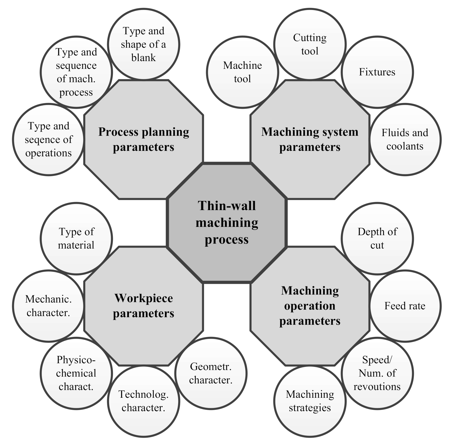
Thin-walled parts of Al alloys can be obtained by casting, injection molding, material removal technologies, etc. Manufacturing of these parts is most often realized by milling, during which a large volume of material is removed, which can amount up to 95% of the initial mass of raw material [4,5]. Therefore, using appropriate high-speed machining parameters, it is necessary to achieve high productivity while also maintaining the required machining accuracy and quality. On the other hand, due to the low stiffness of thin-walls, it is also recommended to avoid the appearance of vibrations and deformations, which can cause machining errors, low quality, and the appearance of scrap [6,7,8,9]. The main causes for the appearance of these errors in the literature are the type of material, elements of machining system (machine, tool, fixtures), cutting parameters, machining strategies, metalworking fluids and coolants, wall thickness, and others [2,5,10,11,12,13,14,15]. By analyzing numerous research studies, influential machining parameters for thin-walled structures are systematized and represented in Figure 1.
The main groups of machining parameters for thin-walled parts are the following:
  • Process planning parameters: Type and shape of a blank (casting, bar, sheet metal, etc.), Type and sequence of process operations (casting, cutting, heat treatment, etc.), Type and sequence of machining operations (face and plane milling, rough and soft milling, etc.)
  • Machining system parameters: Machine tool (stiffness, accuracy, available cutting parameters, etc.), Cutting tool (type, material, geometry, number of cutting edges, specific cutting edge angles, etc.), Fixtures (type, method, and place of positioning, clamping force, etc.), Metalworking fluids and coolants (type, concentration, purity, supply method, pressure)
  • Workpiece parameters: Type of material, Mechanical characteristics (hardness, strength, elasticity, toughness, etc.), Physicochemical characteristics (structure, chemical composition, density, thermal characteristics, corrosion resistance, etc.), Technological characteristics (machinability parameters), Geometric characteristics (shape: linear, triangular, rectangular, hexagonal and complex; wall-thickness to the wall-height ratio: small height-to-thickness ratio <15:1, moderate height-to-thickness ratio <30:1, very large height-to-thickness ratio ≥30:1; the accuracy of measures, the accuracy of forms and surface position; surface quality, etc.) and
  • Machining operation parameters: depth of cut, feed, cutting speed/number of revolutions, tool path strategies.
Authors in [16,17] investigated the influence of wall thickness, milling forces, and cutting tool position on the deformations of thin-walls and the appearance of geometric errors. The results from [16] show that the machining parameters can be selected for each pass to achieve milling efficiency and accuracy, while the results from [17] predict the definition of remnant material in order to reduce deformations and achieve high machining quality. Yan et al. [18] proposed the machining strategy with maximal depth of cut from the considered range and with the respect to the threshold of the cutting force. Efficiency of the proposed methodology was tested on the basis of simulation and experiments and the obtained results showed the reduction in machining time and surface error.
The study in [19] considers the influence of clamping fixtures, operation sequence, selected tool path strategy, and cutting parameters on plastic/elastic deformations during the machining process using FEM analysis and CAM software. The proposed model performs a computationally efficient transient thermo-mechanical coupled field milling simulation, predicts the workpiece non-linear behavior during machining due to its changing geometry, allows the modelling of the effects of initial residual stresses on part deformations and integrated analytical machining load - cutting force and shear plane temperature. A model of deformations of thin-walled structures in the milling process and prediction of machining errors are investigated in [20,21]. In [20], a new model is proposed to predict surface form errors caused by milling force during the five-axis flank milling process. The results showed that the surface deformation error of thin-walled structures is affected together by the instantaneous milling force and the local stiffness of the workpiece. On the other hand, in the paper [21] a three-dimensional finite element model was established for the milling of thin-walled parts, that predicts the elastic deformation law of the thin-walled blade.
Sapthagiri and Rao [22] used the Taguchi method to experimentally examine the significance of machining parameters (cutting speed, feed, depth of cut, a width of cut, tool path layout) and the influence of coolants on the reduction in tool temperature, as influential parameters on the deformation during machining. The optimum parameters which influence distortion were identified. By checking the samples machining with different tools and different speeds the warpage of the components are very less. Authors in [23] emphasized the influence of cutting parameters on the cutting forces and the surface roughness during face milling of aluminum alloy 7075 obtained by the new semi-solid metal casting process. Results show that the optimal combination for the cutting force is the choice of a minimum level for all tested parameters, while for the surface roughness the cutting depth at the median level is the most preferable for the observed range.
Sridhar and Babu [24] investigated the influence of the material removal rate on the distortion of thin-walled parts of aluminum alloy by combining the following machining parameters: feed, cutting speed, depth of cut, and width of cut. They concluded that the increase of feed, depth of cut and width of cut lead to the increase of distortion of thin-walled structures. Also, the increase of material removal rate by increasing feed and speed instead of depth of cut and width of cut represents better solution for minimizing wall distortion. Qu et al. [25] optimized the milling parameters for thin-walled parts from the point of view of cutting forces, surface roughness, and material removal rate. The results showed that the cutting force and surface roughness increased with increasing feed per tooth and milling depth. On the other hand, the increase of spindle speed affected the increase of cutting force as well as the decrease of surface roughness.
Bolar et al. [26] researched the influence of feed rate, the number of flutes and machining strategies on surface finish, and deflection errors during machining of ultra-thin C shaped walls made of aluminum alloy. The authors concluded that a combined approach i.e., concave and convex machining with four fluted carbide end mill produced superior quality and precise thin-wall components. Shamsuddin et al. [27] compared milling cutting path strategies on surface finish, thickness accuracy, and machining time for thin-walled aluminum alloys. MasterCam X MR2 software was used to obtain the best tool path strategy. Experimental results showed that true spiral is the best machining strategy in terms of thickness accuracy but lack of surface roughness when compared to other machining strategies. However, concerning surface roughness and machining time, the parallel spiral strategy was more promising when compared to other strategies. Popma [28] developed a system for automated generative computer-aided process planning (CAPP) for thin-walled parts machined on high-speed CNC machines with a special emphasis on machining sequence and strategies for thin-walled parts while achieving accuracy and quality of machining.
Due to the low rigidity of the thin-walled structures, vibrations often occur during machining, which is divided into self-induced and forced vibrations [5]. Self-induced vibrations or chatter occur when the frequency response is induced by the machining process, i.e., due to friction in the tool-workpiece system, thermo-mechanical processes, or as a consequence of a regenerative effect. Forced vibrations or amplification occur when the stiffness of the part is not sufficient to maintain a constant chip thickness. The cutting tool bounces off the workpiece, producing vibrations at the same frequency as the main spindle and its components.
Machining parameters significantly affect the efficiency of the machining process but also its stability. In order to provide these criteria stability lobes diagrams (SLD) are used. Stability lobes diagrams represent areas of stability, i.e., areas of machining parameters where vibrations will not occur [29]. Authors in [30] studied the effect of VSR (Vibratory Stress Relief) on the deformations and residual stresses of Al 7075 thin-walled parts. They concluded that VSR improved the shape and size of material stability to a significant level by relieving induced residual stresses in thin-walled parts. In addition to static and dynamic models, there are also analytical models related to the development of new methods for predicting the behavior of systems based on frequency response and deformations resulting from cutting forces [31].
By analyzing the literature sources, it can be concluded that the field of machining of thin-walled parts has been the research subject of many researchers around the world for many years. Due to the specificity of the thin-walled part design, the machining parameters’ influence is much more pronounced compared to the “normal” thick-walled parts. Optimization theory as a scientific discipline has a huge application in solving various engineering problems, where the application of appropriate methods finds the best solution for the selected optimization object for certain conditions based on one or more optimization criteria. Machining parameters are most often input variables that are optimized within the machining processes. For optimal parameters, those values are taken that give the best solution of the objective function. The selection and optimization of machining parameters are mostly realized using experimental research with the application of appropriate single and multi-criteria optimization methods, simulation techniques, and their combination.
This paper’s main research subject is to determine the quality machining parameters in high-speed milling of linear thin-walled components made of aluminum alloy Al7075. To that end, using the standard Taguchi orthogonal sequence L27, the experimental plan is created and realized. Based on its results and by applying MCDM methods, selecting the optimum machining parameter levels is achieved. At the input of the experimental design, the following parameters are varied: wall thickness (a), number of revolutions (n), feed rate (f), depth of cut (δ), and tool path strategies (TPS), while the output parameters are the following ones: machining time (T)/material removal rate (MRR), wall thickness deviation (Δa), flatness deviation (Δb), parallelism deviation (Δc), perpendicularity deviation (Δd) and surface roughness (Ra). These output parameters represent the optimization criteria, which are assigned weight coefficients based on the design and technological requirements of thin-walled parts. The selection of the optimum machining parameter levels and their ranking is realized using 14 chosen MCDM methods: GRA (Grey Relational Analysis), AHP (Analytic Hierarchy Process), MOORA (Multi-Objective Optimization Method by Ratio Analysis), TOPSIS (Technique for Order Performance by Similarity to Ideal Solution), ROV (Range Of Value), COPRAS (COmplex PRoportional Assessment of alternatives), ARAS (Additive Ratio ASsessment), WASPAS (Weighted Aggregates Sum Product ASsessment), VIKOR (VIsekriterijumska optimizacija i KOmpromisno Resenje - in Serbian), OCRA (Operational Competitiveness Rating Analysis), EDAS (Evaluation based on Distance from Average Solution), MABAC (Multi-Attributive Border Approximation area Comparison), SAW (Simple Additive Weighting) and SPW (Simple Product Weighting). The obtained results are compared and methods that satisfy the pre-determined constraints of correlation coefficients are adopted using correlation analysis. Based on these results, the integrative and final solution of the optimal machining parameter levels is defined, and alternative solutions are ranked.

2. MCDM Problem and the Model of the Integrative Multi-Criteria Ranking of Alternatives

2.1. MCDM Problem

Designers often encounter the need to select the optimal solution concerning products, processes, resources, etc. [32,33]. In such situations, in addition to a large number of alternatives, a large number of criteria appear, which together make the problem of selection more complex. The appearance of several alternatives and criteria, some of which need to be maximized and some minimized, means that decisions should be made in conflicting conditions and that multi-criteria decision-making techniques should be applied to solve these complex tasks. These methods are based on scientific principles that efficiently determine the optimal solution [34,35].
Since the proposed decision-making problem refers to the limited number of known alternatives, the application of multiple-attribute decision making (MADM) is assumed. Numerous researchers and scientists have developed many MCDM methods, from intuitive to sophisticated analytical methods. These methods can be used to identify a single most suitable alternative, rank alternatives, select a limited number of alternatives, or simply to distinguish acceptable from unacceptable alternatives [32,34].
There are similarities and differences when dividing the decision-making process into phases, but they can generally be divided into the following ones:
  • Identifying and formulating a decision-making problem—an objective function;
  • Forming a decision-making model—determining a set of alternatives and criteria and collecting appropriate data;
  • Applying an MCDM method—determining weight coefficients, evaluating alternatives for selected criteria and evaluating alternatives;
  • Selecting the most acceptable alternative and/or ranking alternatives;
  • Correlation analysis and integrative selection of the most acceptable alternative and/or ranking of alternatives (in case of using several MCDM methods to solve the same problem);
  • Analyzing the obtained results.
MCDM is a scientific field that is growing rapidly and intensively, as evidenced by the numerous methods that have been developed so far and are still being developed [32,34,36,37,38,39,40,41,42]. In this paper, the following MCDM methods introduced by the following researchers are applied: GRA [43], AHP [44], MOORA [45], TOPSIS [46], ROV [47], COPRAS [48], ARAS [49], WASPAS [50], VIKOR [51], OCRA [52], EDAS [53,54], MABAC [55], SAW [56] and SPW [34]. The main characteristics of these methods are to be transparent and simple, provide a complete ranking of alternatives, ensure the use of minimum and maximum criteria, enable the use of quantitative and qualitative data, not to require expert knowledge in mathematics, and not to use specialized software [32,34,38].
In most papers, one or a few MCDM methods are used to select the optimal variant of products, processes, resources, materials, etc. When a large number of these methods are applied, it is necessary to compare them and make a final integrative decision about the selection of the optimal solution [34,57,58,59].

2.2. Model of the Integrative Multi-Criteria Ranking of Alternatives

By applying several different MCDM methods to the same problem, even the same decision-maker can obtain different results of alternative rankings which leads to the problem of conflicting decision results. To be able to statistically analyze these conflicts and select methods whose results will be the basis for deciding and selecting the optimal alternative and their rank, it is necessary to consider as many different methods as possible that would form a sufficient sample [34,57,58,59].
To reduce the risk of making wrong decisions, a large number of different MCDM methods are applied in this paper. Through an iterative procedure, it is necessary to choose at least two methods that will form the basis for integrative decision making on selecting the optimal alternative and rank of alternatives. In the proposed case, these methods are chosen using the following methodology which is realized through several iterations based on the appropriate parameters of correlation with the limit values.

2.2.1. First Iteration

In the first iteration, the ranks of all applied MCDM methods are compared, and the values of Spearman’s rank correlation coefficients (Ri), the total Kendall’s rank correlation coefficient (W) as well as the average Spearman rank correlation coefficient (R) of all MCDM methods are determined, as well as standard deviations for all levels (σi), i.e., values of maximum and average standard deviation (σmax and σav). These coefficients are compared with the limit-acceptable values, and if they are all within the allowed limits, no further iterations will be performed. On the other hand, the final solution—the ranks of alternative levels of a process plan’s parameters can be formulated.

Spearman’s Rank Correlation Coefficient (Ri)

Spearman’s rank correlation coefficient (Ri) makes it possible to quantify the degree of correlation between any two sets of rank alternatives obtained by applying different MCDM methods and is calculated according to the Equation (1). Spearman’s rank correlation coefficients (Ri) should be in the range between 0.9 ≤ Ri ≤ 1 [60].
R i = 1 6 i = 1 N d i 2 N N 2 1
where:
  • N—sample size (number of alternatives to be ranked);
  • Xi and Yi—the calculation values of output coefficients for any two MCDM methods;
  • xi and yi—the ranks of alternatives in the model obtained based on Xi and Yi values;
  • di = (xi − yi)—the difference between ranks of alternatives of two MCDM methods.

Kendall’s Rank Correlation Coefficient

Kendall’s rank correlation coefficient is used to determine the degree of correlation of the ranks of all alternatives when three or more MCDM methods are used for decision making, which corresponds to the case investigated in this paper. Kendall’s rank correlation coefficient (W) is calculated using the Equation (2). Kendall’s rank correlation coefficient should be in the range between 0.9 ≤ W ≤ 1 [61]:
W = 12 · i = 1 k T j 2 k 2 · m m 2 1 3 m + 1 m 1
where:
  • Tj—the total sum of squares of ranks for each alternative;
  • m—the number of alternatives to be ranked;
  • k—the number of applied MCDM methods.

Average Spearman’s Correlation Coefficient (R)

Average Spearman’s rank correlation coefficient represents the correlation of all pairs of ranks of alternatives obtained by applying different MCDM methods within the decision model. The simplest equation for its determination is based on Kendall’s W concordance coefficient, according to Equation (3). The average Spearman rank correlation coefficient (R) should be between 0.9 ≤ R ≤ 1 [61].
R = k · W 1 k 1

Standard Deviation

Standard deviation defines how much, on average, the elements of the sample deviate from the arithmetic mean. In the observed case, the standard deviation values by levels-alternatives (σi) are determined, and then the values of the maximum and average standard deviation (σmax and σav) are determined. The average standard deviation should be between σav ≤ 1.5 [60].

2.2.2. Second and Further Iterations

Within the second iteration, methods that do not meet the limit values of previously defined correlation coefficients are omitted from the further analysis, and the correlation coefficients are re-determined, as well as their comparison with the limit values.
The procedure is repeated until at least two MCDM methods that satisfy the correlation coefficients’ set limit values are found. The more methods that meet the set conditions and the greater the degree of correlation of the applied methods, the better and more accurate the solution is. If the optimal solution is not found, it is necessary to apply other MCDM methods to satisfy the conditions of correlation analysis.

3. Materials and Methods

3.1. Defining the Optimization Task

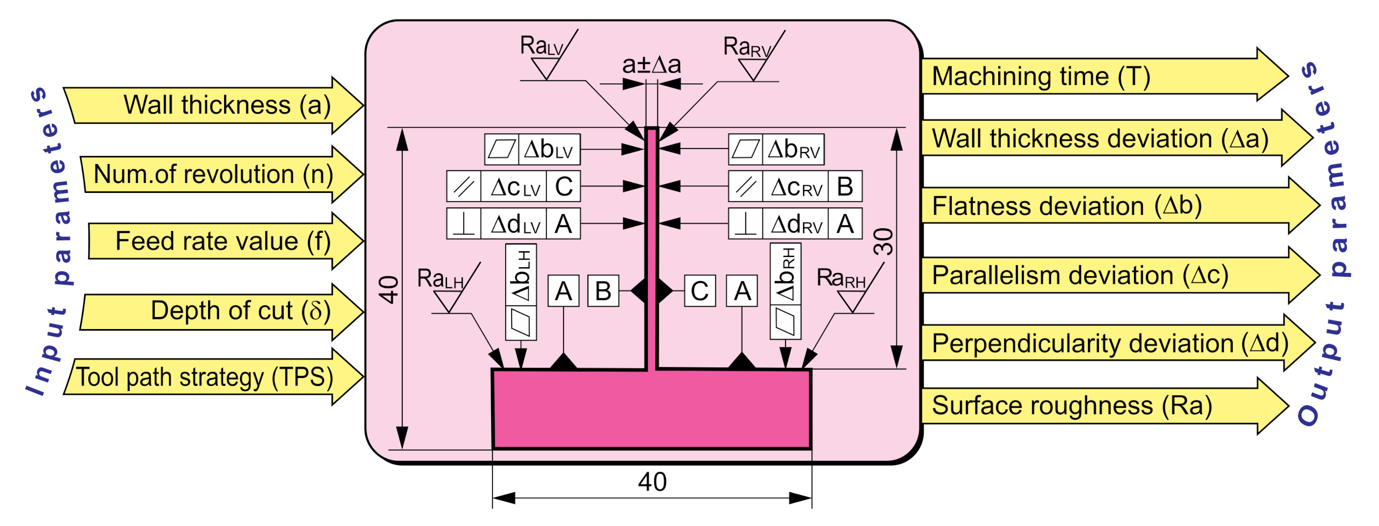
The object of this research is a linear thin-walled structure of aluminum alloy with a wall thickness of a = 0.5–1.5 mm and a wall height of 30 mm, so the parts belong to the category of moderate height-to-thickness ratio <30:1 (for 1.5 mm wall thickness) and very large height-to-thickness ratio ≥30:1 (for 0.5 mm and 1mm wall thickness).Considering that many parameters affect the process of high-speed milling of thin-walled parts, recent experimental researches were conducted to determine their limit values and level of influence on specific output parameters—optimization criteria [62]. As a result of these investigations, the following input parameters were selected: wall thickness (a), number of revolutions (n), feed rate (f), depth of cut (δ), and tool path strategy (TPS) while the output parameters were measured and calculated: machining time (T) / material removal rate (MRR), wall thickness deviation (Δa), flatness deviation (Δb), parallelism deviation (Δc), perpendicularity deviation (Δd) surface roughness (Ra), Figure 2.
The main optimization task refers to determining the optimal machining parameters of the observed thin-walled parts as an objective function by achieving high productivity, the accuracy of measures, quality of machining, the accuracy of form and surface position order of importance of the criteria. The hierarchical structure of the optimization problem consists of the following elements:
  • Objective function: Optimum machining parameter levels of the line-type thin-walled parts of aluminum alloy from the aspect of high productivity, accuracy, and quality of machining;
  • Optimization criteria: Output parameters of the machining process (MRR, Δa, Δb, Δc, Δd, and Ra);
  • Alternative solutions (alternative variants): Selected combinations-levels of input parameters of the process (a, n, f, δ, and TPS) based on the designed experimental plan.

3.2. Experimental Design

Assuming that the mathematical relations of the input parameters and performances of the process are complex and nonlinear, three levels of variations were chosen for each parameter (Table 1). When choosing the parameters’ values, literature recommendations, technical and technological limitations of the machine and tools, characteristics of the workpiece material, and previous experimental research were taken into account.
The planning of the experiment was performed using the Taguchi methodology, which is very often and efficiently applied for experimental analysis and optimization of production processes [63]. Based on the selected varying input machining parameters and the corresponding levels of variation, an experimental design matrix was made using the standard Taguchi orthogonal array L27 consisting of 27 rows (experimental trials) and 13 columns (parameter levels) where the input parameter levels are connected to columns 1, 2, 5, 9 and 12.

3.3. Realizing the Experiments

A blank material used for machining sample parts is the prismatic shape (70 mm × 40 mm × 40 mm), and the material is alloy Al7075 (AlZnMgCu1.5). This aluminum alloy has very good mechanical properties, high fatigue, and corrosion resistance, making it suitable for the machining of thin-walled structures. The chemical composition of this alloy is: Al (87.1–91.4%), Cr (0.18–0.28%), Cu (1.2–2%), Fe (≤0.5%), Mg (2.1–2.9%), Mn (≤0.3%), Si (≤0.4%), Ti (≤0.2%), Zn (5.1–6.1%). The main mechanical properties are tensile strength (560 MPa), Rp0.2 (500 MPa), yield strength (7%), hardness (150 HBW). Experimental investigations were performed on the high-speed CNC vertical milling machining center DIGMA HSC 850 (Frezal, Ruma, Serbia), using high-pressure air as a coolant during machining. The Alu-power carbide end mill cutter, manufactured by YG (Incheon, South Korea), was used for machining parts. The basic tool information is the following: diameter D = 8 mm, helix angle 30°, 2 flutes, corner radius R = 0.6 mm, flute length L1 = 10 mm, overall length L = 70 mm. Figure 3 shows the machining system used to realize the experimental machining process with the image of the machine tool’s workspace, i.e., the main spindle with the tool and the workpiece clamped in the machine fixtures.
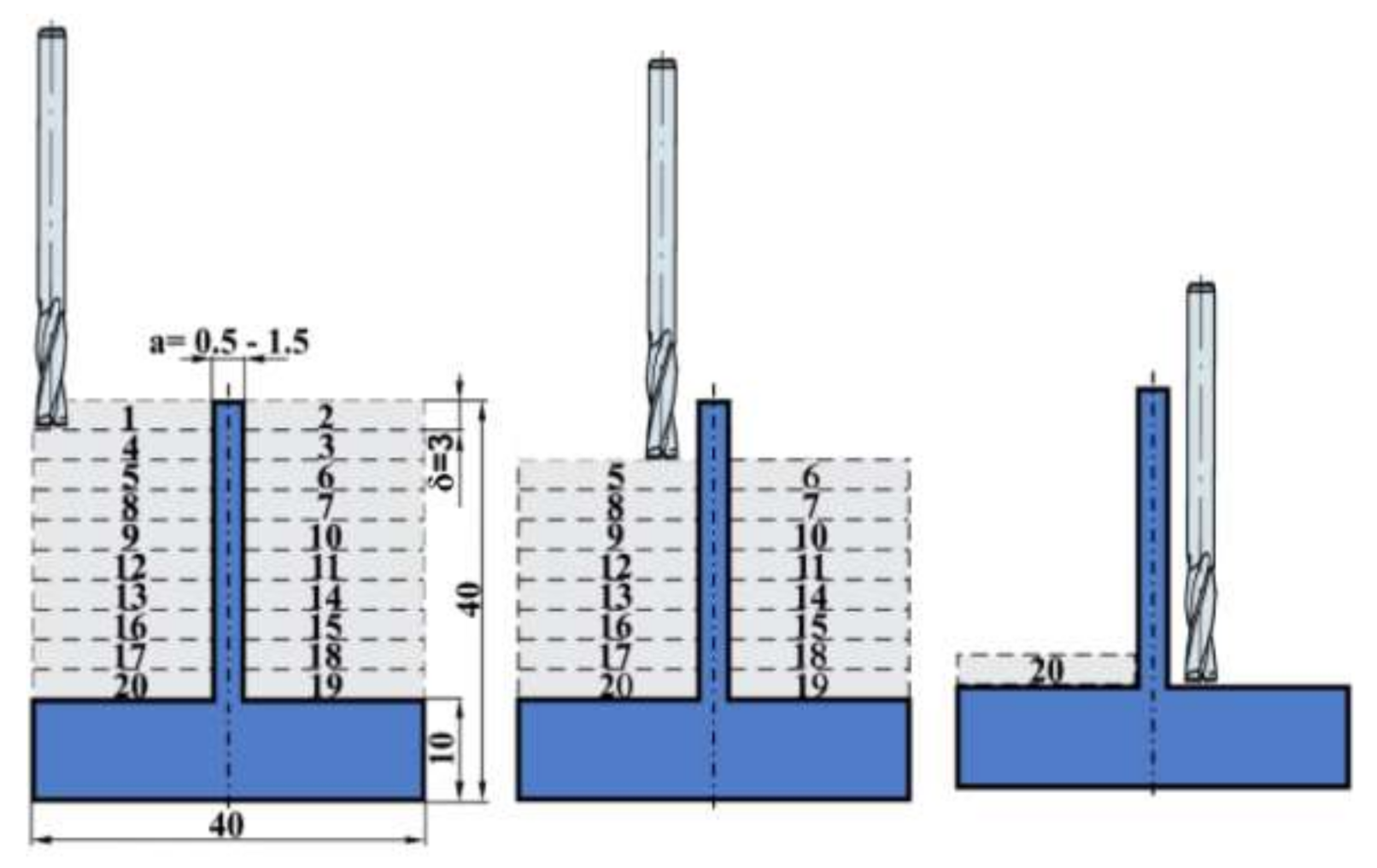
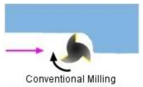
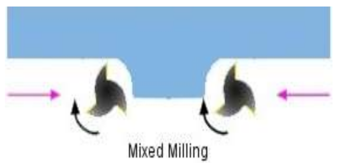
To avoid deformations in the machining process, analysis of the positive cases from the literature [9,28] and previous implementation of the experiments made it possible to choose a strategy of alternating machining of both sides of the wall. According to Figure 4, the case with the depth of cut of δ = 3 mm is represented.

3.4. Measuring the Experimental Results

As stated in the research plan, the following machining parameters were measured: machining time—T (min), wall thickness deviation—Δa (mm), flatness deviation—Δb (mm), parallelism deviation—Δc (mm), perpendicularity deviation—Δd (mm) and surface roughness—Ra (μm), as shown in Figure 2.
Based on the measured machining time for different levels of alternative input parameters, the calculation of the material removal rate (MRR) was done. It is considered an optimization criterion that shows machining productivity according to Equation (4).
MRR = V T   ( mm 3 min )
where:
  • V–the volume of removed material (mm3);
  • T–the machining time (min).
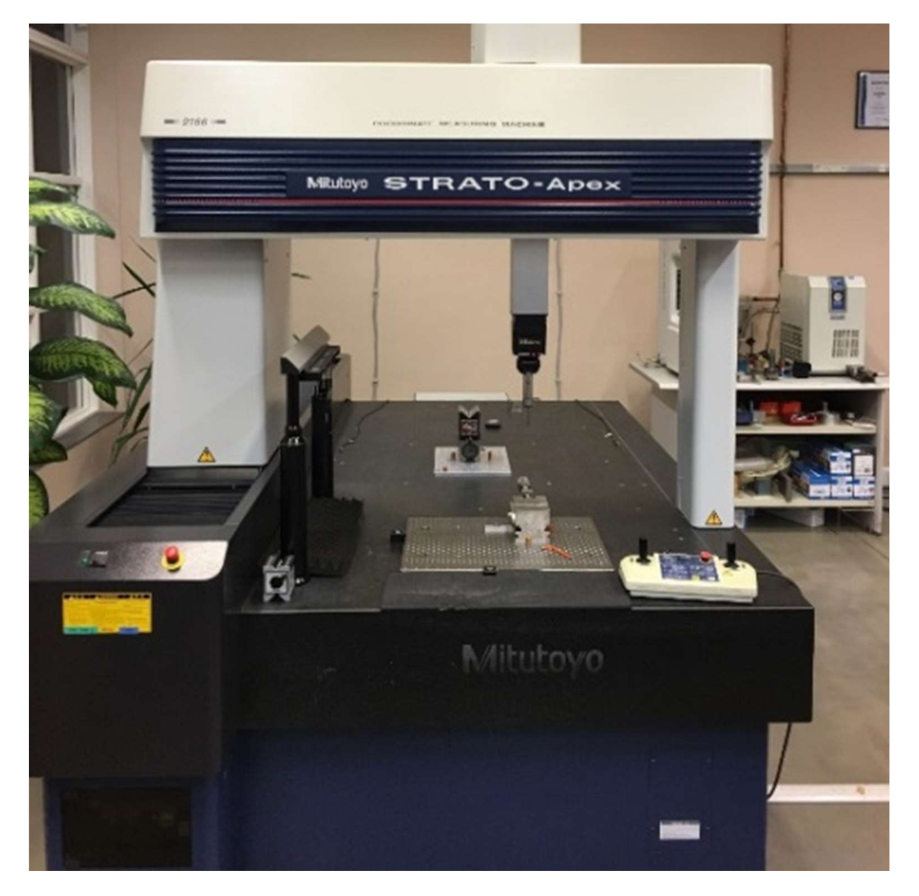
The measurement of the next four parameters (Δa, Δb, Δc, and Δd) was done using Coordinate Measuring Machines (CMM) Mitutoyo Strato—APEX 9166 Unimet, Kac, Serbia), Figure 5. Depending on the type of parameter (according to Figure 2), measurements were realized in certain places and surfaces, which is explained below for each parameter specifically. Then, the mean values of these measurements were calculated for each parameter, which represent the output values of these parameters.
The wall thickness (a) was measured in five places at equal distances along the length of the part, and then the mean deviation of the wall thickness (Δa) was calculated as the output parameter.
The flatness deviation (Δb) was measured for the left and the right side, as well as the horizontal and the vertical surface. Therefore, we have the following flatness deviations: ΔbRV—right vertical side of the wall, ΔbRH—right horizontal surface, ΔbLV—left vertical side of the wall, and ΔbLH—left horizontal side of the wall.
The parallelism deviation (Δc) was measured for the left and right side of the wall, i.e., ΔcLV—the parallelism deviation of the wall’s left vertical side, ΔcRV—the parallelism deviation of the right vertical side of the wall. The perpendicularity deviation (Δd) was measured for the left and right side of the wall, so we have ΔdLV—the perpendicularity deviation of the left vertical side of the wall, ΔdRV—the perpendicularity deviation of the right vertical side of the wall.
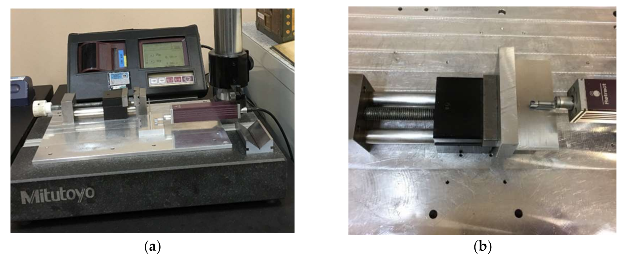
Measurement of the surface roughness was performed using the Mitutoyo SJ-301 device (Unimet, Kac, Serbia), Figure 6. Roughness was measured perpendicularly to the direction of the tool movement. Since it is a linear part, it is divided into the left and right side, so that the roughness of the left side of the horizontal and the vertical surface RaLH and RaLV, as well as the right side RaRH and RaRV were measured. Experimental plan matrices with measurement results (T, Δa, Δb, Δc, Δd, Ra) and calculations (MRR) are shown in Table 2.
A more detailed analysis of the results showed that the input parameters have different effects on the characteristics of the output results-optimization criteria, implying the need to optimize the machining parameters for thin-walled parts using MCDM methodologies.

4. Results and Discussion

4.1. Determining the Weight Coefficients of the Criteria

To determine the optimal machining parameters of the observed line-type thin-walled parts, it was necessary to define the optimization criteria correctly and then determine their weight coefficients. As a large amount of material is removed in the process of production of these parts, it is necessary to achieve high productivity and, at the same time, the best possible quality and accuracy of machining. For that purpose, the material removal rate (MRR) was chosen as the most important criterion, followed by the dimensional accuracy of the wall thickness (Δa) and the surface roughness (Ra). The corresponding hierarchical structure—pairwise comparison matrix (each criterion is compared with every other)—is presented using the following decision matrix in Table 3.
The approximation AHP method [44] consisted of four steps, was used to determine the weight coefficients—normalized eigenvectors of the criteria. The first step refers to the definition of the processed matrix—a table of comparison of all criteria where the values below the diagonal of the matrix get inverted values above the diagonal. The second step is to determine the sum of all the column elements in the table. The results of the first two steps are shown in Table 4.
In the third step, each column’s elements are divided by the sum of the values of that column, which was obtained in the previous step. In the fourth step, each row’s sum is determined, followed by the mean value of that row. The column consisting of these mean values represents the normalized eigenvector of the criterion (column Wj), i.e., the weight coefficients of the criterion Wj. The results of the third and fourth steps are given in Table 5, and the calculated values of weight coefficients are as follows: WMRR = 0.43571, WΔa = 0.15913, WRa = 0.15913, WΔb = 0.08201, WΔc = 0.08201, WΔd = 0.08201 and the sum of these values ΣWi = 1.00.
To determine the decision-maker’s consistency, the one who defines the level of errors when comparing the criteria, the calculation of the consistency ratio was performed. The consistency index CI according to Equation (5), is defined first, followed by the consistency ratio CR according to Equation (6), where the random index RI = 1.24 is adopted based on the number of criteria in the model (n = 6) [44].
CI = λ max n n 1 = 6.0147 6 6 1 = 0.0029
CR = CI RI = 0.0029 1.24 = 0.0024
The value of the consistency ratio equals CR = 0.0024 ≤ 0.1, which means that the decision-makers error when estimating the comparison of the criteria is very small, based on which we can conclude that the comparison of the criteria was performed adequately.

4.2. Applying the MCDM Methods

4.2.1. Results of Applying MCDM Methods

Table 6 shows the resulting coefficients obtained by applying 14 MCDM methods based on which the ranking of alternative levels of the machining parameters for milling of thin-walled parts was performed. The designations and names of these coefficients for all applied MCDM methods are given below: GRA (GRG—gray relational grade), AHP (Fi—composite normalized vector), MOORA (Yi—normalized assessment value of alternatives, TOPSIS (CCo—relative closeness to the “ideal” solution), ROV (Ui—mean value of the utility function of alternatives), COPRAS (Uj%—degree of utility alternatives), ARAS (Ui%—degree of utility alternatives), WASPAS (Qj—overall relative importance of the alternative), VIKOR (Qi—minimum distance from “ideal“ solutions), OCRA (Pi—overall performance rating), EDAS (Si—values of appraisal scores), MABAC (Si—values of criteria function of alternatives), SAW (Si—overall ranking index of i-th alternative) and SPW (Si—overall ranking index of i-th alternative).

4.2.2. Integrative Multi-Criteria Ranking of the Alternative Levels of Machining Parameters

Based on the results from Table 6, which refer to the individual evaluation and ranking of alternative levels of high-speed machining process parameters based on fourteen different MCDM methods, a comprehensive comparison and ranking of twenty-seven levels of parameters according to the experiment plan was performed using the integrated assessment methodology. To obtain a comprehensive final ranking of the machining parameter levels based on the results of applying the MCDM methods, the agreement of the obtained values of the correlation ratios with the set limit values was tested.
Table 7 provides an overview of the ranks of alternative levels, values of standard deviation by levels (σi), while the lower part of the table gives the following values: maximum standard deviation (σmax), average standard deviation (σav), Kendall’s rank correlation coefficient (W), and the average Spearman rank correlation coefficient (R). Table 8 shows the values of Spearman’s correlation coefficients of the ranks of alternative parameter levels of all applied MCDM methods by pairs.
After the first iteration, it was stated that the results obtained by applying these 14 MCDM methods could not be used for integrative ranking of the alternative parameter levels because the limit values of the first given criterion are not met (0.9 ≤ Ri ≤1), i.e., there are several combinations of methods where Spearman’s rank correlation coefficient Ri is less than the limit value of 0.9.
Since the set criteria were not met within the first iteration, it was necessary to approach the second iteration, which is presented below with the corresponding results.

Second Iteration

After analyzing the results in Table 8, it was concluded that there is a group of MCDM methods that meet all the criteria which are proven through the introduction of the second iteration. The second iteration includes the integrated application of the following five methods: MOORA, ROV, EDAS, MABAC, and SPW.
The results of comparing the ranks of the alternative levels of parameters are given in Table 9, and the values of Spearman’s rank correlation coefficients are presented in Table 10.
Based on the obtained results shown in Table 9 and Table 10, it can be concluded that for the combination of the MCDM methods MOORA, ROV, EDAS, MABAC, and SPW:
  • The first criterion is met—the Spearman’s rank correlation coefficient is for all combinations of methods within the limit value 0.9 ≤ Ri ≤ 1 (Rmin = 0.9115),
  • The second criterion is met—Kendall’s rank correlation coefficient is in the range of 0.9 ≤ W (W = 0.9728),
  • The third criterion is met—average Spearman rank correlation coefficient is in the range of 0.9 ≤ R (R = 0.9708) and
  • The fourth criterion is met—the average standard deviation is within the limit value σav ≤ 1.5 (σav = 1.0729)
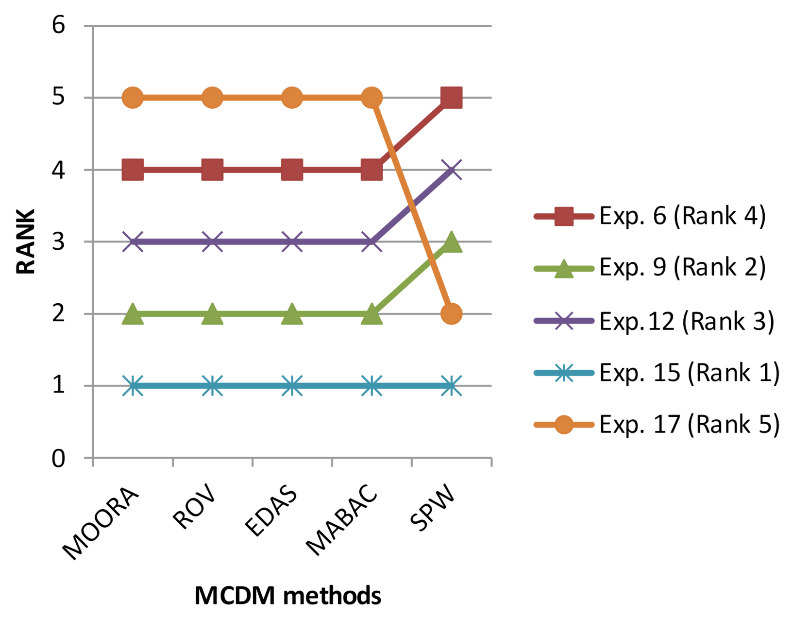
Since all the correlation criteria for the integrative application of MCDM methods are met, the optimal rank of the alternative levels of process parameters is given in Table 9. Table 11 shows the five best-ranked levels with values of machining parameters (a, n, f, δ, and TPS) and the values of the obtained optimization criteria (MRR, Δa, Δb, Δc, Δd, and Ra). Figure 7 presents the ranking chart of the top 5 alternative experiments according to the selected MCDM methods.

5. Conclusions

In this study, the machining parameters for milling of line-type thin-walled parts made of aluminum alloy Al 7075 were analyzed. The influence of wall thickness (a), number of revolutions (n), feed rate (f), depth of cut (δ), and tool path strategy (TPS) was examined on machining time (T)/material removal rate (MRR), wall thickness deviation (Δa), surface flatness deviation (Δb), surface parallelism deviation (Δc), surface perpendicularity deviation (Δd) and surface roughness (Ra), all of them representing the optimization criteria.
Considering the characteristics of the process of high-speed milling of thin-walled parts, a comparison of optimization criteria using the AHP method was made, where the highest weight coefficient was obtained by the material removal rate (MRR), as a productivity opponent WMRR = 0.43571, then weight coefficients of the wall thickness accuracy and surface roughness WΔa = 0.15913, WRa = 0.15913, and finally the accuracy of form and accuracy of surface position WΔb = 0.08201, WΔc = 0.08201 and WΔd = 0.08201. Twenty-seven experiments were conducted using the standard Taguchi orthogonal sequence L27, and multi-criteria optimization was performed using 14 MCDM methods (GRA, AHP, MOORA, TOPSIS, ROV, COPRAS, ARAS, WASPAS, VIKOR, OCRA, EDAS, MABAC, SAW and SPW) According to this, the optimal alternative levels of input parameters for the defined objective function and their ranking were obtained.
Afterward, the obtained results were compared using correlation analysis based on Spearman’s and Kendall’s rank correlation coefficients and the standard deviation of the ranks of the alternative levels. At the output, the integrative decision on selecting the optimal level of high-speed machining parameters based on 5 MCDM methods (MOORA, ROV, EDAS, MABAC and SPW) that met the limits of correlation coefficients was made. The optimum machining parameter level is experiment No.15 with the following varying input parameters a = 1 mm, n = 12,000 rpm, f = 2400 mm/min, δ = 2 mm, TPS 3 and the output machining parameters as the optimization criteria: MRR=14,980.790 mm3/min, Δa = 0.0260 mm, Δb = 0.03650 mm, Δc = 0.0905 mm, Δd = 0.1510 mm and Ra = 1.0050 μm.
Author Contributions

Conceptualization, D.L. and J.V.; methodology D.L., M.M. and R.C.; experimentation and measurement D.L., J.V. and A.A.; software D.L. and M.M.; validation D.L. and M.D.; writing—original draft preparation D.L. and J.V.; writing—review and editing, M.M. and M.D.; supervision R.C. and A.A. All authors have read and agreed to the published version of the manuscript.

Funding

This research received no external funding.

Acknowledgments

This paper is part of a research on the project “Application of smart manufacturing methods in Industry 4.0”, No. 142-451-3173/2020, Provincial Secretariat for Higher Education and Scientific Research of the Autonomous Province of Vojvodina and on the project “Innovative scientific and artistic research from the FTS (activity) domain”, No. 451-03-68/2020-14/200156, Ministry of Education, Science and Technological Development of the Republic of Serbia.

Conflicts of Interest

The authors declare no conflict of interest.

References

  1. Hirsch, J.; Al-Samman, T. Superior light metals by texture engineering: Optimized aluminum and magnesium alloys for automotive applications. Acta Mater. 2013, 61, 818–843. [Google Scholar] [CrossRef]
  2. Bolar, G. Numerical and Experimental Studies on Thin-Wall Machining of Aerospace Grade Aluminum Alloy. Ph.D. Thesis, Indian Institute of Technology Guwahati, Assam, India, 2017. Available online: http://gyan.iitg.ernet.in/handle/123456789/1298 (accessed on 10 June 2020).
  3. Stojanovic, B.; Ivanovic, L. Application of aluminium hybrid composites in automotive industry. Teh. Vjes. 2015, 22, 247–251. [Google Scholar] [CrossRef] [Green Version]
  4. Izamshah, R.A.; Mo, J.P.T.; Ding, S. Hybrid deflection prediction on machining thin-wall monolithic aerospace components. Proc. Inst. Mech. Eng. Part B J. Eng. Manuf. 2011, 226, 592–605. [Google Scholar] [CrossRef]
  5. Del Sol, I.; Rivero, A.; López de Lacalle, L.N.; Gamez, A.J. Thin-wall machining of light alloys: A review of models and industrial approaches. Materials 2019, 12, 2012. [Google Scholar] [CrossRef] [PubMed] [Green Version]
  6. Huang, X.; Sun, J.; Li, J. Effect of initial residual stress and machining-induced residual stress on the deformation of aluminium alloy plate. Stroj. Vestn. J. Mech. E. 2015, 61, 131–137. [Google Scholar] [CrossRef] [Green Version]
  7. Zhou, X.; Zhang, D.; Luo, M.; Wu, B. Toolpath dependent chatter suppression in multi-axis milling of hollow fan blades with ball-end cutter. Int. J. Adv. Manuf. Technol. 2014, 72, 643–651. [Google Scholar] [CrossRef]
  8. Jiang, X.; Zhu, Y.; Zhang, Z.; Guo, M.; Ding, Z. Investigation of residual impact stress and its effects on the precision during milling of the thin-walled part. Int. J. Adv. Manuf. Technol. 2018, 97, 877–892. [Google Scholar] [CrossRef]
  9. Borojević, S.; Lukić, D.; Milošević, M.; Vukman, J.; Kramar, D. Optimization of process parameters for machining of Al 7075 thin-walled structures. Adv. Prod. Manag. 2018, 13, 125–135. [Google Scholar] [CrossRef]
  10. Zhang, D.; Gao, K.; Zhou, T. Discussion on NC machining process of thin walled parts technical measures. Appl. Mech. Mater. 2015, 701–702, 864–868. [Google Scholar] [CrossRef]
  11. Bing, D.; Yu, G.-B.; Guan, Y.-Q.; Shao, J.-P.; Guan, Y.-Q.; Wu, X.-M.; Liu, Y.-X. Machining Surface Quality Analysis of Aluminum Alloy Thin-Walled Parts in Aerospace. Int. J. Secur. Appl. 2015, 9, 201–208. [Google Scholar] [CrossRef]
  12. Cica, D.; Borojevic, S.; Jotic, G.; Sredanovic, B.; Tesic, S. Multiple performance characteristics optimization in end milling of thin-walled parts using desirability function. Trans. Can. Soc. Mech. Eng. 2019, 44, 84–94. [Google Scholar] [CrossRef]
  13. Bolar, G.; Das, A.; Joshi, S.N. Measurement and analysis of cutting force and product surface quality during end-milling of thin-wall components. Meas. J. Int. Meas. Confed. 2018, 121, 190–204. [Google Scholar] [CrossRef]
  14. Antic, A.; Kozak, D.; Kosec, B.; Simunovic, G.; Saric, T.; Kovacevic, D.; Čep, R. Influence of tool wear on the mechanism of chips segmentation and tool vibration. Teh. Vjes. 2013, 23, 105–112. Available online: https://hrcak.srce.hr/97486 (accessed on 5 June 2020).
  15. Vukman, J.; Lukic, D.; Borojevic, S.; Rodic, D.; Milosevic, M. Application of Fuzzy Logic in the Analysis of Surface Roughness of Thin-Walled Aluminum Parts. Int. J. Precis. Eng. Manuf. 2020, 21, 91–102. [Google Scholar] [CrossRef]
  16. Aijun, T.; Zhanqiang, L. Deformations of thin-walled plate due to static end milling force. J. Mater. Process. Technol. 2008, 206, 345–351. [Google Scholar] [CrossRef]
  17. Ning, H.; Zhigang, W.; Chengyu, J.; Bing, Z. Finite element method analysis and control stratagem for machining deformation of thin-walled components. J. Mater. Process. Technol. 2003, 139, 332–336. [Google Scholar] [CrossRef]
  18. Yan, Q.; Luo, M.; Tang, K. Multi-axis variable depth-of-cut machining of thin-walled workpieces based on the workpiece deflection constraint. Comput. Aided Design. 2018, 100, 14–29. [Google Scholar] [CrossRef]
  19. Rai, J.K.; Xirouchakis, P. Finite element method based machining simulation environment for analyzing part errors induced during milling of thin-walled components. Int. J. Mach. Tools Manuf. 2008, 48, 629–643. [Google Scholar] [CrossRef]
  20. Wang, L.; Si, H. Machining deformation prediction of thin-walled workpieces in five-axis flank milling. Int. J. Adv. Manuf. Technol. 2018, 97, 4179–4193. [Google Scholar] [CrossRef]
  21. Wang, L.; Huang, H.; West, R.W.; Li, H.; Du, J. A model of deformation of thin-wall surface parts during milling machining process. J. Cent. South Univ. 2018, 25, 1107–1115. [Google Scholar] [CrossRef]
  22. Sapthagiri, S.; Rao, K.J. Optimization of Machining Parameters with Minimum Distortion of a Thin Wall and Thin Floor Avionic Component. Int. J. Emerg. Technol. Adv. Eng. 2016, 6, 154–159. Available online: https://www.ijetae.com/files/Volume6Issue7/IJETAE_0716_23.pdf (accessed on 25 May 2020).
  23. Savkovic, B.; Kovac, P.; Stoic, A.; Dudic, B. Optimization of Machining Parameters Using the Taguchi and ANOVA Analysis in the Face Milling of Aluminum Alloys AL7075. Teh. Vjes. 2020, 27, 1221–1228. [Google Scholar] [CrossRef]
  24. Sridhar, G.; Babu, P.R. Effect of material removal rate on machining distortion of thin-wall thin-floor components. Mater. Today-Proc. 2018, 5, 27018–27027. [Google Scholar] [CrossRef]
  25. Qu, S.; Zhao, J.; Wang, T. Experimental study and machining parameter optimization in milling thin-walled plates based on NSGA-II. Int. J. Adv. Manuf. Technol. 2017, 89, 2399–2409. [Google Scholar] [CrossRef]
  26. Bolar, G.; Mekonen, M.; Das, A.; Joshi, S.N. Experimental Investigation on Surface Quality and Dimensional Accuracy during Curvilinear Thin-Wall Machining. Mater. Today-Proc. 2018, 5, 6461–6469. [Google Scholar] [CrossRef]
  27. Shamsuddin, K.A.; Ab-Kadir, A.R.; Osman, M.H. A Comparison of Milling Cutting Path Strategies for Thin Walled Aluminium Alloys Fabrication. Int. J. Eng. Sci. (IJES) 2013, 2, 1–8. Available online: http://www.theijes.com/papers/v2-i3/A0230108.pdf (accessed on 27 May 2020).
  28. Popma, M. Computer Aided Process Planning for High-Speed Milling of Thin Walled Parts. Ph.D. Thesis, University of Twente, Enschede, The Netherlands, 2010. [Google Scholar] [CrossRef] [Green Version]
  29. Olvera, D.; Urbikain, G.; Elías-Zuñiga, A.; López de Lacalle, L.N. Improving Stability Prediction in Peripheral Milling of Al7075T6. Appl. Sci. 2018, 8, 1316. [Google Scholar] [CrossRef] [Green Version]
  30. Gong, H.; Sun, Y.; Liu, Y.; Wu, Y.; He, Y.; Sun, X.; Zhang, M. Effect of Vibration Stress Relief on the Shape Stability of Aluminum Alloy 7075 Thin-Walled Parts. Metals 2019, 9, 27. [Google Scholar] [CrossRef] [Green Version]
  31. Wimmer, S.; Zaeh, M.F. The Prediction of Surface Error Characteristics in the Peripheral Milling of Thin-Walled Structures. J. Manuf. Mater. Process. 2018, 2, 13. [Google Scholar] [CrossRef] [Green Version]
  32. Köksalan, M.; Wallenius, J.; Zionts, S. Multiple Criteria Decision Making: From Early History to the 21st Century; World Scientific: Singapore, 2011. [Google Scholar]
  33. Chakraborty, S. Applications of the MOORA method for decision making in manufacturing environment. Int. J. Adv. Manuf. Technol. 2011, 54, 1155–1166. [Google Scholar] [CrossRef]
  34. Triantaphyllou, E. Multi-Criteria Decision Making: A Comparative Study; Kluwer Academic Publishers (now Springer): Dordrecht, The Netherlands, 2000. [Google Scholar]
  35. Lukic, D.; Milosevic, M.; Antic, A.; Borojevic, S.; Ficko, M. Multi-criteria selection of manufacturing processes in the conceptual process planning. Adv. Prod. Manag. 2017, 12, 151–162. [Google Scholar] [CrossRef] [Green Version]
  36. Tzeng, G.H.; Huang, J.J. Multiple Attribute Decision Making: Methods and Applications; CRC Press: Boca Raton, FL, USA, 2011. [Google Scholar]
  37. Vinogradova, I. Multi-attribute decision-making methods as a part of mathematical optimization. Mathematics 2019, 7, 915. [Google Scholar] [CrossRef] [Green Version]
  38. Madic, M.; Nedic, B.; Radovanovic, M. Poslovno i Inženjersko Odlučivanje Primenom Metoda Višekriterijumskog Odlučivanja; Fakultet Inzenjerskih Nauka, Univerzitet u Kragujevcu: Kragujevac, Serbia, 2015. (In Serbian) [Google Scholar]
  39. Zavadskas, E.K.; Turskis, Z.; Kildiene, S. State of art surveys of overviews on MCDM/MADM methods. Technol. Econ. Dev. Econ. 2014, 20, 165–179. [Google Scholar] [CrossRef] [Green Version]
  40. Ishizaka, A.; Nemery, P. Multi-Criteria Decision Analysis: Methods and Software; John Willey & Sons: Hoboken, NJ, USA, 2013. [Google Scholar]
  41. Marinkovic, G.; Ninkov, T.; Trifkovic, M.; Nestorovic, Z.; Pejicic, G. On the land consolidation projects and cadastral municipalities ranking. Teh. Vjes. 2016, 23, 1147–1153. [Google Scholar] [CrossRef] [Green Version]
  42. Jahan, A.; Edwards, K.L.; Bahraminasab, M. Multi-criteria Decision Analysis for Supporting the Selection of Engineering Materials in Product Design, 2nd ed.; Elsevier Science: Amsterdam, The Netherlands, 2016. [Google Scholar] [CrossRef]
  43. Deng, J.L. Control problems of grey systems. Syst. Control Lett. 1982, 1, 288–294. [Google Scholar] [CrossRef]
  44. Saaty, T.L. The Analytic Hierarchy Process: Planning, Priority Setting, Resource Allocation; McGraw-Hill: New York, NY, USA, 1990. [Google Scholar]
  45. Brauers, W.K. Optimization Methods for a Stakeholder Society, a Revolution in Economic Thinking by Multi-Objective Optimization; Springer US: New York, NY, USA, 2004. [Google Scholar]
  46. Hwang, C.L.; Yoon, K. Multiple Attribute Decision Making Methods and Applications; Springer: Berlin, Germany, 1981. [Google Scholar]
  47. Yakowitz, D.S.; Lane, L.J.; Szidarovszky, F. Multi-attribute decision making: Dominance with respect to an importance order of the attributes. Appl. Math. Comp. 1993, 54, 167–181. [Google Scholar] [CrossRef]
  48. Zavadskas, E.K.; Kaklauskas, A.; Sarka, V. The new method of multicriteria complex proportional assessment of projects. Technol. Econ. Dev. Econ. 1994, 1, 131–139. [Google Scholar]
  49. Zavadskas, E.K.; Turskis, Z. A new Additive Ratio Assessment (ARAS) method in multicriteria decision-making. Technol. Econ. Dev. Econ. 2010, 16, 159–172. [Google Scholar] [CrossRef]
  50. Zavadskas, E.K.; Turskis, J.; Antucheviciene, A.; Zakarevicius, A. Optimization of weighted aggregated sum product assessment. Elektron. Elektrotech. 2012, 122, 3–6. [Google Scholar] [CrossRef]
  51. Opricovic, S.; Tzeng, G.H. Extended VIKOR method in comparison with outranking methods. Eur. J. Oper. Res. 2007, 178, 514–529. [Google Scholar] [CrossRef]
  52. Parkan, C.; Wu, M.L. On the equivalence of operational performance measurement and multi-attribute decision making. Int. J. Prod. Res. 1997, 35, 2963–2988. [Google Scholar] [CrossRef]
  53. Keshavarz-Ghorabaee, M.; Zavadskas, E.K.; Olfat, L.; Turskis, Z. Multi-criteria inventory classification using a new method of evaluation based on distance from average solution (EDAS). Informatica 2015, 26, 435–451. [Google Scholar] [CrossRef]
  54. Keshavarz-Ghorabaee, M.; Amiri, M.; Zavadskas, E.K.; Turskis, Z.; Antucheviciene, J. A Dynamic Fuzzy Approach Based on the EDAS Method for Multi-Criteria Subcontractor Evaluation. Information 2018, 9, 68. [Google Scholar] [CrossRef] [Green Version]
  55. Pamucar, D.; Cirovic, G. The selection of transport and handling resources in logistics centers using Multi-Attributive Border Approximation area Comparison (MABAC). Expert Syst. Appl. 2015, 42, 3016–3028. [Google Scholar] [CrossRef]
  56. MacCrimmon, K.R. Decision Making Among Multiple-Attribute Alternatives: A Survey and Consolidated Approach; The Rand Corporation: Santa Monica, CA, USA, 1968; Available online: https://www.rand.org/pubs/research_memoranda/RM4823.html (accessed on 25 June 2020).
  57. Opricovic, S.; Tzeng, G.H. Compromise solution by MCDM methods: A comparative analysis of VIKOR and TOPSIS. Eur. J. Oper. Res. 2004, 156, 445–455. [Google Scholar] [CrossRef]
  58. Tripathy, S.; Tripathy, D.K. Multi-attribute optimization of machining process parameters in powder mixed electro-discharge machining using TOPSIS and grey relational analysis. Eng. Sci. Technol. Int. J. 2016, 19, 62–70. [Google Scholar] [CrossRef] [Green Version]
  59. Moradian, M.; Modanloo, V.; Aghaiee, S. Comparative analysis of multi criteria decision making techniques for material selection of brake booster valve body. J. Traffic Transp. Eng. 2019, 6, 526–534. [Google Scholar] [CrossRef]
  60. King, S.D.; Rosopa, P.J.; Minium, E.W. Statistical Reasoning in the Behavioral Sciences, 7th ed.; Willey; USA John Wiley & Sons, Inc.: Hoboken, NJ, USA, 2018. [Google Scholar]
  61. Howell, D. Statistical Methods for Psychology; Wadsworth, Cengage Learning: Boston, MA, USA, 2013. [Google Scholar]
  62. Vukman, J.; Lukic, D.; Borojevic, S.; Milosevic, M.; Kramar, D. Experimental Research of The Influence of High-Speed Machining Parameters on Time and Surface Roughness of Thin-Walled Parts. In Proceedings of the 13th International Scientific Conference “Flexible Technologies”—MMA, Novi Sad, Serbia, 28–29 September 2018; Faculty of Technical Sciences: Novi Sad, Serbia, 2018; pp. 227–232. [Google Scholar]
  63. Taguchi, G.; Chowdhury, S.; Wu, Y. Taguchi’s Quality Engineering Handbook; John Wiley & Sons, Inc.: Hoboken, NJ, USA, 2005. [Google Scholar]
Figure 1. Influential machining parameters for thin-walled parts.
Metals 10 01570 g001
Figure 2. The optimization tasks (unit: mm).
Metals 10 01570 g002
Figure 3. Workspace of the machine tool.
Metals 10 01570 g003
Figure 4. Selected machining passes sequence for the machining of thin-walled parts.
Metals 10 01570 g004
Figure 5. Coordinate Measuring Machines (CMM) Mitutoyo Strato—APEX 9166.
Metals 10 01570 g005
Figure 6. Measurement of the surface roughness (Ra) using Mitutoyo SJ-301 device: (a) Horizontal surfaces; (b) Vertical surfaces.
Metals 10 01570 g006
Figure 7. Ranking chart of the 5 best alternative experiments for the selected MCDM methods.
Metals 10 01570 g007
Table 1. Input parameters and levels of variation.
ParameterUnitLevel
Wall thickness (a)mm0.511.5
Number of revolutions (n)rpm600012,00024,000
Feed rate (f)mm/min60012002400
Depth of cut (δ)mm123
Tool path strategy (TPS)—Cimatron-Path 1-climb
Metals 10 01570 i001
Path 2-conventional
Metals 10 01570 i002
Path 3-mixed
Metals 10 01570 i003
Table 2. Experimental design and the results of measurements/calculations.
No.Input ParametersOutput Parameters—Optimization Criteria
anfδTPSTMRRΔaΔbΔcΔdRa
mmrpmmm/minmm-hh:mm:ssmm3/minmmmmmmmmμm
10.560006001100:36:402262.2520.04200.038750.06900.08400.2500
20.5600012002200:11:307213.0430.02400.127250.24150.38301.3100
30.5600024003300:19:294257.5580.02600.049250.08450.12200.8300
40.512,0006002300:21:063931.2800.01600.048500.10350.11600.8425
50.512,00012003100:42:101967.1780.01600.034750.06450.09250.3375
60.512,00024001200:09:168951.1170.02200.064750.10850.10150.8600
70.524,0006003200:47:161754.9240.01200.041750.11600.13350.4100
80.524,00012001300:17:174799.5140.02600.033750.08750.11950.3950
90.524,00024002100:08:379626.3200.03800.039750.06850.10000.2925
101.060006002200:22:333631.9290.06000.057500.13550.12501.5325
111.0600012003300:29:032819.2770.03800.025250.13550.17300.5800
121.0600024001100:11:237194.9400.01000.020500.11350.11700.5100
131.012,0006003101:03:541281.6900.00800.011500.08900.09400.1375
141.012,00012001200:17:464609.6700.05600.023750.06000.10900.6325
151.012,00024002300:05:2814,980.7900.02600.036500.09050.15101.0050
161.024,0006001300:28:032919.7860.04200.016500.13050.11950.1850
171.024,00012002100:12:006825.0000.02800.015500.07900.14050.1925
181.024,00024003200:23:003560.8700.03600.024750.09600.10600.3050
191.560006003300:58:061391.5660.02400.261750.09250.23250.2575
201.5600012001100:17:494537.8010.01400.273000.21150.32900.3825
211.5600024002200:06:1313,004.6600.06600.316750.31650.47151.9800
221.512,0006001200:31:232576.2360.04000.288750.21800.33351.1600
231.512,00012002300:11:177165.6470.01600.298500.27900.45901.3275
241.512,00024003100:21:593677.8420.01000.271000.17900.27250.4075
251.524,0006002100:21:333751.7400.01000.271000.34800.32150.1500
261.524,00012003200:35:272280.6770.01200.278750.26150.42450.2725
271.524,00024001300:08:189740,9640.01200.274750.21000.34000.5050
Table 3. Hierarchical structure of the pairwise criteria comparison.
ParametersMRRΔaΔbΔcΔdRa
MRR135553
Δa-12221
Δb--1111/2
Δc---111/2
Δd----11/2
Ra-----1
Table 4. Steps 1 and 2 of the approximation Analytic Hierarchy Process (AHP) methodology for determining weight coefficients.
ParametersMRRΔaΔbΔcΔdRa
MRR1.00003.00005.00005.00005.00003.0000
Δa0.33331.00002.00002.00002.00001.0000
Δb0.20000.50001.00001.00001.00000.5000
Δc0.20000.50001.00001.00001.00000.5000
Δd0.20000.50001.00001.00001.00000.5000
Ra0.33331.00002.00002.00002.00001.0000
Sum2.26676.500012.000012.000012.00006.5000
Table 5. Steps 3 and 4 of the approximation Analytic Hierarchy Process (AHP) methodology for determining weight coefficients.
ParametersMRRΔaΔbΔcΔdRaSumWjλi
MRR0.44120.46150.41670.41670.41670.46152.61430.435716.0147
Δa0.14710.15380.16670.16670.16670.15380.95480.159136.0051
Δb0.08820.07690.08330.08330.08330.07690.49210.082016.0028
Δc0.08820.07690.08330.08330.08330.07690.49210.082016.0028
Δd0.08820.07690.08330.08330.08330.07690.49210.082016.0028
Ra0.14710.15380.16670.16670.16670.15380.95480.159136.0051
-------Σ = 1.0000λmax = 6.0147
Table 6. Resulting coefficients of applying multi-criteria decision making (MCDM) methods and the rank of the alternative levels.
No. Exp.MCDM Method
GRAAHPMOORATOPSISROVCOPRASARASWASPASVIKOROCRAEDASMABACSAWSPW
GRGRankFiRankYiRankCCoRankUiRankUj%RankUi%RankQjRankQiRankPiRankSiRankSiRankSiRankSiRank
10.576430.032316−0.0360170.3293230.2413160.47861951.1608160.3178160.7653223.9233120.445316−0.0052160.3613150.274219
20.2316250.032317−0.0374190.447280.2309190.52601451.1481170.3006210.564882.4153220.434018−0.0261190.3253220.275918
30.3898160.030621−0.0212120.3603160.2623120.51231548.4040210.3171170.6418113.6446140.4940120.0368120.3330190.301314
40.4056140.031719−0.0176100.3617150.2683100.52991350.1936190.3282150.6459123.7772130.5046100.0488100.3463160.310113
50.598720.033714−0.0178110.3465190.268890.6426953.2646140.3341140.7317184.333960.5044110.049790.3795120.288715
60.4126130.045180.042040.592550.337840.7384671.294280.442560.306734.0542110.705640.187840.471470.41365
70.4446120.029722−0.0277130.3374210.2551130.55641146.9321220.2905220.7642214.147590.4707130.0225130.3271210.254021
80.4508110.0364110.004470.4126100.291670.63721057.4954110.376980.568194.311470.584170.095470.3858110.36807
90.547850.053230.063820.642420.360320.8387384.157030.527720.238724,714950.783220.232820.552730.50283
100.2827230.023026−0.0958260.2392260.1667260.34192636.3544260.2303250.8316241.9776240.237426−0.1544260.2490260.211625
110.3517170.025724−0.0483210.3112250.2243200.42002340.6486240.2572230.7696233.6094150.405821−0.0392200.2667240.247823
120.538160.051050.046530.531760.345030.8320480.614050.514540.371854.847720.724530.202330.527750.50134
130.752210.05392−0.011580.3569180.277080.9177285.277120.447450.7480204.791930.525780.066180.566120.32869
140.521670.035112-0.0325150.3594170.2436150.48141855.4603120.3470120.6580133.5684160.459615−0.0007150.3763130.317611
150.4750100.063210.114410.835810.423111.00001100.00010.569310.000014.725940.947810.358310.632310.50631
160.493780.037910−0.0306140.3464200.2450140.49571759.9038100.3520100.7300174.1193100.4668140.0023140.3860100.318010
170.559540.052540.038550.512570.331350.7951582.997740.517030.411564.866510.701050.174750.529840.50432
180.478190.034513−0.017590.3639140.2635110.54781254.5216130.3469130.6704144.170180.510090.0392110.3650140.32878
190.3448190.023925−0.0634240.3122240.2028230.35262437.7680250.2251260.8691262.4285210.340224−0.0822230.2649250.185426
200.3086220.031420−0.0348160.3917110.2325180.46462049.6901200.3075190.6800152.5104200.439017−0.0228180.3278200.287316
210.2103260.04567−0.0576230.598640.1909240.7290772.064170.3477110.510870.0000270.348923−0.1060240.441780.253722
220.1829270.016127−0.1191270.2094270.1285270.27832725.4879270.1650270.9429270.7382260.148527−0.2307270.1721270.157927
230.2370240.033615−0.0556220.441090.2039220.50061653.0725150.3031200.6126101.2713250.361622−0.0799220.3403180.265920
240.3477180.032218−0.0365180.3693130.2341170.44942150.9218180.3131180.7152162.5758190.431619−0.0196170.3442170.282117
250.4016150.04079−0.0445200.3823120.2171210.43112264.296290.366590.7407192.6001180.407020−0.0535210.421390.311612
260.3297210.027523−0.0703250.3310220.1861250.34442543.4779230.2562240.8583252.2118230.317025−0.1156250.2911230.221224
270.3345200.047460.031360.636730.311560.7059874.984860.435970.316542.9813170.660260.135260.479860.39196
Table 7. Results of comparing the ranks of the alternative parameter levels of the applied MCDM methods.
No. Exp.GRAAHPMOORATOPSISROVCOPRASARASWASPASVIKOROCRAEDASMABACSAWSPWAverage Value of RanksFinal
Rank of Alternative
σi—Stand Deviation
131617231619161622121616151916.33154.721
22517198191417218221819221816.83174.877
3162112161215211711141212191414.06143.371
4141910151013191512131010161312.67113.082
52141119991414186119121512.00104.551
613845468631144755.6752.894
712221321131122222191313212116.67165.014
8111171071011897771178.3971.805
9532223322522332.6121.051
10232626262626262524242626262524.94261.008
11172421252023242323152120242320.89232.872
12653634545233544.0031.231
1312818822520388298.7285.908
1471215171518121213161515131113.61132.818
151011111111411111.6712.476
1681014201417101017101414101013.06123.539
17445755436155424.4441.541
189139141112131314891114811.1792.301
19192524242324252626212423252623.83251.979
20222016111820201915201718201617.50202.828
21267234247711727232482217.72218.939
22272727272727272727262727272726.61270.267
2324152292216152010252222182019.00224.957
24181818131721181816191917171717.17181.785
2515920122122991918202191217.17185.229
26212325222525232425232525232423.78241.311
2720663686741766667.2864.781
Maximum standard deviation σmax =8.939
Average standard deviation σav =3.227
Kendall’s rank correlation coefficient W =0.786
Average Spearman rank correlation coefficient R =0.770
Table 8. Spearman’s rank correlation coefficients of the applied MCDM methods.
MethodsGRAAHPMOORATOPSISROVCOPRASARASWASPASVIKOROCRAEDASMABACSAWSPW
GRA10.55430.68620.07390.71180.54270.55430.63430.17520.89930.69350.71180.62450.6368
AHP-10.74730.76430.72950.84191.00000.96340.73750.61480.75030.72950.98230.8529
MOORA--10.63610.99450.85900.74730.84920.73200.86690.99880.99450.79610.9316
TOPSIS---10.60130.73200.76430.73690.94570.27840.63190.60130.71860.7131
ROV----10.85160.72950.83270.70820.88030.99451.00000.78390.9115
COPRAS-----10.84190.83700.77780.71670.86390.85160.84860.7808
ARAS------10.96340.73750.61480.75030.72950.98230.8529
WASPAS-------10.75270.72040.84920.83270.98290.9328
VIKOR--------10.38340.73260.70820.70570.7723
OCRA---------10.87000.88030.67950.7790
EDAS----------10.99450.79610.9292
MABAC-----------10.78390.9115
SAW------------10.8724
SPW-------------1
Table 9. Results of comparing the ranks of the alternative parameter levels—the second iteration.
No. Exp.MOORAROVEDASMABACSPWAverage Value of RanksFinal Rank of the Alternativeσ—Stand. Deviation
1171616161916.80161.3038
2191918191818.60190.5477
3121212121412.40120.8944
4101010101310.60101.3416
51191191511.00112.4495
6444454.2040.4472
7131313132114.60153.5777
8777777.0070.0000
9222232.2020.4472
10262626262525.80260.4472
11212021202321.00211.2247
12333343.2030.4472
13888898.2080.4472
14151515151114.20141.7889
15111111.0010.0000
16141414141013.20131.7889
17555524.4051.3416
1891191189.6091.3416
19242324232624.00241.2247
20161817181617.00171.0000
21232423242223.20230.8367
22272727272727.00270.0000
23222222222021.60220.8944
24181719171717.60180.8944
25202120211218.80203.8341
26252525252424.80250.4472
27666666.0060.0000
Maximum standard deviation σmax =3.8341
Average standard deviation σav =1.0729
Kendall’s rank correlation coefficient W =0.9728
Average Spearman rank correlation coefficient R =0.9708
Table 10. Spearman’s rank correlation coefficients—the second iteration.
MethodsMOORAROVEDASMABACSPW
MOORA10.99450.99880.99450.9316
ROV-10.99451.00000.9115
EDAS--10.99450.9292
MABAC---10.9115
SPW----1
Table 11. The optimal alternative levels of the high-speed process parameters for line-type thin-walled parts.
No Exp.anfδTPSMRRΔaΔbΔcΔdRaRank
mmrpmmm/minmm-mm3/minmmmmmmmmμm
151.012,00024002314,980.7900.02600.036500.09050.15101.00501
90.524,0002400219626.3200.03800.039750.06850.10000.29252
121.060002400117194.9400.01000.020500.11350.11700.51003
60.512,0002400128951.1170.02200.064750.10850.10150.86004
171.024,0001200216825.0000.02800.015500.07900.14050.19255
Publisher’s Note: MDPI stays neutral with regard to jurisdictional claims in published maps and institutional affiliations.