Article

High-Frequency Heat Treatment of AISI 1045 Specimens and Current Calculations of the Induction Heating Coil Using Metal Phase Transformation Simulations

Department of Mechanical Engineering and Engineering Research Institute, Gyeongsang National University, 501, Jinju-daero, Jinju-si, Gyeongsangnam-do 52828, Korea
*
Author to whom correspondence should be addressed.
Metals 2020, 10(11), 1484; https://doi.org/10.3390/met10111484
Submission received: 28 September 2020 / Revised: 31 October 2020 / Accepted: 5 November 2020 / Published: 7 November 2020

Abstract

:
AISI 1045 specimen was compared through a high-frequency heat treatment simulation and experiment considering metal phase transformation. Hardening zone predictions were confirmed through cooling and metal phase transformation simulations after obtaining the results from electromagnetic heat transfer simulations. The cooling process was modeled by applying the cooling coefficient of the cooling water in the same way as the actual heat-treatment process. To obtain the current flowing through the coil during high-frequency induction heating, the voltage was measured and applied using the resistance–inductance–capacitance circuit calculation method. Experimental and simulated results of the heating temperature and curing depth of an AISI 1045 specimen with a carbon content of 0.45% were compared; the comparison indicated good agreement between the two. Using the simulation results, we established a method for obtaining the current flowing through the induction coil for predicting the extent and depth of the hardening zone during high-frequency induction heat treatment.

1. Introduction

The biggest issues in heat treatment applications often involve improving the energy efficiency, improving the product quality, and minimizing environmental pollutants and CO2 emissions during the heat treatment process. High-frequency induction hardening is economical and environmentally friendly, as heat energy is created using electricity instead of burning fossil fuels. Due to these advantages, it is widely used as a local hardening heat treatment technology.
In high-frequency induction hardening, quality is determined by various parameters, such as the input power, heating and cooling times, the shape of the heating coil, and the shape and material of the object to be heated/hardened. Since the 1970s, various methods have been applied to better understand these parameters and reduce unnecessary losses during the induction hardening process. One such method is finite element analysis. Han et al. [1] simulated heat treatment using middle-frequency induction heating of welded pipes. Li et al. [2] optimized ball screw processing variables based on induction hardening simulations. Lee et al. [3] compared the results from temperature measurement experiments and finite element analyses under high-frequency induction heating of AISI 4140 round bars. Oh et al. [4] calculated the induction heating coil temperature distribution from design parameters, such as the radius and thickness. Ji et al. [5] used finite element analyses to design a rolling process for gear manufacturing using high-frequency induction heating. Tak et al. [6] conducted a study to improve formability by heating an object by induction heating. Choi et al. [7,8] conducted finite element analyses of induction hardening of a sprocket; the input power in the induction hardening heat treatment process of an AISI 1045 round bar was considered, and the results showed the hardening region obtained by heating and cooling analyses, which was compared to that obtained experimentally. Numerous studies have examined the phase changes that occur with temperature during induction heating. Tong et al. [9] conducted high-frequency induction hardening experiments and simulations of JIS-SCM440 using high-frequency heat treatment considering metal phase transformation. However, studies of high-frequency induction heating and hardening utilizing finite element analysis have not considered the input power of the process variables.
In this study, after measuring the input power in the induction hardening treatment of an AISI 1045 specimen, the current flowing through the induction heating coil was calculated and applied to the simulation. The accuracy of the high-frequency heat treatment simulation was compared to the hardening depth obtained experimentally with the hardening depth obtained in the simulation based on the current of the induction heating coil.

2. High-Frequency Induction Hardening Process of the AISI 1045 Specimen

2.1. High-Frequency Induction Hardening Procedure

A high-frequency induction hardening experiment was performed using a specimen of AISI 1045 steel with a diameter of 10 mm, a length of 100 mm, and a 6 kW high-frequency induction heating device. For the induction hardening of the AISI 1045 specimen, it is heated for 2 s and then cooled in water for 6 s. High-frequency heat treatment is a process of rapidly cooling carbon steel below Ms (Martensitic transformation start temperature) after heating above A1 transformation point temperature. The A1 transformation point temperature of the parking gear with a carbon content of 0.45% is 727 °C [10] and the heating temperature of the specimen is measured using a Fluke Ti450 Pro thermal imaging camera (Fluke, Everett, WA, USA) as shown in Figure 1.

2.2. High-Frequency Induction Hardening Results

A total of six measurements were made, as shown in Figure 2, and the average heating temperature was 797.9 °C ± 2.2%. It was confirmed that it was heated above the A1 transformation point temperature. To measure the hardening depth of a specimen subjected to high-frequency heat treatment, after the specimen was made as shown in Table 1, the hardening depth was measured using a micro-Vickers hardness tester (Mitutoyo, Kawasaki, Japan) after etching using a nital corrosion solution of 3%. As a result of measuring the hardening depth based on Hv 450 as a reference [11], the hardening depth in the center was 0.8 mm. (The gray color is the hardened area in Table 1.)

3. Calculation of Induction Coil Current

Figure 3 shows a configuration diagram of the high-frequency induction heating system. The alternating current (AC) is converted into direct current (DC) a converter. Then, the DC power is inverted and resonated into AC electricity of the desired frequency to perform induction heating. To simulate the high-frequency induction hardening process of the AISI 1045 specimen, the current value flowing through the coil during heating must be known. The spacing of the induction heating coil is less than 10 mm, and the diameter of the Rogowski coil we have is 16 mm, so it cannot be measured. So, it is calculated by applying a voltage to a resistance–inductance–capacitance (RLC) circuit. To calculate the current flowing through the induction coil, an oscilloscope was used to measure the voltage and frequency in the transformer and coil of the resonance tank of the high-frequency induction heating system; here, the resonance tank effectively acts as the RLC circuit. Figure 4 shows the measurement sections of the resonance tank; the voltage and frequency of measurement Section 1 and Section 2 were 241.7 kHz ± 0.8% and AC 130 V ± 5.3%; and 242 kHz ± 0.6% and AC 194 V ± 6.7%, respectively (Table 2).
To calculate the current flowing through the induction heating coil, the resonance tank of the high-frequency induction heating system was displayed represented by an RLC circuit, as shown in Figure 5. The input voltage, power, frequency, and the 2.4 μF capacitor value of the resonance tank are displayed in the figure. Calculate the current of the induction coil using the equation of the RLC resonance circuit [12] using the above value and the average value of the measured voltage.

4. Simulations of the High-Frequency Induction Hardening Process

To verify the calculated current of the induction heating coil, as shown in Figure 6, the specimen and coil were modeled. A high-frequency heat treatment simulation was performed on a 2D axisymmetric model using 14,702 triangular meshes. The simulation processes for electromagnetic heat transfer and metal phase transformation coupling are shown in Figure 7. Eddy currents generated by magnetic fields are generated during induction heating. Joule heat is created due to the eddy currents, and the temperature of the specimen rises. When the temperature of the specimen is heated above the A1 transformation point, a phase change occurs in the metal, resulting in changes to the properties of the metal. During the cooling process, when the temperature of the specimen is rapidly cooled from the A1 transformation point to the Ms temperature, the metal phase and the material properties change once again. Figure 8 shows the curve of the thermal and electromagnetic properties of AISI 1045 steel, including the heat conductivity, relative permeability, electrical conductivity, and specific heat as a function of the temperature [13]. The Curie temperature of AISI 1045 steel is 727 °C. In Figure 8c,d, the ferromagnetic properties were lost when the temperature exceeded the Curie temperature during induction heating. The effects of change in the relative permeability due to phase change were negligible [9].
The phase change of AISI 1045 depends on the temperature during high-frequency induction heating. The phase transformation of ferrite to austenite was modeled using the Leblond–Devaux phase transformation model, due to its diffusion characteristics. The temperature-dependent function that describes the phase change is shown in Table 3. The time rate of change in the fraction of austenite formed at the expense of ferrite is given by Equation (1). When AISI 1045 is cooled from its austenitic state, several destination phases can form. The phase composition at a material point in the bar will depend on the characteristics of each possible phase transformation, together with the thermal history that the material point undergoes. The austenite to ferrite/pearlite phase transformation uses the same model as the ferrite to austenite phase transformation. The austenite to the bainite phase transition is diffused but temperature-dependent. The phase transformation of bainite in austenite was performed using the Leblond–Devaux phase transformation model. Table 4 shows the function of temperature, and Table 5 shows the function of temperature. The rate of change in time of the bainite fraction formed at the expense of available austenite is given by Equation (2) [14]. Unlike the diffusion phase transformation of austenite, the phase transformation of martensite is distributed, and the proportion of formed martensite is proportional to overcooling to the MS temperature or lower, as given by the Koistinen–Marburger model. The rate of change in martensite is described by Equation (1) and is listed in Table 4 [14]. Unlike the diffusion phase transformation of austenite, the phase transformation of martensite is distributed, and the proportion of formed martensite is proportional to overcooling to the MS temperature or lower, as given by the Koistinen–Marburger model. The rate of change in martensite is described by Equation (3) and is listed in Table 6 [15].
ξ d = K ( T ) ξ S L ( T ) ξ d ,
ξ d = F ( T ) H ( T ˙ ) ξ S G ( T ) H ( T ˙ ) ξ d ,
ξ d = ξ S β T ˙ .
When the AISI 1045 specimen was heated for 2 s with a high-frequency alternating current of 708 A at 242 kHz, the maximum temperature reached during heating was 813 °C, as shown in Figure 9a. Cooling for 6 s after heating was simulated with reference to the heat transfer coefficient of water spray by Edelbauer et al. [16]. The maximum temperature was 201 °C (Figure 9b). After about 2 s of high-frequency induction heating, the phase changed to austenite beyond the temperature of the A1 transformation point, and then the specimen was heated to a maximum temperature of 813 °C. During cooling, it can be predicted that the phase will change from austenite to martensite by being rapidly cooled to the Ms temperature or less within 1.5 s. The high-frequency induction heating and cooling simulation results of the AISI 1045 specimen indicated that the phase change was achieved. The results of phase change simulations during high-frequency heat treatment are shown in Figure 10. Figure 10a shows the phase conversion status of the AISI 1045 specimen when induction heating was performed for 2 s. The phase transition was one from ferrite to austenite. If the austenite cools rapidly, the martensite changes phase. Figure 10b shows the distribution of martensite when cooled for 4 s after induction heating. Through this, phase conversion during high-frequency heat treatment simulations was confirmed. Figure 11 shows the radial distribution of the destination phases. In this particular situation, the final phase composition is mainly phased with only a few percent ferrite/pearlite, and with the largest amount of martensite having formed at the surface of the AISI 1045 specimen. To predict the hardening depth of the AISI 1045 specimen, the predicted hardening depth was measured on the martensite distribution plot, as shown in Figure 12, in which a hardening depth of 0.8 mm was projected.

5. Comparative Verification of Experiment and Simulation Results

High-frequency heat treatment experiments and simulation results of AISI 1045 specimens were compared and verified. The average temperature measured was 797.9 °C. The simulated maximum heating temperature was 813 °C, as shown in Figure 9a–a 15.1 °C difference from the average temperature. An error of less than 2% occurred in the measurement temperature and simulation temperature results. The hardening depth results of the AISI 1045 specimen were compared. Figure 13 shows the results of a high-frequency heat treatment experiment and simulation. The measured hardening depth was 0.8 mm and the predicted hardening depth by simulations was 0.8 mm; thus, the hardening depth results were consistent. To confirm the metal phase transformation according to the depth of the cured specimen, the specimen was examined with an optical microscope—the image is displayed in Figure 14. At a hardening depth of 0.8 mm, the ratio of hardened martensite tissue (black) was high. However, at a hardening depth of 0.9 mm, the proportion of uncured tissue (white) was high. This confirms that the high-frequency heat treatment was correctly simulated to determine the current flowing into the induction coil.

6. Conclusions

This study simulated high-frequency heat treatment considering metal phase transformation of AISI 1045 specimens. Experiments were performed to verify the simulation results, and the resulting hardening depths were compared. Our results and conclusions are summarized below.
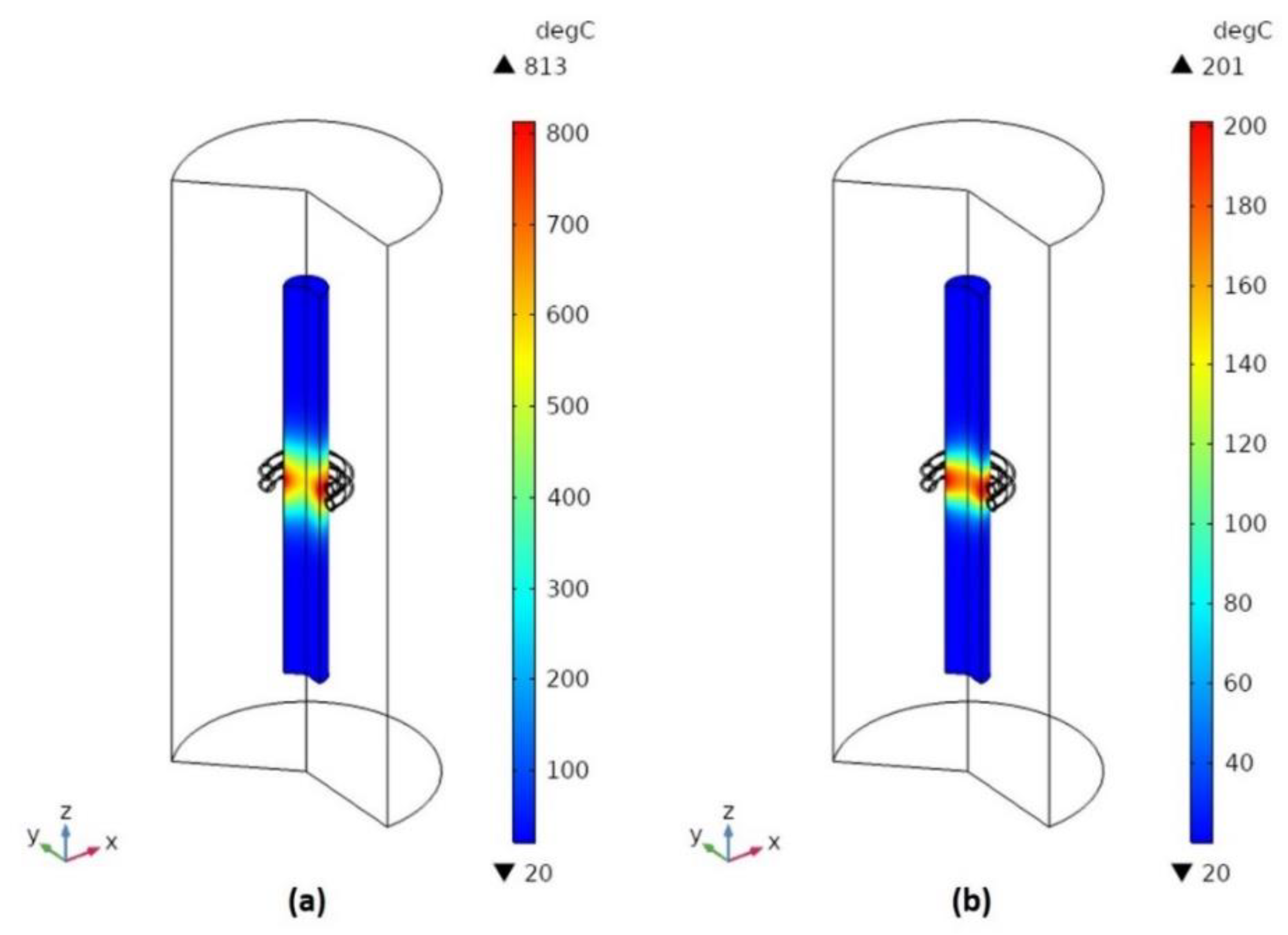
  • After converting the high-frequency induction heating system to the RLC circuit, the AC current (708 A) flowing through the induction heating coil was calculated and simulated. The temperature of the induction heating experiment of the AISI 1045 specimens was 797.9 °C and the simulated temperature was 813 °C.
  • To verify the hardening depth obtained by simulations, experiments were conducted, which produced the same 0.8 mm hardening depth.
  • As a result of comparing the experiment and simulation, it was confirmed that the accuracy of the simulation is high. Phase transformation simulations were more intuitive and efficient than previous simulations which predicted the curing area using only the existing heating and cooling temperatures [7,8]. It is expected that the high-frequency heat treatment and the heating coil shape can be further optimized through high-frequency heat treatment considering metal phase transformation simulations.

Author Contributions

Conceptualization, J.C. and S.L.; methodology, J.C.; software, J.C.; validation, J.C. and S.L.; formal analysis, J.C.; investigation, J.C.; resources, J.C.; data curation, J.C.; writing—original draft preparation, J.C.; writing—review and editing, J.C.; visualization, J.C.; supervision, S.L.; project administration, S.L.; funding acquisition, S.L. All authors have read and agreed to the published version of the manuscript.

Funding

This work was supported by the National Research Foundation of Korea (NRF) grant funded by the Korea government (MSIT) (No. 2020R1F1A1065983) and GNU Graduate Education and Researcher Program for Mechanical and Aerospace Engineers.

Conflicts of Interest

The authors declare no conflict of interest.

References

  1. Han, Y.; Yu, E.; Zhang, H.; Huang, D. Numerical analysis on the medium-frequency induction heat treatment of welded pipe. Appl. Therm. Eng. 2013, 51, 212–217. [Google Scholar] [CrossRef]
  2. Li, H.; He, L.; Gai, K.; Jiang, R.; Zhang, C.; Li, M. Numerical simulation and experimental investigation on the induction hardening of a ball screw. Mater. Des. 2015, 87, 863–876. [Google Scholar] [CrossRef]
  3. Lee, I.; Tak, S.; Pack, I.; Lee, S. Comparative Study on Numerical Analysis using Co-simulation and Experimental Results for High Frequency Induction Heating on SCM440 Round Bar. J. Soc. Aerosp. Syst. Eng. 2017, 11, 1–7. [Google Scholar] [CrossRef]
  4. Oh, D.-W.; Kim, T.H.; Do, K.H.; Park, J.M.; Lee, J. Design and Sensitivity Analysis of Design Factors for Induction Heating System. J. Korean Soc. Heat Treat. 2013, 26, 233–240. [Google Scholar] [CrossRef] [Green Version]
  5. Ji, H.; Wang, B.; Fu, X. Study on the induction heating of the workpiece before gear rolling process. In Proceeding of the 20th International ESAFORM Conference on Material Forming, Dublin, Ireland, 26–28 April 2017; Volume 1896, pp. 1–6. [Google Scholar] [CrossRef]
  6. Tak, S.-M.; Kang, H.-B.; Baek, I.-S.; Lee, S.-S. Improved workability using preheating in the electromagnetic forming process. J. Mech. Sci. Technol. 2019, 33, 2809–2815. [Google Scholar] [CrossRef]
  7. Choi, J.-K.; Park, K.-S.; Lee, S. Predicting the hardening depth of a sprocket by finite element analysis and its experimental validation for an induction hardening process. J. Mech. Sci. Technol. 2018, 32, 1235–1241. [Google Scholar] [CrossRef]
  8. Choi, J.-K.; Park, K.-S.; Lee, S. Prediction of High-Frequency Induction Hardening Depth of an AISI 1045 Specimen by Finite Element Analysis and Experiments. Int. J. Precis. Eng. Manuf. 2018, 19, 1821–1827. [Google Scholar] [CrossRef]
  9. Tong, D.; Gu, J.; Totten, G.E. Numerical simulation of induction hardening of a cylindrical part based on multi-physics coupling. Model. Simul. Mater. Sci. Eng. 2017, 25, 035009. [Google Scholar] [CrossRef]
  10. Rudnev, V.; Loveless, D.; Cook, R.; Black, M. Handbook of Induction Heating; Marcel Dekker: New York, NY, USA, 2003; p. 19. [Google Scholar]
  11. Korean Agency for Technology and Standards. KS D 0027, Methods of Measuring Case Depth for Steel Hardened by Flame or Induction Hardening Process; KATS: Maengdong-myeon, Korea, 2002.
  12. Alexander, C.; Sadiku, M.O. Fundamentals of Electric Circuits; McGraw-Hill: New York, NY, USA, 2012; pp. 613–673. [Google Scholar]
  13. Gao, K.; Qin, X.; Wang, Z.; Chen, H.; Zhu, S.; Liu, Y.; Song, Y. Numerical and experimental analysis of 3D spot induction hardening of AISI 1045 steel. J. Mater. Process. Technol. 2014, 214, 2425–2433. [Google Scholar] [CrossRef]
  14. Leblond, J.; Devaux, J. A new kinetic model for anisothermal metallurgical transformations in steels including effect of austenite grain size. Acta Metall. 1984, 32, 137–146. [Google Scholar] [CrossRef]
  15. Koistinen, D.; Marburger, R. A general equation prescribing the extent of the austenite-martensite transformation in pure iron-carbon alloys and plain carbon steels. Acta Metall. 1959, 7, 59–60. [Google Scholar] [CrossRef]
  16. Edelbauer, W.; Zhang, D.; Kopun, R.; Stauder, B. Numerical and experimental investigation of the spray quenching process with an Euler-Eulerian multi-fluid model. Appl. Therm. Eng. 2016, 100, 1259–1273. [Google Scholar] [CrossRef]
Figure 1. Measurement temperature setup for the AISI 1045 specimen during induction heating.
Metals 10 01484 g001
Figure 2. Measurement temperature results of AISI 1045 specimens during induction heating.
Metals 10 01484 g002
Figure 3. Configuration of high-frequency induction heating system.
Metals 10 01484 g003
Figure 4. Position of the measurement sections in resonance tank.
Metals 10 01484 g004
Figure 5. Voltage, frequency, and the representative resistance–inductance–capacitance (RLC) circuit of the resonance tank for measurement Section 1 and Section 2 and calculated current.
Metals 10 01484 g005
Figure 6. 3D model for induction hardening simulation.
Metals 10 01484 g006
Figure 7. Induction hardening simulation process. The dashed line does not couple during the simulation.
Metals 10 01484 g007
Figure 8. Thermal and electromagnetic properties with temperature of AISI 1045 steel. (a) Thermal conductivities, (b) specific heat, (c) relative permeability, (d) resistivity.
Metals 10 01484 g008
Figure 9. Induction heating simulation results: (a) 2 s after heating and (b) 4 s after cooling.
Metals 10 01484 g009
Figure 10. Phase change simulation results of AISI 1045 specimens: (a) austenite and (b) martensite.
Metals 10 01484 g010
Figure 11. The radial distribution of the phase composition.
Metals 10 01484 g011
Figure 12. Simulation results of martensite and a prediction of the hardening depth in the AISI 1045 specimen.
Metals 10 01484 g012
Figure 13. Comparison of hardening depth results: from experiments and simulations.
Metals 10 01484 g013
Figure 14. Optical microscopic images of the AISI 1045 specimen and its hardening depth.
Metals 10 01484 g014
Table 1. Measurement hardening depth results of the AISI 1045 specimen.
Depth (mm)Vickers Hardness (Hv)Rockwell Hardness (HrC)
0.0552050.5
0.1057353.8
0.1558054.2
0.2060055.3
0.3058454.4
0.4059054.7
0.5048548.1
0.6049849
0.7049248.6
0.8050049.1
0.9043143.8
1.0040941.8
Table 2. Measurement results for the alternating current voltage and frequency in measurement Section 1 and Section 2.
AC Voltage (V)Frequency (kHz)
Measurement Section 1130 ± 5.3%241.7 ± 0.8%
Measurement Section 2194 ± 6.7%242 ± 0.6%
Table 3. Ferrite to austenite, temperature-dependent functions.
Temperature (°C)K (l/s)L (l/s)
7500.221
7700.531
7901.050.97
8102.020.94
8304.550.87
8405.60.76
8607.370.45
88010.770
900200
Table 4. Austenite to bainite, temperature-dependent functions.
Temperature (°C)F (l/s)G (l/s)
3400
3500.014
4500.0670
55000.067
Table 5. Austenite to bainite, temperature-rate-dependent functions.
Temperature Rate (K/h)H (l)
−43,0000.2
−15,0001
−72001.5
−15000.22
−7000.1
−700.0044
Table 6. Austenite to martensite parameters.
ParameterValue
MS370 (°C)
β0.011 (1/K)
Publisher’s Note: MDPI stays neutral with regard to jurisdictional claims in published maps and institutional affiliations.

