Prediction of Fatigue Crack Growth Behaviour in Ultrafine Grained Al 2014 Alloy Using Machine Learning

Abstract

The present work investigates the relationship between fatigue crack growth rate (da/dN) and stress intensity factor range (∆K) using machine learning models with the experimental fatigue crack growth rate (FCGR) data of cryo-rolled Al 2014 alloy. Various machine learning techniques developed recently provide a flexible and adaptable approach to explain the complex mathematical relations especially, non-linear functions. In the present work, three machine algorithms such as extreme learning machine (ELM), back propagation neural networks (BPNN) and curve fitting model are implemented to analyse FCGR of Al alloys. After tuning of networks with varying hidden layers and number of neurons, the trained models found to fit well to the tested data. The three tested models are compared with each other over the training as well as testing phase. The mean square error for predicting the FCG of cryo-rolled Al 2014 alloy by BPNN, ELM and curve fitting methods are 1.89, 1.84 and 0.09 respectively. While the ELM models outperform the rest of models in terms of training time, curve fitting model showed best performance in terms of accuracy over testing data with least mean square error (MSE). In terms of local optimisation, back propagation neural networks excel the other two models.

1. Introduction

Failure of metals by fatigue was common even in the pre-historical, Bronze and Iron ages. However, fatigue failures were identified and analysed extensively during the middle of the nineteenth century when Wohler fatigue tested full-sized railway axles, in Germany [1]. In initial stages of fatigue analysis, the components were designed for safe-life approach known as stress-based approach. The materials were tested under cyclic stress amplitude until failure occurs to estimate the infinite life of the material. Second, fail-safe criteria, also known as strain-based approach, were used. In this case, the materials were tested to find out the strain amplitude at which the material fails by testing at stress values close to the tensile strength which enables to design the system for fail-safe. Both these methods have the drawback of wastage of materials like discarding the healthy material in case of safe-life method and redundancy in case of fail-safe method. Hence, the third method, damage tolerance approach was introduced, with the advent of fracture mechanics, to identify the potential crack and repair it, before it becomes critical. The mechanisms of crack origin, growth of small cracks into a long crack, crack arrest and growth and final failure mechanisms due to several influencing factors such as material property, environment, nature of loading, cyclic stress amplitude and cyclic stress intensities were reported by Stanzl-Tschegg [2]. The theory of linear elastic fracture mechanics (LEFM) determined by stress analysis, and expressed as a function of stress and crack size has been developed using a stress intensity factor (K). LEFM is used for material conditions which are predominantly linear elastic during the fatigue process and explores basic theory of fracture. As long as the condition of small scale yielding is met, LEFM is applicable, else elastic-plastic method is adopted.

The important parameter that is used in fracture mechanics to predict the crack growth is stress intensity factor. The rate at which the crack grows (da/dN) during the cyclic loading depends on the stress intensity factor range (∆K) which in turn depends on the growing crack size (a). Thus, a fatigue crack growth (FCG) experiment containing a plot of da/dN versus ∆K, contains three regions, namely, threshold region or crack initiation region, stable crack growth region and unstable crack growth region. In the crack initiation region, the crack growth rate could be in the order of around 10⁻⁸ mm/cycle; in the stable crack growth region, the crack growth rate could be in the order of 10⁻⁶ to 10⁻⁴ mm/cycle; and in the unstable crack growth regime, the crack growth rate is greater than 10⁻³ mm/cycle. The three most important relationships used to characterise the fatigue crack growth problems are Paris equation, Walker equation and NASGRO equation. Paris equation defines the stable crack growth region of FCG plot that does not account for the stress ratio; whereas Walker equation does account for stress ratio yet only for the stable crack growth region. NASGRO equation, that was developed jointly by Southwest research Institute and NASA, accounts for all the three regions (crack initiation, stable and unstable crack growth regions), stress ratio effect as well as crack-closure effects.

Nowadays, in the era of Industry 4.0, data can be shared and retrieved from anywhere around the globe using cloud-based data storage methods. Hence, the shortcomings in the existing failure predictions methods, such as inconsistency in the prediction and not able to solve complex non-linear damage mechanics [3] can be overcome by the advent of advanced data collection and interpretation methods such as support vector mechanisms, decision trees and random forests approaches [4]. The data science in combination with advanced algorithms developed using programming languages such as Python can be used to train a machine in order to perform certain function with minimal error is generally termed as machine learning (ML). Data driven constitutive modelling was studied by Versino et al. [5] for plastic deformation of metallic materials. Dimiduk et al. [6] reviewed the importance and impact of ML and artificial intelligence (AI) on the materials, process and structural engineering and emphasised that data-driven approaches are the future in solving long standing technological challenges like fatigue life prediction. Haynes e al. [7] reported that the NASGRO and AFGRO approaches to predict the fatigue life cycles were found to be incorrect by ten-folds because of its inability to predict equivalent initial flaw size. An et al. [8] used Bayesian approach using Markov Chain Monte Carlo (MCMC) technique to predict fatigue life of the turbine components using available field data. Using Bayesian approach was reported advantageous over regression method as it effectively utilises the prior data and its ability to choose appropriate statistical model. Doh and Lee [9] observed from their result in predicting the fatigue life of HS40R steel that the Bayesian approach using MCMC technique was useful in enumerating the uncertainty of the unknown parameters. Rovinelli et al. [10] used Bayesian approach to identify the driving force for small fatigue cracks using multimodal data sets using 4D experiments in situ with small propagating cracks and crystal plasticity simulations. Bayesian models work with predictive distributions but not with the initial distributions whose weights arise from the posterior distribution and helps to find out the initial distributions [11]. Ali [12] used deep learning approach to reduce the time and cost while predicting fatigue life of stiffened sections using Monte-Carlo simulation. Pujol et al. [13] used feed forward neural network with cumulative distribution of failed steel components and step-stress method which yielded a better fit when compared to the standard lognormal distribution method. Schwarzer et al. [14] used ML approach that consists of an architecture of neural networks containing several components, such as feed forward neural networks, graphical convolution networks and recurrent neural network. The predicted values were in good agreement with the experimental results and the significant benefit of ML approach is its speed. Pierson et al. [15] used convolution neural network approach to predict microstructural sensitive crack growth in Al-Mg-Si alloy as predicting such microstructurally small cracks using Paris-Erdogan law exhibit greater deviation in their growth behaviour. Such deviation in predicting the fatigue life using Paris-Erdogan law was observed from the fatigue life study of additively manufactured ASi10Mg alloy [16].

Nguyen et al. [17] forecasted the crack propagation problem using two deep learning models namely, multi-layer neural network and long-short term memory method. It was concluded that multilayer neural network is less effective but cheaper than long-short term memory method. Wang et al. [18] estimated the fatigue stress concentration factor using ELM which predicts the stress concentration factor favourably against the existing empirical relationships. The relevance vector mechanism (RVM) was used to predict the useful remnant life of a structure by Zio et al. [19]. Genetic algorithms to predict the fatigue life of heat-treated Al 2024 alloy was employed by Mohanty et al. [20] but comparisons with other ML algorithms are not made. Wang et al. [21] compared three ML-based algorithms, namely, extreme learning machine (ELM), radial basis function network (RBFN) and genetic algorithms optimised back propagation network (GABP) to predict FCG calculations of Al2024-T351 alloy. The ELM method was found to be the best among the three as it led to better global optimisation and extrapolation ability. Radial basis function network method was used by Zhang et al. [22] to predict the fatigue crack growth. However, no attempts were made to study the significant difference in using particular ML algorithm and its influence on the predictive capability.

In this work, the FCG of cryo-rolled Al 2014 alloy predicted using ELM and back propagation neural network (BPNN) is compared with the general curve fitting technique. The BPNN is a type of multi-layer neural network method. Neural networks are methods that power deep learning that contain machine called perceptron. The perceptron in neural networks are equivalent to biological neurons in order to impart the ability of sensing and remembering like a human being. To solve linear problems, single layer of perceptron with a step function is enough but to solve non-linear problems, the neuron network required two or more hidden layers and it is known as multi-layer neuron network. For a set of input parameters, a weight set and bias parameters are assigned to hidden neuron nodes which gives an output. In order to calculate the hidden layer function, the output values are fed into one of the activation functions like sigmoid, tanh, rectified linear unit (ReLU) and softplus functions. The activation function decides which node to be fired and make non-linearity feasible. Loss function or cost function is minimised during the training process to evaluate and ensure the correct performance of the model. In BPNN, the gradient of the loss function is calculated by back propagation with respect to the weights of network and uses this gradient to update the hyper parameters. The back-propagation computes gradient by applying chain rule computing gradient one layer at a time starting from last layer and propagate towards input. On the other hand, ELM is a single layer feed forward network (SLFN) without the need to tune the hidden layer [23]. ELMs can outperform support vector machines in both quantitative and qualitative data analysis. The support vector machines require to solve quadratic problems [24] whereas in the ELM method, instead of tuning the hidden layer, it arbitrarily choose a hidden node and only need to calculate weight that links the output and the hidden node, analytically [25,26]. Hence, it would be interesting to compare deep learning algorithms based on multi-layer back propagation and a single layer feed forward to predict the FCG of the cryo-rolled Al alloy in the present work. The experimental fatigue crack growth data of this alloy reported in our earlier work [27] were taken to train the various ML models in this work in order to explore its predictive capabilities of fatigue failure of metallic materials.

2. Materials and Methods

2.1. Experimental Method

For the present investigation, Al 2014 alloy was used. The fatigue crack growth rate (FCGR) tests were performed on the cryo-rolled CR and the samples annealed after cryo-rolling following ASTM 647-08 standard using the compact tension (CT) specimen. The samples are annealed after cryo-rolling at 100 °C, 150 °C, 200 °C and 250 °C which are termed as CR100, CR150, CR200 and CR250 respectively. The FCGR test usually involves the notched specimen that is subjected to cyclic loading and acceptably pre-cracked under fatigue. The FCGR (da/dN) is expressed as a function of stress intensity factor range (ΔK) and is defined as material resistance to the stable crack extension under fatigue loading. The stress ratio R ratio for all processed condition during FCGR tests in this work was maintained at 0.1. The experimental method and data are part of our work on the study of the structure–property relationship of ultra-fine grained Al 2014 alloy processed using cry-rolling [26].

2.2. Machine Learning Methods

2.2.1. Data Pre-Processing

Normalisation is a technique often applied as part of data preparation for machine learning. Normalisation of data helps in improving the performance of the model. The goal of normalisation is to change the values of numeric columns in the dataset to a common scale, without distorting differences in the ranges of values. For machine learning, every dataset does not require normalisation. It is required only when features have different ranges. The mean of entire dataset is calculated and subtracted from each sample and the output is divided by the standard deviation of the dataset. Normalised data are used as input for the machine learning algorithms.

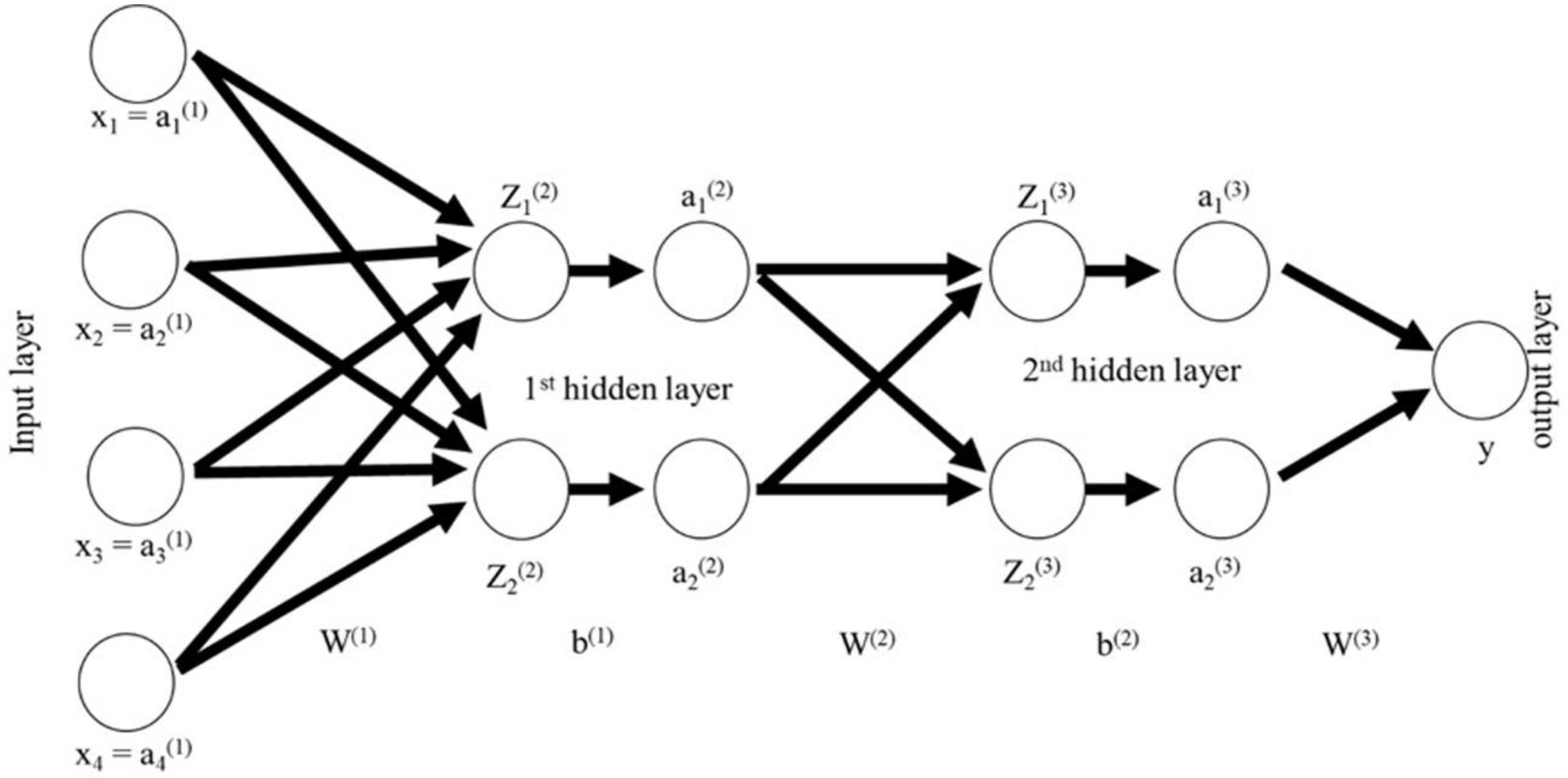
2.2.2. Back Propagation Neural Network

Because of its learning ability and flexible structure, back propagation algorithm has been one of the most widely used machine learning algorithms. Gradient of the loss function is calculated by back propagation with respect to the weights of network and the algorithm uses this gradient to update the hyper parameters. The back-propagation computes gradient by applying chain rule computing gradient one layer at a time starting from last layer and propagate towards input as shown in the Figure 1.

Each unit in neural network is called neuron and neurons are arranged along layers. Each network contains input layer, hidden layer and output layer. The current backpropagation model is built in Tensorflow with Keras backend. The model contains an architecture as shown in the Figure 1 with two hidden layers, an input and an output layer. The input layer and output layer and three hidden layers. Let the dataset X = $\left\{x_1,x_2,x_3,\dots x_n\right\}$, Wⁱ = {$w_1^i{w}_2^i,w_3^i\dots .,w_n^i$} and bⁱ = {$b_1^i{b}_2^i,b_3^i\dots .,b_n^i$} be the weight set and bias parameter to the ith hidden node respectively. Then, the result (Z) is given by Equation (1):

$$Z^i={\displaystyle \sum }_{j=1}^n{w}_j^i{x}_j+b_j^i$$

(1)

In order to calculate the hidden layer values, the value of Z has to be fed into the activation function. The activation function is accountable to transform the summed weighted input to activate the output of the node. The significance of activation function in neural network is to make the network non-linear and to execute the correct node. The activation function used in the model is ReLU as it works better for the fatigue data compared to sigmoid and tanh activation functions. ReLU will give the input directly as output if the input is positive else it will return zero. It is mathematically expressed in Equation (2) as,

$$x=\{\begin{array}{c}0:x<0\\ x:x\ge 0\end{array}$$

(2)

As BPNN has more than one hidden layer, it leads to vanishing gradient problem if any activation function other than ReLU is used. After calculating the hidden layers, we may get n values of hidden nodes which can be expressed as h = {h₁, h_2, h_3,…h_n}, then the corresponding weight set, W^h = {$w_1^h,w_2^h,w_3^h\dots .,w_n^h$} and bias set, b^h = {$b_1^h,b_2^h,b_3^h\dots .,b_n^h$}. Also, the result of the nodes Z is given by Equation (3),

$$Z={\displaystyle \sum }_{j=1}^n{w}_j^h{x}_j+b_j^h$$

(3)

Finally, the output ($\overline{Y}$) can be calculated as the function of Z as $\overline{Y}=f\left(Z\right)$. To evaluate the network during training phase, a loss function or cost function is used, which has to be minimised for the network to navigate correctly. The loss function used to optimise the weights of the model is mean square error (MSE) function which is given by the following Equation (4).

$$E=\frac{1}{k}{\displaystyle \sum }_{j=1}^k{\left(\overline{Y}-Y\right)}^2$$

(4)

In the Equation (4), E is the error, $\overline{Y}$ is the calculated value and Y is the expected value for k number of data in the data set. The optimiser used to minimise the loss function is ‘adam’.

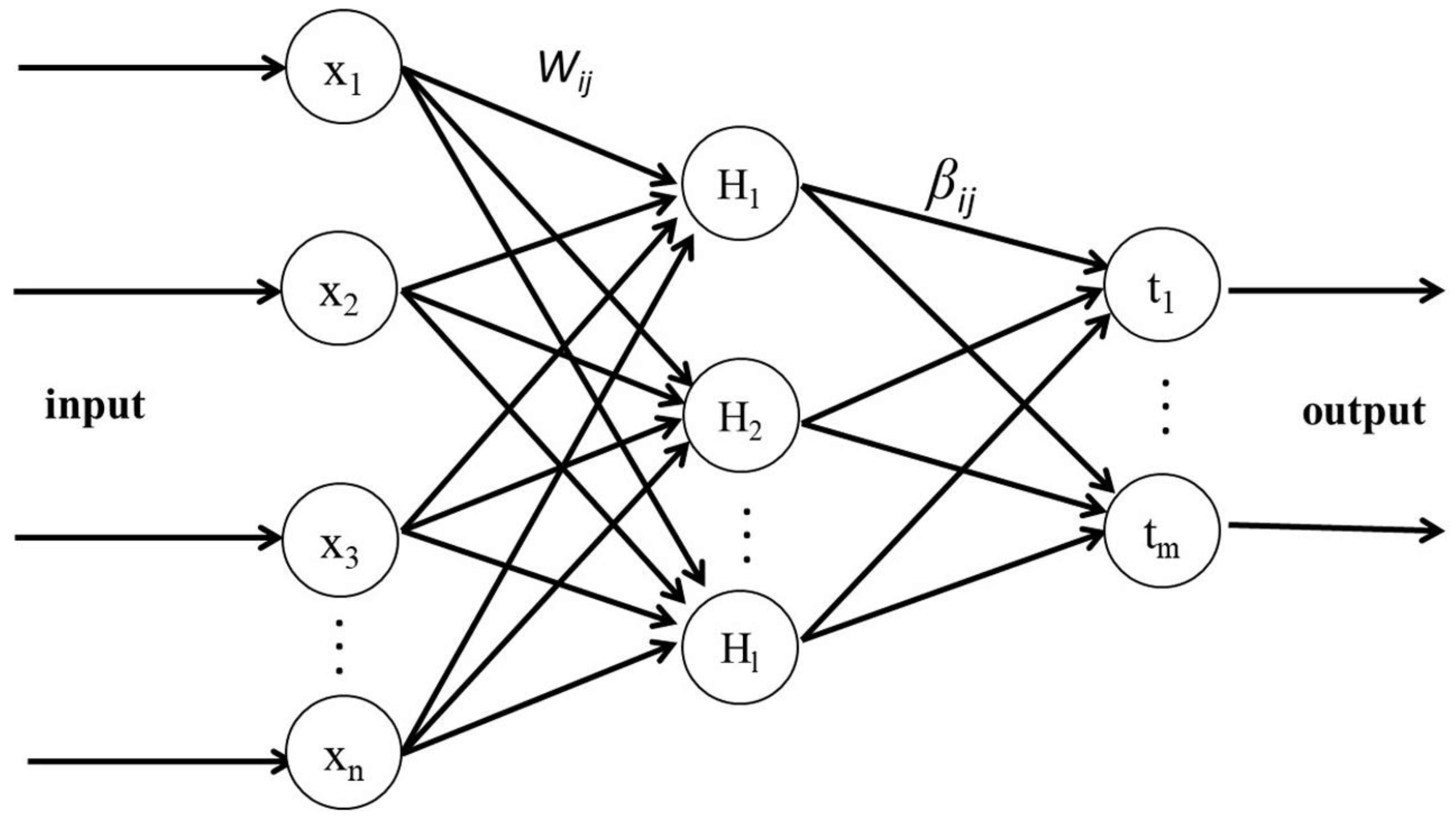
2.2.3. Extreme Learning Machine

Extreme learning machine contains only one hidden layer, in other words, it is similar to three-layer feed forward neural network with single hidden layer architecture as shown in the Figure 2.

In contrast to BPNN, the nodes of the ELM model need not be tuned or adjusted. Instead, the weight and bias parameters of the activation functions are randomly generated by the continuous probability distribution [18]. Hence, the activation function of ELM should satisfy a condition that it should be an infinitely differentiable function. The infinitely differentiable activation functions available are sigmoid, tanh, RBL functions.

$$f\left(x\right)=\frac{1}{1+x}$$

(5)

$$f\left(x\right)=\frac{e^x-e^{-x}}{e^x+e^{-x}}$$

(6)

The Equation (5) is the sigmoidal function and the Equation (6) is the tanh function, respectively which are used with ELM model and then optimised using the loss function MSE. For the current model, ‘high performance ELM toolbox’ was used which is based on python. Model is experimented with both sigmoid and tanh activation functions and plotted.

3. Results and Discussion

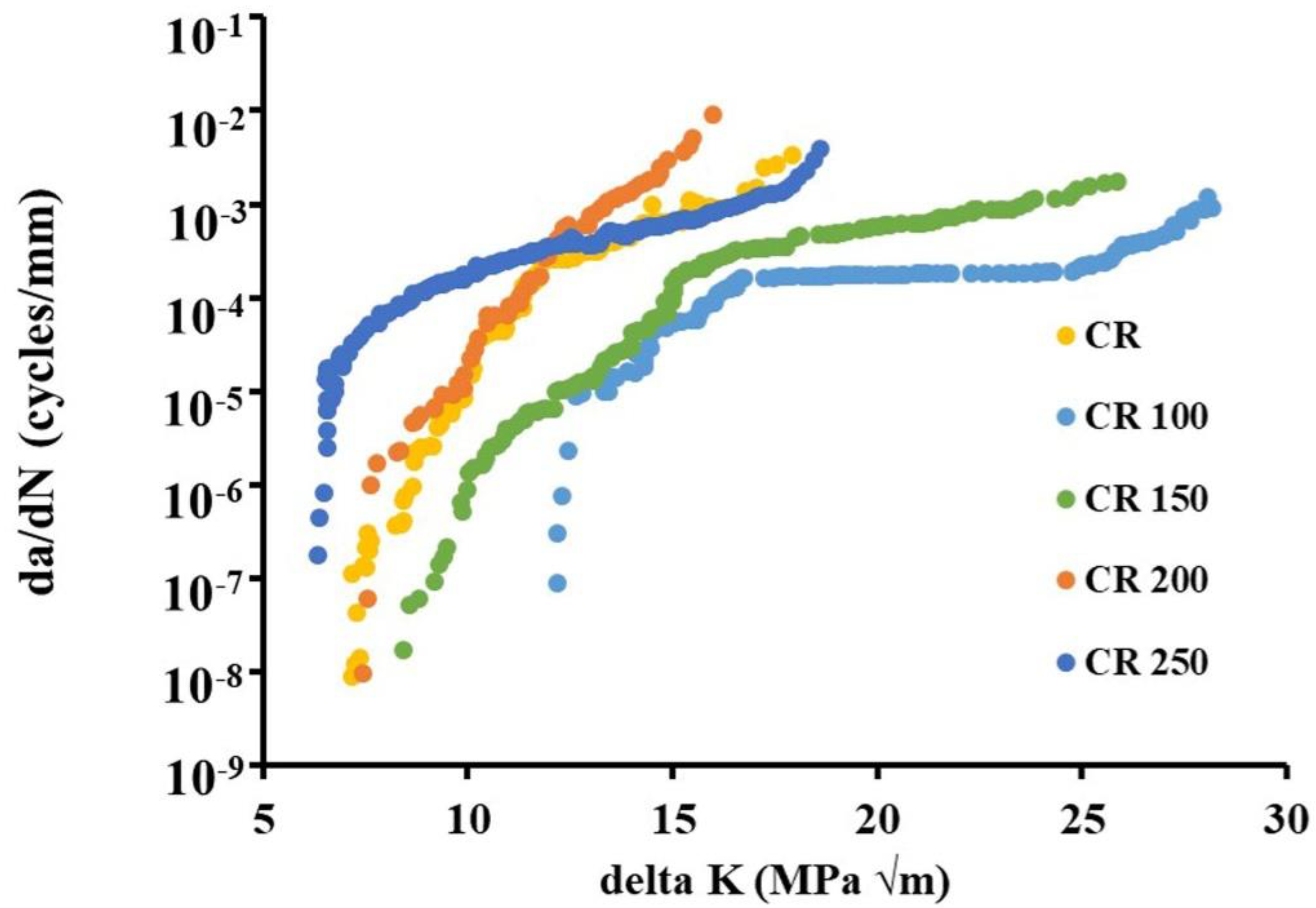
3.1. Experimental Data

Fatigue crack growth tests were conducted on the simply cryo-rolled sample and on cryo-rolled samples after being annealed at four temperatures in the range 100–250 °C to estimate its crack growth resistance in this work. Usually, fatigue crack growth test results cover the range of ΔK (stress intensity factor range) and fatigue crack growth rate (FCGR). In these experiments, fatigue crack growth rate (da/dN) is plotted with respect to ΔK (stress intensity factor range) on log-log plot. Some part of the experimental data on structure–property relationship of ultra-fine grained Al 2014 alloy obtained by cryo-rolling [27] were used to train and test the ML algorithms in this work. The experimental data are presented in the Figure 3.

The experimental data correspond to the simply cryo-rolled (CR) sample and the cryo-rolled samples after annealing. As the CR 250 sample exhibited smooth Paris law regime, the data of these samples were used to train the algorithms; while the data of the other samples CR, CR100, CR150 and CR200 are used to test the trained algorithms. In the present investigation, the fatigue crack growth test results for cryo-rolled and annealed samples after cryo-rolling showed two important findings: (i) Fatigue crack growth resistance of bulk UFG Al 2014 alloy developed by CR exhibited lower fatigue crack growth resistance and higher crack initiation stress intensity factor ΔKth as compared to the ST alloy; (ii) on annealing, the fatigue crack growth resistance and crack initiation stress intensity factor ΔKth improved compared to the CR alloy. The maximum resistance to crack growth was imparted by CR100 sample which was annealed at 100 °C after cryo-rolling.

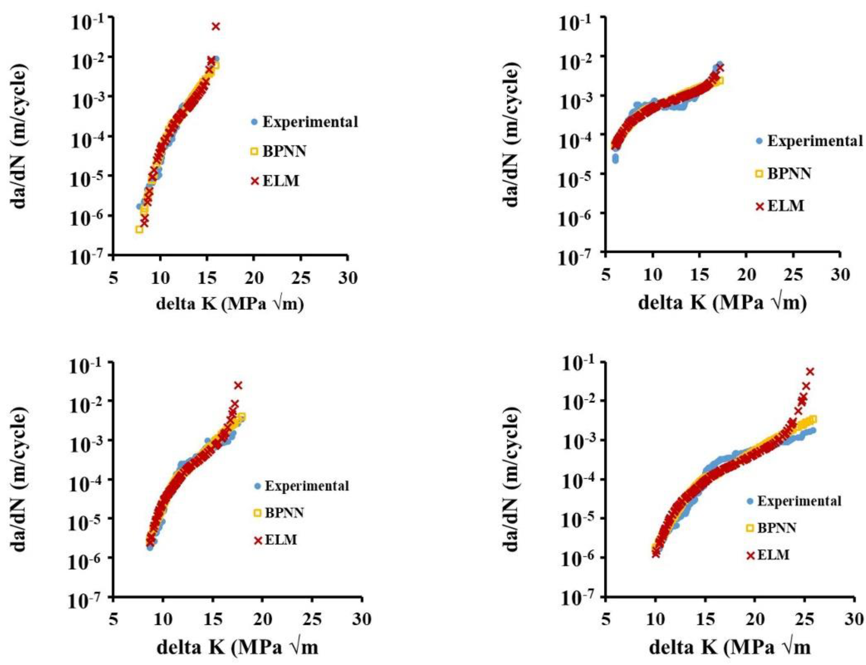
3.2. Machine Learning

We tried to predict the material constants by using ML algorithms. Considering the complexity involved in modelling the relationship between crack growth rate (da/dN) and stress intensity factor range (∆K) which are not linear even in the Paris region as well as diverse effects of stress ratio on different materials, most existing models cannot capture these non-linearities. However, most recently, to fit any type of data with being flexibility and adaptability as its strengths, machine learning algorithms handle the non-linear relationships elegantly. In fact, algorithms like principal component analysis can capture the hidden factors responsible for certain phenomenon. Thus, machine learning method provides an alternative and flexible approach for modelling of fatigue crack growth rate because of their non-linear approximation and multivariable learning ability which makes it advanced and promising. The tests to evaluate the trained models were implemented over different dataset.

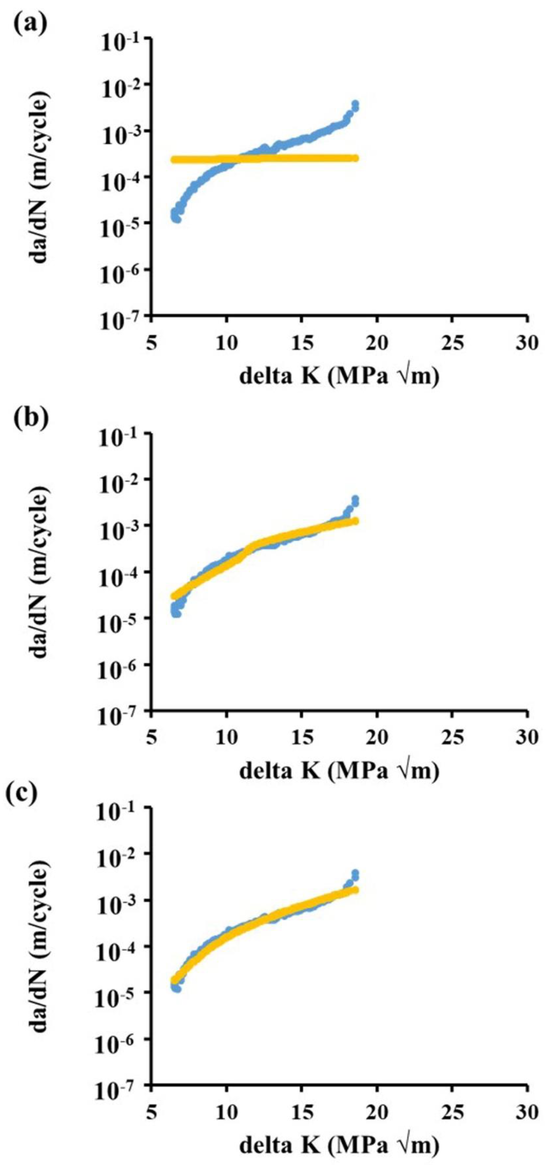
Back Propagation Neural Networks

Overfitting is a modelling error that occurs when a function is too closely fit to a limited set of data points. It occurs when a model learns the detail and noise in the training data in such a way that it predicts the particular set of data exactly but fails to predict a new set of data. This means, overfitting is defined by low bias in the parameters but with high sampling variance. Overfitting is an issue, as there are very few theories available to guide the analysis.

The best of the training models was selected (CR250) after implementing trial and error over number of neurons as well as number of epochs. The influence of epochs on BPNN model are presented in the Figure 4. In Figure 4a, only one epoch was used and hence the prediction of the data deviated drastically from the experimental plot. There is a considerable deviation from the experimental curve to the predicted curves in Figure 4a,b, where 1 and 5 epochs respectively, were used. However, after implementing 10 epochs (Figure 4c), the simulated curve almost matched with the experimental curve.

The number of hidden neurons affect the accuracy of the ELM model which are determined based on trial and error method. The prominent factor in determining the accuracy of model in ELM is the number of neurons in hidden layer. Extreme learning machine (ELM) is an emerging MLA, which is a single-hidden layer feed-forward neural network (SLFN). The structure of ELM is similar with the three-layer FFNN. In the ELM, the layers are fully connected. Additionally, an infinitely differentiable function must be selected as the activation function of the hidden layer, which is usually a sigmoid function. The effect of number of neurons on ELM model using sigmoid function and tan h function is shown in Figure 5. The sigmoid function completely missed the experimental plot with single neuron (Figure 5a); it somewhat tried to match the experimental plot in Figure 5b when 5 neurons were used, and completely in line with the experimental plot when 10 neurons were used (Figure 5c). Similarly, while using tan h function also, the prediction capability increases with increasing the number of neurons from 1 (Figure 5d) to 5 (Figure 5e) and then to 13 (Figure 5f).

The tested data using BPNN and ELM models along with experimental data trends for all the tested materials are shown in the Figure 6. It can be clearly observed from the Figure 6a that the simply cryo-rolled (CR) materials exhibited maximum slope value and the CR100 annealed material in Figure 6b exhibited least slope. Meanwhile, the other heat treated cryo-rolled materials (Figure 6c,d) had exhibited FCG behaviour intermittent to CR and CR100 samples. The ML simulated curves are almost in agreement with the experimental data. The BPNN model approximates the local data points accurately whereas the ELM model extrapolate the critical region, i.e., unstable crack growth region precisely. BPNN was unable to explain the upper tail region of the curve, while the ELM model explained the upper tail of the curve elegantly.

Total of 135 data points were investigated for the test case. The MSE value for the BPNN model stands at 1.89. The MSE value for ML algorithms used and polynomial curve fitting are presented in

Table 1. Mean square error (MSE) of machine learning (ML) algorithms compared with polynomial curve fit method.

Model Name	MSE
BPNN	1.89
ELM	1.84
Curve fitting	0.09

. The ELM-based prediction is plotted below similar to BPNN, and 135 samples were investigated for the test case. The MSE value for the ELM model stands at 1.84. The same is observed in the estimated test cases. Because of its greater ability to interpret the data at the critical stress regions, ELM is ranked well than the rest of the two models. The curve fitting model-based prediction is plotted in Figure 7 and 135 samples are investigated for this case as well. The MSE for curve fitting model is the best of the three with 0.09. The assumed 5th degree function modelled well for the data even though any form of function is determined based on trial and error. Figure 6 also explains the ability of ELM model for its efficiency in data extrapolation compared to the rest of models.

The influence of cryo-rolling on fatigue limit is attributed to the presence of ultrafine grains which increases the crack initiation phase by reducing the stress concentration near the crack tip and thereby increasing the fatigue strength of cryo-rolled (CR) alloy. On the other hand, influence of cryo-rolling followed by annealing is attributed to the combined recovery and recrystallisation process, which enhances the plastic zone size near the crack tip due to crack tip/precipitate interaction resulting in enhanced fatigue crack growth resistance at low temperature annealing [28]. The similar fatigue behaviour in other Al alloys were also reported in the literature [16,29,30]. These differences in the Paris law regime were clearly interpreted by ML algorithms. The crack initiation regime and unstable crack growth regime were extrapolated as insufficient data recorded in these regions. All the three models fit well to the test data and have proven their credibility and ease compared to numerical-based simulation for substantiating fatigue life of Al alloys. However, the most important aspect of crack growth rate estimation is to predict the failure. ELM has been found to be elegant in this aspect by fitting well to the data at the critical stress region.

4. Conclusions

In this work, the fatigue crack growth calculation based on MLA is proposed and the relationship between fatigue crack growth rate and stress intensity factor has been investigated using three MLAs. The trained models are validated by using testing data of different dataset. The results indicate that the MLAs can fit the nonlinearities of fatigue crack growth rate very well, and the MLA-based fatigue crack growth shows fairly good performance for different experimental data. Comparison of the three models is summarised below:

• Machine learning techniques are way too easy and flexible as compared to designing numerical equations because of their non-linear activation functions.
• In back propagation, accuracy increases till certain number of epochs and starts decreasing after that, hence optimum number of epochs is determined by experimentation.
• In ELM model, optimum number of neurons in hidden layer affects the accuracy and is found by experimenting.
• Activation functions in both the above neural networks play a critical role as they are prominent in explaining non-linearity.
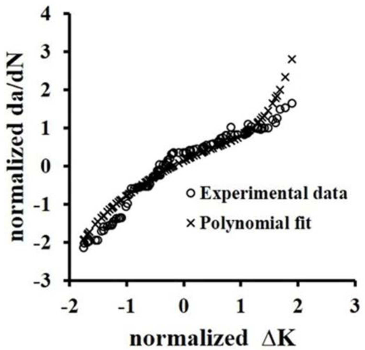
• Curve fitting model requires initial assumption about the type of function to be used and also fails if model fits other than polynomial functions as they are difficult to assume, for example log function. ELM is the best model followed by back propagation neural networks because of its ability to model non-linearity.
• The non-linearity, even in the Paris region of fatigue crack growth of the materials can be better predicted using ML algorithms rather than using Paris law or polynomial curve fitting techniques.
• The ELM model, the quickest of the two ML models used, predicts the unstable crack growth region more accurately when compared to BPNN and polynomial curve fitting techniques.

References

1. Kardomateas, G.A.; Geubelle, P.H. Fatigue and Fracture Mechanics in Aerospace Structures. In Encyclopedia of Aerospace Engineering; Blockley, R., Shyy, W., Eds.; Wiley: Chichester, UK, 2010. [Google Scholar]
2. Stanzl-Tschegg, S.E. When do small fatigue cracks propagate and when are they arrested? Corros. Rev. 2019, 37, 397–418. [Google Scholar] [CrossRef]
3. Schütz, W. Fatigue life prediction of aircraft structures—Past, present and future. Eng. Fract. Mech. 1974, 6, 745–762. [Google Scholar] [CrossRef]
4. Bock, F.E.; Aydin, R.C.; Cyron, C.J.; Huber, N.; Kalidindi, S.R.; Klusemann, B. A Review of the Application of Machine Learning and Data Mining Approaches in Continuum Materials Mechanics. Front. Mater. 2019, 6, 1–23. [Google Scholar] [CrossRef] [Green Version]
5. Versino, D.; Tonda, A.; Bronkhorst, C.A. Data driven modeling of plastic deformation. Comput. Methods Appl. Mech. Eng. 2017, 318, 981–1004. [Google Scholar] [CrossRef] [Green Version]
6. Dimiduk, D.M.; Holm, E.; Niezgoda, S.R. Perspectives on the Impact of Machine Learning, Deep Learning, and Artificial Intelligence on Materials, Processes, and Structures Engineering. Integr. Mater. Manuf. Innov. 2018, 7, 157–172. [Google Scholar] [CrossRef] [Green Version]
7. Haynes, R.; Joshi, G.; Bradley, N. Machine learning-based prognostics of fatigue crack growth in notch pre-cracked aluminum 7075-T6 rivet hole. Proc. Annu. Conf. PHM Soc. 2018, 10, 1–8. [Google Scholar]
8. An, D.; Choi, J.-H.; Kim, N.H.; Pattabhiraman, S. Fatigue life prediction based on Bayesian approach to incorporate field data into probability model. Struct. Eng. Mech. 2011, 37, 427–442. [Google Scholar] [CrossRef] [Green Version]
9. Doh, J.; Lee, J. Bayesian estimation of the lethargy coefficient for probabilistic fatigue life model. J. Comput. Des. Eng. 2017, 5, 191–197. [Google Scholar] [CrossRef]
10. Rovinelli, A.; Sangid, M.D.; Proudhon, H.; Ludwig, W. Using machine learning and a data-driven approach to identify the small fatigue crack driving force in polycrystalline materials. NPJ Comput. Mater. 2018, 4, 35. [Google Scholar] [CrossRef] [Green Version]
11. Castillo, E.F.; Muñiz-Calvente, M.; Canteli, A.F.; Blasón, S. Fatigue Assessment Strategy Using Bayesian Techniques. Materials 2019, 12, 3239. [Google Scholar] [CrossRef] [Green Version]
12. Ali, H. Accelerated Fatigue Reliability Analysis of Stiffened Sections Using Deep Learning. Master’s Thesis, National University of Sciences and Technology, Islamabad, Pakistan, 2018; pp. 1–53. Available online: https://hdl.handle.net/11244/320947 (accessed on 16 July 2020).
13. Pujol, J.C.F.; Pinto, J.M.A. A neural network approach to fatigue life prediction. Int. J. Fatigue 2011, 33, 313–322. [Google Scholar] [CrossRef]
14. Schwarzer, M.; Rogan, B.; Ruan, Y.; Song, Z.; Lee, D.Y.; Percus, A.; Chau, V.T.; Moore, B.A.; Rougier, E.; Viswanathan, H.S.; et al. Learning to fail: Predicting fracture evolution in brittle material models using recurrent graph convolutional neural networks. Comput. Mater. Sci. 2019, 162, 322–332. [Google Scholar] [CrossRef] [Green Version]
15. Pierson, K.; Rahman, A.; Spear, A.D. Predicting Microstructure-Sensitive Fatigue-Crack Path in 3D Using a Machine Learning Framework. JOM 2019, 71, 2680–2694. [Google Scholar] [CrossRef] [Green Version]
16. Ch, S.R.; Raja, A.; Jayaganthan, R.; Vasa, N.; Raghunandan, M. Study on the fatigue behaviour of selective laser melted AlSi10Mg alloy. Mater. Sci. Eng. A 2020, 781, 139180. [Google Scholar] [CrossRef]
17. Nguyen, D.L.H.; Do, D.T.T.; Lee, J.; Rabczuk, T.; Nguyen-Xuan, H. Forecasting Damage Mechanics by Deep Learning. Comput. Mater. Contin. 2019, 61, 951–977. [Google Scholar] [CrossRef]
18. Wang, B.; Zhao, W.; Du, Y.; Zhang, G.; Yang, Y. Prediction of fatigue stress concentration factor using extreme learning machine. Comput. Mater. Sci. 2016, 125, 136–145. [Google Scholar] [CrossRef]
19. Zio, E.; Di Maio, F. Fatigue crack growth estimation by relevance vector machine. Expert Syst. Appl. 2012, 39, 10681–10692. [Google Scholar] [CrossRef]
20. Mohanty, J.; Mahanta, T.; Mohanty, A.; Thatoi, D. Prediction of constant amplitude fatigue crack growth life of 2024 T3 Al alloy with R-ratio effect by GP. Appl. Soft Comput. 2015, 26, 428–434. [Google Scholar] [CrossRef]
21. Wang, H.; Zhang, W.; Sun, F.; Zhang, W. A Comparison Study of Machine Learning Based Algorithms for Fatigue Crack Growth Calculation. Materials 2017, 10, 543. [Google Scholar] [CrossRef] [Green Version]
22. Zhang, W.; Bao, Z.; Jiang, S.; He, J. An Artificial Neural Network-Based Algorithm for Evaluation of Fatigue Crack Propagation Considering Nonlinear Damage Accumulation. Materials 2016, 9, 483. [Google Scholar] [CrossRef] [Green Version]
23. Huang, G.-B.; Zhou, H.; Ding, X.; Zhang, R. Extreme Learning Machine for Regression and Multiclass Classification. IEEE Trans. Syst. Man Cybern. Part B Cybern. 2011, 42, 513–529. [Google Scholar] [CrossRef] [PubMed] [Green Version]
24. Huang, G.-B. An Insight into Extreme Learning Machines: Random Neurons, Random Features and Kernels. Cogn. Comput. 2014, 6, 376–390. [Google Scholar] [CrossRef]
25. Huang, G.-B.; Chen, L.; Siew, C.-K. Universal Approximation Using Incremental Constructive Feedforward Networks With Random Hidden Nodes. IEEE Trans. Neural Netw. 2006, 17, 879–892. [Google Scholar] [CrossRef] [PubMed] [Green Version]
26. Huang, G.-B.; Chen, L. Convex incremental extreme learning machine. Neurocomputing 2007, 70, 3056–3062. [Google Scholar] [CrossRef]
27. Joshi, A.; Yogesha, K.K.; Raja, A.; Owalabi, G.; Jayaganthan, R. Effects of Cryorolling followed by Annealing on the Fatigue Crack Propagation behavior of Ultrafine grained Al 2014 Alloy. (To be communicated).
28. Joshi, A.; Yogesha, K.K.; Jayaganthan, R. Influence of cryorolling and followed by annealing on high cycle fatigue behavior of ultrafine grained Al 2014 alloy. Mater. Charact. 2017, 127, 253–271. [Google Scholar] [CrossRef]
29. Yogesha, K.K.; Joshi, A.; Jayaganthan, R. Fatigue Behavior of Ultrafine-Grained 5052 Al Alloy Processed Through Different Rolling Methods. J. Mater. Eng. Perform. 2017, 31, 1476–2836. [Google Scholar] [CrossRef]
30. Yogesha, K.K.; Joshi, A.; Raja, A.; Jayaganthan, R. High-Cycle Fatigue Behaviour of Ultrafine Grained 5052 Al Alloy. Processed Through Cryo-Forging; Springer Science and Business Media LLC: Cham, Switzerland, 2019; pp. 153–161. [Google Scholar]
Figure 1. Architecture of back propagation neural network.
Metals 10 01349 g001
Figure 2. Architecture of extreme learning machine.
Metals 10 01349 g002
Figure 3. Fatigue crack growth rate (FCGR) experimental data of cryo-rolled Al 2014 alloy [27].
Metals 10 01349 g003
Figure 4. Influence of epochs of back propagation neural networks (BPNN) on CR250 samples: (a) 1 epoch, (b) 5 epochs and (c) 10 epochs.
Metals 10 01349 g004
Figure 5. Influence of neurons of extreme learning machine (ELM), on testing CR 250 samples, using sigmoidal activation function: (a) 1 neuron, (b) 5 neurons and (c) 10 neurons and, tanh activation function: (d) 1 neuron, (e) 5 neurons and (f) 13 neurons.
Metals 10 01349 g005
Figure 6. Extrapolation and comparison of experimental data with BPNN model and ELM model for: (a) CR, (b) CR100, (c) CR150 and (d) CR200.
Metals 10 01349 g006
Figure 7. Polynomial curve fit.
Metals 10 01349 g007