Fatigue Limit Evaluation of AZ31B Magnesium Alloy Based on Temperature Distribution Analysis

Abstract

In this paper, the fatigue limit of AZ31B magnesium alloy is evaluated according to the surface temperature of the specimen during the test. Considering the influence of external heating, a special data-processing method is used to filter the raw temperature data obtained by the infrared camera. A thermal indicator based on the analysis of superficial temperature distribution is described and proposed. In contrast, most existing thermal indicators are calculated based on temperature evolution. Three existing algorithms were used to evaluate the fatigue limit of AZ31B magnesium alloy based on the newly proposed thermal indicator. In addition, the results of the test were used to compare with the results of traditional methods. It has been proved that the fatigue limit of AZ31B magnesium alloy can be assessed by using the new thermal indicator based on temperature distribution.

1. Introduction

The accurate assessment of fatigue performance is important for the design and use of engineering structures [1]. In recent decades, a fatigue performance assessment method based on the temperature rise of materials or components under fatigue loading has been developed and applied [2,3,4]. The temperature increase of the material during fatigue comes from the increase of internal energy generated by mechanical work conversion [5,6], which is so-called fatigue self-heating. Self-heating is considered to be closely related to the microstructure evolution regarding fatigue damage [7]. This temperature-based fatigue evaluation method is called infrared thermography because infrared thermal cameras are usually used as a means of monitoring temperature rise [8,9].

As reported in many documents, when the cyclic load starts to be applied, the temperature of the specimen will rise rapidly and then enter a plateau in a short time. This temperature plateau will occupy a large part of the entire fatigue life. At this stage, the temperature of the specimen remains constant, indicating that its internal heat production and heat dissipation to the outside have reached a dynamic balance. The plateau temperature is a typical thermal indicator that can be used for the study of fatigue behavior. Luong found that the plateau temperature will undergo a sudden change near the fatigue limit [5,10]. The plateau temperature above the fatigue limit is significantly higher than the plateau temperature below the fatigue limit. Based on this observation, Luong proposed a graphical method to achieve rapid assessment of the fatigue limit of materials and components. In 2015, a robust analysis method was proposed, which was proven to be able to assess the fatigue limit of various stainless steels quickly and accurately. This method proposed by De Finis et al. is also based on the temperature plateau [11,12]. By sorting out the relationship between several different mechanical properties, Crupi [13] clarified the relationship between the plateau temperature and the applied stress amplitude, and developed a unifying approach to evaluate the fatigue strength of the structure. Tests show that this unifying approach is effective for fatigue prediction of welded joints of marine structures [13]. Based on the theory of plateau temperature of Crupi, Fan et al. proposed an energy parameter representing the ability of material to withstand fatigue damage. A model involving this energy parameter is proposed. In addition, this model successfully predicted the fatigue limit and S-N curve of Q235, a widely used structural steel, in a short time with a limited number of specimens [14].

The initial temperature rise slope is another widely used thermal indicator, which represents the slope of the temperature evolution curve within the first few seconds (or several cycles) of fatigue test. According to the introduction of La Rosa and Risitano in 2000 [15], the Risitano method allows reliable fatigue limits to be obtained based on the initial temperature rise slope, only at the cost of a small number of specimens and a small amount of time. As one of the classic fatigue thermographic methods, the Risitano method is not only suitable for metal but also for fiberglass [15]. In 2005, Curà et al. evaluated the fatigue limit of standard and notched Fe510 steel specimens by means of an iterative procedure. During the test, the initial temperature rise slope along with the plateau temperature were used as the thermal indicator to represent the fatigue self-heating [16]. Zhang et al. hold the view that the initial temperature rise slope can be approximately equal to the mechanical work consumed per unit time, when ignoring the heat loss at the beginning of the fatigue test due to the small temperature difference between the specimen and the environment. On this basis, Zhang et al. proposed a temperature model that can quickly predict fatigue life, which has been successfully used in A7N01 aluminum alloy and its welded joints [17]. Taking short-time excitation test, the initial temperature rise slope can be measured multiple times in one fatigue test. On this basis, Liakat and Khonsari developed the infrared thermography into a non-destructive monitoring technology that can predict the remaining fatigue life of metallic specimens with prior history of fatigue damage [18,19].

There are other thermal indicators that can be used in infrared thermography, such as: the average value of the initial temperature rise [12], the maximum value of the temperature curve [12,20], the subtended area of the temperature rise curve [21], the slope of the natural cooling curve [22,23], energy dissipation [24], and plastic dissipation [25,26], etc.

Thermal indicators are used to measure the self-heating intensity of materials under different stress levels [21]. Choosing a reasonable thermal indicator is essential to obtain accurate assessment results for infrared thermography. However, it should be noted that temperature data is sensitive to external thermal noise sources [11,27]. The results of the fatigue performance assessment will become unconvincing if a severely disturbed temperature indicator is taken [28]. Moreover, most of the existing thermographic methods for assessing the fatigue limit are based on the evolution of the specimen temperature over time. Only a few studies have focused on the temperature distribution in space [6,24].

In this paper, the fatigue limit of AZ31B magnesium alloy is evaluated according to the surface temperature of the specimen during the test. In particular, a special data-processing method is used to filter out the external heating from both ends of the specimen. A thermal indicator based on the analysis of superficial temperature distribution is described and proposed. Three existing algorithms were used to evaluate the fatigue limit of AZ31B magnesium alloy based on the newly proposed thermal indicator. The results of the test were used to compare with the results of traditional methods to check whether the fatigue limit of AZ31B magnesium alloy can be evaluated with the new thermal indicator based on temperature distribution.

2. Theoretical Background of Fatigue Self-Heating

Under the hypothesis of small perturbation, fatigue can be described as a dissipative quasi-static process [29,30]. Combining the first and second laws of thermodynamics, the irreversible process of fatigue evolution can be described by the following local thermal equation:

$$\rho C\dot{T}-\mathrm{div}\left(k\mathrm{grad}\left(T\right)\right)=d_1+s_{the}+s_{thc}+r_{ext}$$

(1)

in which ρ is the mass density, C is the specific heat, and k is the heat conduction tensor of the material. The left side of Equation (1) is a differential operator applied to T (temperature), while the right side includes different heat sources. These heat sources are intrinsic dissipation d₁, thermoelastic coupling source s_the, other internal coupling sources s_thc, and external volume heat supply r_ext. Here, the convection terms related to the time derivative of the temperature were ignored. Because, for the periodic load, the average velocity field will vanish within one cycle [31].

In the case of this study, the temperature rise of AZ31B magnesium alloy during fatigue is considered to be insufficient to trigger changes in the internal microstructure of the material. Therefore, it is reasonable to think that ρ, C, and k are constants throughout the fatigue test, and other internal coupling sources s_thc = 0 [31], i.e., thermoelasticity source induced by the thermos-dilatability is the only factor to be considered about thermomechanical coupling. In addition, the external volume heating is assumed to not change with time. $r_{ext}=-k\Delta T_0$ can be considered for the equilibrium temperature field [31]. Here, Δ represents the three-dimensional Laplace operator.

Based on the above assumptions, the local heat Equation (1) can be rewritten into the following simplified form:

$$\rho C\frac{\partial \theta }{\partial t}-k\Delta \theta =d_1+s_{the}=s$$

(2)

in which $\theta =T-T_0$ represents the temperature variations. T is the temperature of the specimen, and T₀ is the temperature at the initial moment. Δ represents the three-dimensional Laplace operator. From the simplified local thermal diffusion Equation (2), it can be learned that the internal heat source of the material under fatigue is mainly composed of thermoelastic source and intrinsic dissipation source.

2.1. Thermoelasticity

Thermoelasticity reflects the reversible conversion between mechanical work and heat energy under a small external force (generally within the elastic range). For a solid with a positive coefficient of thermal expansion, when it is under tension, the energy of the harmonic oscillator will decrease. The material releases heat, which in turn causes the temperature to drop. On the contrary, when under pressure, the energy of the harmonic oscillator will increase. The material absorbs heat, causing the temperature to rise [32]. The temperature change caused by thermoelasticity is called thermoelastic effect, which is temporary and will recover with the retreat of the external mechanical load. For the uniaxial stress state, the thermoelastic effect can be expressed as [4]:

$$\Delta T=-\frac{{\alpha }_{l}T\Delta \sigma }{\rho C_p}$$

(3)

in which ΔT is the temperature change that is caused by the thermoelastic effect, α_l is the linear expansion coefficient, ρ is the density, C_p is the heat capacity at constant pressure, and Δσ is the change of principal stress.

The thermoelastic effect will cause fluctuations in the temperature of material under cyclic loading. When the absolute temperature of the specimen does not change sharply in each cycle, it can be considered that the temperature and the principal stress will show a negative proportional relationship. For a complete cycle, the temperature changes caused by the thermoelastic effect will completely cancel each other out. On the other hand, temperature changes regarding thermoelasticity can be assumed to be independent of material fatigue damage. When the temperature change during fatigue is measured by the average value of temperature changes in several cycles, Equation (2) can be further simplified by ignoring the thermoelastic source.

$$\rho C\frac{\partial \theta }{\partial t}-k\Delta \theta =s=d_1$$

(4)

In this way, intrinsic dissipation becomes the only heat generation factor that needs to be considered in the material during the fatigue test.

2.2. Intrinsic Dissipation

Intrinsic dissipation represents the irreversible conversion of mechanical work to internal energy. During the fatigue test, continuously applied mechanical work is converted into internal energy through intrinsic dissipation, which tends to cause the average temperature of the material to rise. It can be considered that there are two intrinsic dissipation mechanisms for metals under fatigue loading. In addition, there is a significant difference between the two in terms of heat production per unit time [4,5]. Which kind of intrinsic dissipation occurs in the material under fatigue is related to the magnitude of the applied load.

When the stress is lower than the fatigue limit and higher than the elastic limit, the intrinsic dissipation in the material is dominated by viscoelastic dissipation [4,6]. The heat production per unit time of viscoelastic dissipation is relatively limited, which will lead to an insignificant temperature change. Viscoelastic dissipation is considered to be not causing irreversible fatigue damage, because it is caused by a relaxation process in which deformation lags behind changes in stress. The Voigt-Kelvin model can be chosen to describe the viscoelastic effects of solids.

If an object is subjected to a load higher than its fatigue limit, the heat converted by plastic deformation will make a great contribution to the increase of the internal energy of the material, which is called plastic dissipation [6,33]. Plastic dissipation creates a considerable amount of heat per unit time, which in turn leads to a greater increase in the temperature compared with viscoelastic dissipation. At the same time, fatigue damage accompanied by plastic dissipation continues to accumulate, which will lead to the ultimate failure. When the stress is higher than the fatigue limit, the initial temperature increase in the first few cycles can be attributed to heating from the plastic effect. For simplicity, only a fixed one-dimensional system will be considered, as shown below:

$$\Delta T_i=\frac{\eta }{\rho C}{{\displaystyle \int }}_{{\epsilon }_{1i}}^{{\epsilon }_{2i}}\sigma d\epsilon$$

(5)

where ΔT is the temperature change caused by the inelastic effect for each fatigue cycle, i represents the number of each fatigue cycle, and η is the work-to-heat conversion coefficient. Generally, it can be considered that plastic work is completely converted into heat, so we make η = 1.0 [17]. σ is the stress in the hysteresis loop, ε_1i and ε_2i are the minimum strain and maximum strain of the hysteresis loop of each fatigue cycle.

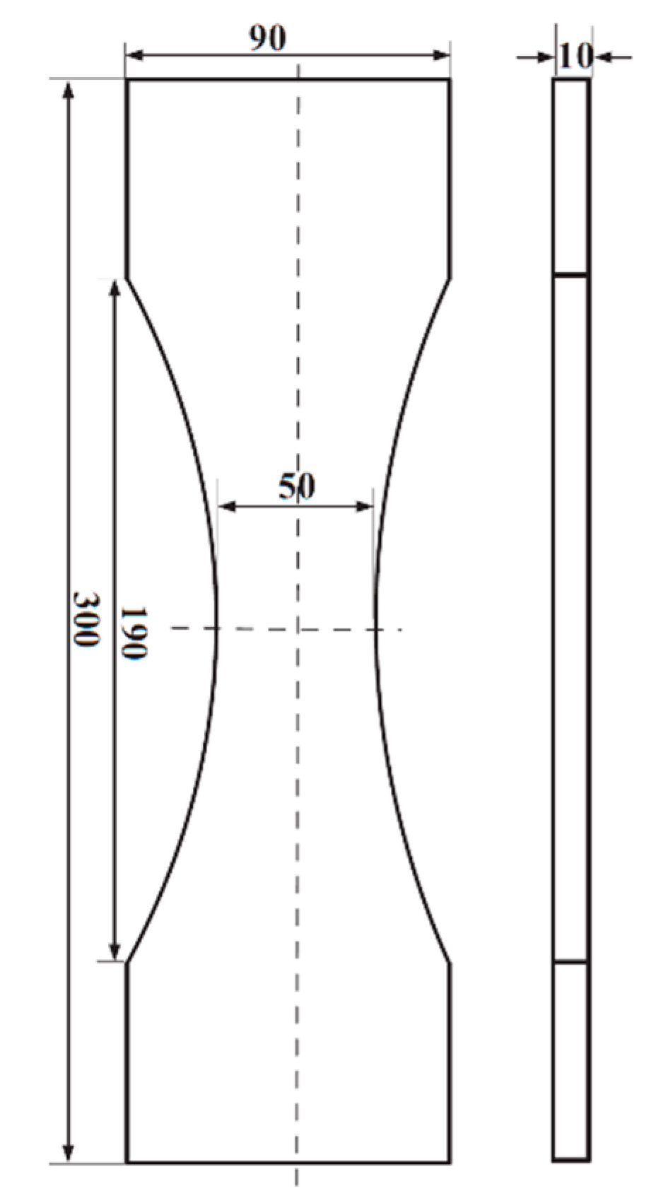
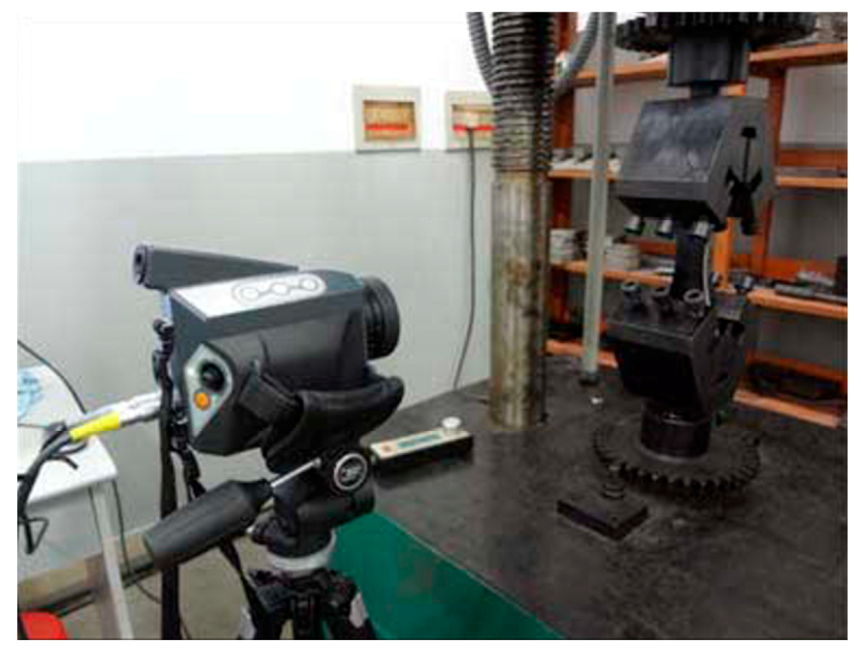
3. Experimental Details

Table 1. Chemical composition of AZ31B magnesium alloy (wt.%).

Mg	Al	Zn	Mn	Si	Ca	Cu	Fe	Ni
Bal.	2.8	0.7	0.4	0.1	0.04	0.01	0.005	0.001

shows the chemical composition of the experimental material, which is a typical commercial extruded AZ31B magnesium alloy sheet. Meanwhile, the thermophysical properties of AZ31B are given in

Table 2. Some thermophysical properties of AZ31B magnesium alloy.

Density, ρ (kg/m3)	Heat Capacity, C (J/(kg·K))	Thermal Conductivity, k (W/(m·K))
1770	1000	96

, where ρ, C, and k represent the density, specific heat capacity, and thermal conductivity, respectively. As we all know, extruded AZ31B magnesium alloy has significant anisotropy. The basic mechanical properties of AZ31B in both the extrusion and transverse directions are given in

Table 3. Tensile mechanical properties of AZ31B magnesium alloy.

Material	Tensile Strength, σm (MPa)	Yield Strength, σ0.2 (MPa)	Elongation at Failure, A (%)
Extrusion direction, ED	251	145	12
Transverse direction, TD	232	130	9

.

Hourglass-shaped specimens were selected in this study, the geometric dimensions of which are shown in Figure 1. The thickness of the specimen is 10 mm. The varying cross-sectional area will introduce a non-uniform stress distribution into the gauge of the specimen, which will be used to study the relationship between stress distribution and temperature distribution in the later section. The length of the gauge is 190 mm, in which the width of the specimen gradually transitions from 90 mm (at both ends, maximum cross-section) to 50 mm (at the center, minimum cross-section) in the form of a circular arc. Two types of specimens were prepared in this study, which are denoted as ED (extrusion direction) and TD (transverse direction). After being machined from the plate by spark-cutting, the specimens were smoothed with sandpapers of different grit. Black matte paint was evenly sprayed on the surface of the fatigue specimen with the purpose of increasing the thermal emission rate.

A high-frequency electromagnetic resonance fatigue testing machine (PLG-200D, Changchun New Testing Machine Co., Ltd., Changchun, Jilin Province, China) was employed in this study. The fatigue test was performed at room temperature with stress control mode. The load waveform was a sine wave. In addition, the load frequency was approximately 100 Hz. The stress ratio was chosen to be R = 0.1 (${\sigma }_{\min }/{\sigma }_{\max }$). Load levels were classified according to the maximum value of the nominal stress at the center of the specimen where the cross-sectional area is the smallest.

An infrared camera (InfraTec VarioCAM hr, InfraTec, Dresden, Saxony, Germany) was employed to real-timely record the surface temperature along with the ambient temperature during the fatigue test, as shown in Figure 2. The sampling speed of the camera was 50 frames per second. The temperature sensitivity is less than 0.08 K at 300 K. A companion software was used to generate raw thermographic data. The thermal image has a resolution of 384 × 288 and was stored in a special format. The infrared camera can thoroughly examine the entire surface of the specimen at each point (pixel by pixel). The spatial resolution is from 0.74 mm to 0.78 mm square pixels, depending on the scanner distance.

4. A Data-Processing Method for Eliminating External Heating

For fatigue research based on infrared thermography, only the temperature change caused by self-heating inside the material is related to fatigue damage [34]. If the temperature data is mixed with the influence of the boundary conditions, such as the temperature change of the fixture during the test, the results of the infrared thermography will be ambiguous [11,12]. An ideal boundary condition is to maintain a constant temperature at both ends of the specimen during the entire test. To achieve this ideal boundary condition, some researchers installed circulating cooling on the periphery of the fixture [27]. In this section, a data-processing method is proposed which can eliminate the influence of temperature changes on the boundary and achieve ideal boundary conditions.

4.1. One-Dimensional Heat Diffusion Model

The temperature change of the specimen during the fatigue test can be regarded as a one-dimensional heat conduction process, because the temperature change along the length direction is obvious and the temperature distribution along the width direction is basically uniform [25,26]. As described in Figure 3, the length of the specimen is recorded as the X-axis. The one-dimensional thermal diffusion equation can be obtained by averaging the temperature on each section of the specimen.

$$\rho C\left(\frac{\partial \stackrel{⁼}{\theta }}{\partial t}+\frac{\stackrel{⁼}{\theta }}{{\tau }^{1D}}\right)-k\left(\frac{{\partial }^2\stackrel{⁼}{\theta }}{\partial x^2}+\frac{1}{S}\frac{dS\partial \stackrel{⁼}{\theta }}{dx\partial x}\right)={\stackrel{⁼}{d}}_1$$

(6)

where $S\left(x\right)=e·w\left(x\right)$ represents the cross-section area of the specimen, e represents the thickness of the specimen, and $w\left(x\right)$ represents the width of the specimen at x. $\stackrel{⁼}{\theta }\left(x,t\right)$ represents the average temperature variation over the thickness-width obtained from the thermal image. The time constant ${\tau }^{1D}\left(x\right)=\frac{\rho CS\left(x\right)}{2h\left(e+w\left(x\right)\right)}$ represents the total heat exchange between the surface of the specimen and the surrounding environment. In particular, h is the comprehensive heat transfer coefficient on the surface, taking into account both the convection and radiative heat transfer. According to reference [30], the value of h is 30–100 W/(m²·K).

In addition to the governing equation given in Equation (6), the boundary conditions and initial conditions need to be specified. Then, the temperature evolution process of the specimen can be completely modeled. As shown in Figure 3, two virtual boundaries are set to limit the discussion of temperature changes to the middle portion of the specimen $-\frac{L}{2}$ ≤ x ≤ $\frac{L}{2}$. The boundary conditions of the model can be set as the temperature values on the two virtual boundaries, which are directly provided by the infrared thermal camera. If the temperature model takes the entire specimen as the object, the contact heat transfer between the specimen and the fixture acts as the boundary condition [29]. Modeling such boundary conditions will be cumbersome, because the temperature at both ends of the specimen needs to be measured which is clamped in the fixture. On the other hand, since the specimen is sufficiently cooled before cyclic loading, it can be considered that its temperature is uniform and consistent with the surrounding environment. The initial condition can be written as $\stackrel{⁼}{\theta }\left(x,t=0\right)=0$. Then, we have obtained a thermal diffusion model that can be used to describe the temperature change of the specimen during the fatigue test, as shown below:

$$\{\begin{array}{c}\rho C\left(\frac{\partial \stackrel{⁼}{\theta }}{\partial t}+\frac{\stackrel{⁼}{\theta }}{{\tau }^{1D}}\right)-k\left(\frac{{\partial }^2\stackrel{⁼}{\theta }}{\partial x^2}+\frac{1}{S}\frac{dS\partial \stackrel{⁼}{\theta }}{dx\partial x}\right)=s={\stackrel{⁼}{d}}_1\\ \stackrel{⁼}{\theta }\left(x,t=0\right)=0\\ \stackrel{⁼}{\theta }\left(x=\pm \frac{L}{2},t\right)={\stackrel{⁼}{\theta }}_{exp}\left(x=\pm \frac{L}{2},t\right)\end{array}$$

(7)

where s is the heat source term of the model. As explained before, the source term s is equal to the intrinsic dissipation when only the average temperature change is discussed. θ_exp is the actual temperature determined from the thermal image. L is the distance between the two boundaries.

In the work of Yang et al., the heat exchange through the lateral of the specimen was ignored [35]. This study adopts the same assumptions as Yang. In addition, the one-dimensional thermal diffusion model can be simplified to Equation (8).

$$\{\begin{array}{c}\rho C\frac{\partial \stackrel{⁼}{\theta }}{\partial t}-k\left(\frac{{\partial }^2\stackrel{⁼}{\theta }}{\partial x^2}+\frac{1}{S}\frac{dS\partial \stackrel{⁼}{\theta }}{dx\partial x}\right)={\stackrel{⁼}{d}}_1\\ \stackrel{⁼}{\theta }\left(x,t=0\right)=0\\ \stackrel{⁼}{\theta }\left(x=\pm \frac{L}{2},t\right)={\stackrel{⁼}{\theta }}_{exp}\left(x=\pm \frac{L}{2},t\right)\end{array}$$

(8)

4.2. Description of the Data-Processing Method

As a linear partial differential equation, Equation (8) can be divided into two parts that can be superimposed together [30]. This is the so-called superposition principle.

$$\stackrel{⁼}{\theta }\left(x,t\right)={\stackrel{⁼}{\theta }}_b\left(x,t\right)+{\stackrel{⁼}{\theta }}_d\left(x,t\right)$$

(9)

where

$$\{\begin{array}{c}\rho C\frac{\partial {\stackrel{⁼}{\theta }}_b}{\partial t}-k\left(\frac{{\partial }^2{\stackrel{⁼}{\theta }}_b}{\partial x^2}+\frac{1}{S}\frac{dS\partial {\stackrel{⁼}{\theta }}_b}{dx\partial x}\right)=0\\ {\stackrel{⁼}{\theta }}_b\left(x,t=0\right)=0\\ {\stackrel{⁼}{\theta }}_b\left(x=\pm \frac{L}{2},t\right)={\stackrel{⁼}{\theta }}_{exp}\left(x=\pm \frac{L}{2},t\right)\end{array}$$

(10a)

$$\begin{array}{c}\rho C\frac{\partial {\stackrel{⁼}{\theta }}_d}{\partial t}-k\left(\frac{{\partial }^2{\stackrel{⁼}{\theta }}_d}{\partial x^2}+\frac{1}{S}\frac{dS\partial {\stackrel{⁼}{\theta }}_d}{dx\partial x}\right)={\stackrel{⁼}{d}}_1\\ {\stackrel{⁼}{\theta }}_d\left(x,t=0\right)=0\\ {\stackrel{⁼}{\theta }}_d\left(x=\pm \frac{L}{2},t\right)=0\end{array}$$

(10b)

Because the heat source term of Equation (10a) is zero, it means that no heat is produced within the middle portion of the specimen. Therefore, θ_b represents a temperature profile, which only represents the temperature change caused by the boundary conditions. In contrast, the heat source distribution in Equation (10b) is the same as in the actual test, Equation (7), and its boundary conditions are always kept at zero throughout the thermal process. Therefore, θ_d only considers the contribution of the heat source distribution to the temperature change.

Equation (10b) can be obtained by subtracting Equation (10a) from Equation (9). The temperature distribution represented by Equation (10a) can be calculated by finite difference since the thermal boundary conditions can be extracted from the thermal image, which is known. Equation (9) can be obtained by modeling the thermal image data, which is also known. In this way, the temperature increase caused by the boundary conditions θ_b was successfully eliminated from the overall temperature increase θ. The remaining part is the temperature change only caused by the intrinsic dissipation inside the material θ_d.

5. Results and Discussion

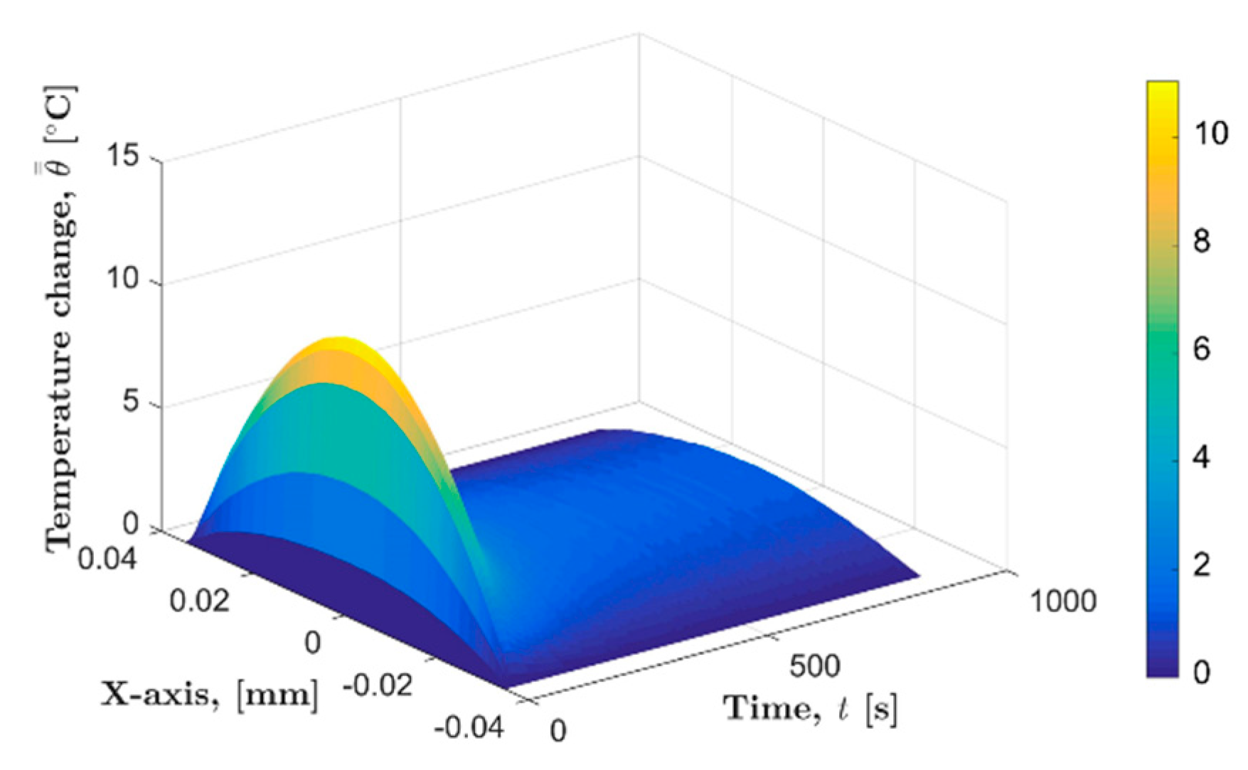
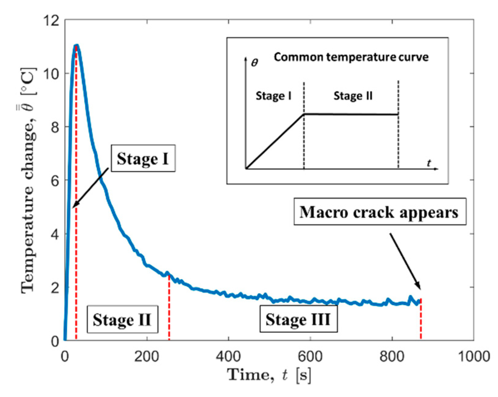
5.1. The Temperature Evolution after Processing

Figure 4 shows an example of the temperature evolution of the specimen after using the data processing to eliminate the influence of boundary conditions. This example was carried out with the specimen in the extrusion direction under a load of 145 MPa. $\stackrel{⁼}{\theta }=T-T_0$ represents the temperature increment.

Figure 5 is a typical center temperature evolution curve after eliminating external influence, which is extracted from the temperature data shown in Figure 4. This center temperature evolution curve can be divided into three stages: (I) the initial temperature rise stage, (II) the temperature drop stage, and (III) the temperature equilibrium temperature stage. In the process represented by the temperature evolution curve, the fatigue specimen is continuously subjected to the cyclic load, and the temperature rise of several degrees is maintained. Here we only consider the part before the macro crack appears. This is because the algorithm to eliminate external heating is based on a one-dimensional temperature model, which is built on a complete specimen. After the macro cracks appeared, the integrity of the specimen was destroyed. The one-dimensional thermal diffusion model is no longer applicable, and the proposed data-processing method also fails.

It is worth noting that the three-stage temperature evolution curve of AZ31B magnesium alloy is relatively rare in the published literature. The common temperature evolution curve reported in much of the literature contains only two stages [36], as shown in the label picture in the upper right corner of Figure 5. In 2009, Doudard et al. [13] found that the trend of the temperature evolution curve during fatigue test is related to the cyclic hardening/softening mode of the material. According to the work of Doudard et al. [13], the three-stage temperature evolution of AZ31B magnesium alloy is consistent with the temperature evolution curve of cyclic hardening materials under cyclic loading. Then, judging from the shape of the temperature evolution curve, AZ31B magnesium alloy should be cyclic hardening in this study. On the other hand, the common two-stage temperature evolution curve corresponds to a particular case of constant isotropic hardening, in which a steady mean temperature is reached just after the initial temperature rise. In this case, the global plastic strain energy, the global dissipated energy density per cycle, and the global stored energy per cycle all remain constant. It means that the fatigue heat production is always constant.

Three representatives are selected to analyze the spatial temperature distribution of the AZ31B magnesium alloy specimen. They are the temperature distribution profiles in the length direction of specimen at the moments of 50 s, 100 s, and 150 s, as shown in Figure 6. After using data processing to eliminate the influence of external heating, the temperature on both boundaries of the distribution profile is zero at the three selected moments. In fact, it can be seen from Figure 4 that the temperature data after processing always maintains zero temperature rise on the two boundary conditions throughout the test. This indeed achieves complete control of the boundary conditions, and the processed temperature data is equivalent to the test results obtained under ideal conditions where there is no fixture temperature rise.

Because of the symmetrical geometry of the specimen, the internal stress also presents a symmetrical distribution. The distribution of the internal heat source depends on the distribution of the internal stress. Therefore, the distribution of internal heat sources should also show symmetry [24]. The temperature evolution of an object is affected by both boundary conditions and internal heat distribution. When the temperature on the specimen boundary remains constant, the temperature change of the specimen during fatigue is completely affected by the internal heat source. Therefore, the entire temperature distribution of the specimen should also show symmetry, which is consistent with the symmetrical distribution of internal heat sources [6]. In Figure 6, the temperature profile located in the negative half axis of the X-axis is folded on the positive half axis, which is marked with a blue cross. The temperature profiles of the positive half axis and that of the negative half axis are in good agreement at the three selected moments, which indicates that the temperature profile curve presents a good symmetry. This is consistent with the theoretically predicted symmetry. The temperature distribution at many other times was also checked, involving tests carried out under different loads. The temperature distribution profiles after processing always showed good symmetry.

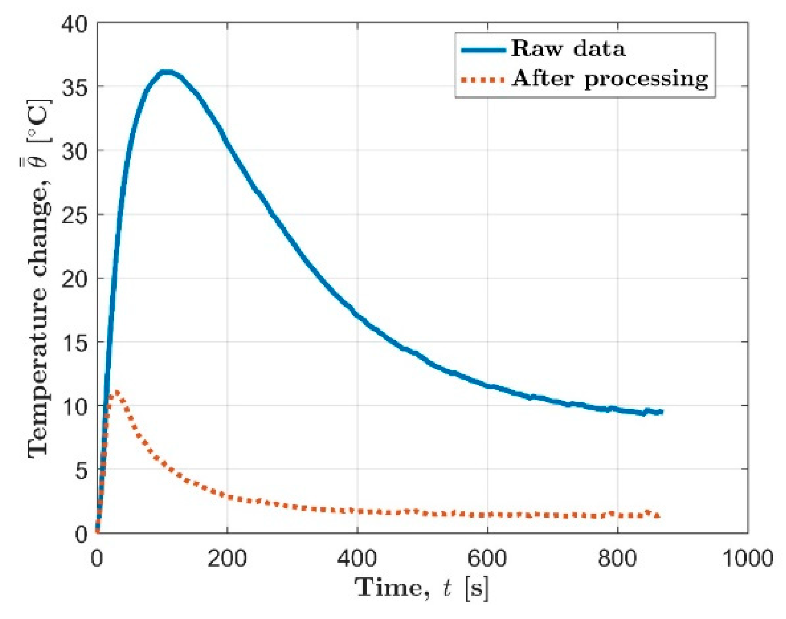
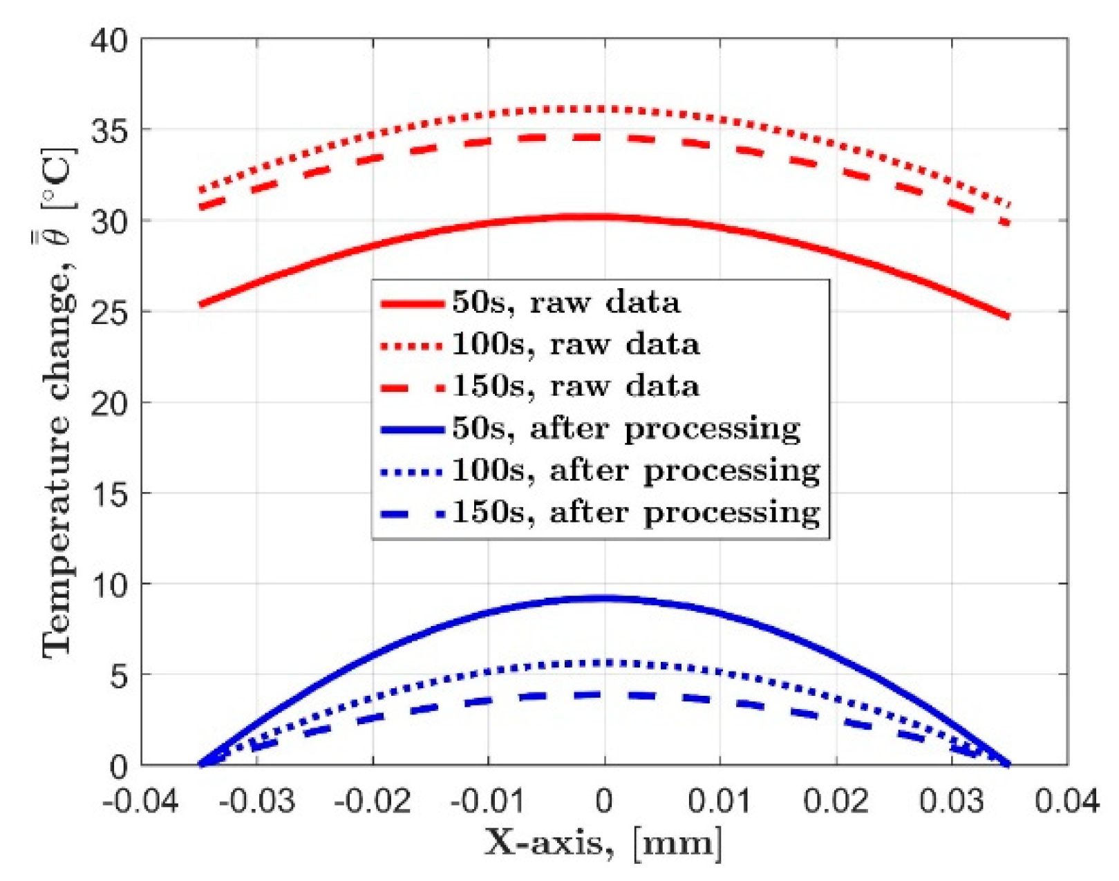
5.2. Significance of the Data Processing

A center temperature evolution curve before data processing is given in Figure 7, which corresponds to the example given in Figure 5. It is obvious that the temperature after processing is much lower than the temperature before processing. The temperature data after processing maintains the original internal heat source intensity and distribution, but the external heating has been removed. It reflects the temperature increase caused only by fatigue self-heating. A significant reduction in the temperature after eliminating the external heating indicates that a large portion of the temperature rise of the specimen in the raw data is caused by the heating from the fixture [37].

Figure 8 shows the raw temperature distribution profiles corresponding to the three selected moments in Figure 6. As in the case of the temperature evolution curve, the fatigue specimen has a higher temperature distribution at three selected moments before the external heating is eliminated by data-processing. Another point worth noting is that the temperature distribution profiles before processing does not show as good symmetry as those after processing. The temperature of the upper part of the specimen is higher. The temperature difference between the two boundaries is 0.47 °C, 0.81 °C and 0.88 °C at 50 s, 100 s, and 150 s, respectively. As mentioned before, the temperature distribution of the specimen should be symmetrical under ideal conditions. The inconsistency of heat loss at both ends of the specimen is a possible reason for the asymmetry of the temperature distribution profile before process. This proves once again that the boundary conditions have an influence on the temperature of the specimen [11,37].

Comparing the temperature evolution curve before and after the processing, it can be concluded that the raw temperature data obtained directly from the infrared camera is largely affected by external heating. The temperature rise caused by external heating is not related to fatigue damage of the material. When one wants to study the fatigue of a material based on its own heat production under fatigue, the temperature rise caused by external heating must be properly handled.

The data-processing method proposed in this paper effectively controls the boundary conditions and eliminates the asymmetries of temperature distribution due to the external heating. From a certain aspect, it is simple to use the proposed method to control external heating, because no additional cooling device is required on the fatigue testing machine. After the processing, the temperature increase of the specimen is only caused by the intrinsic dissipation inside the material, which can be used for subsequent fatigue studies.

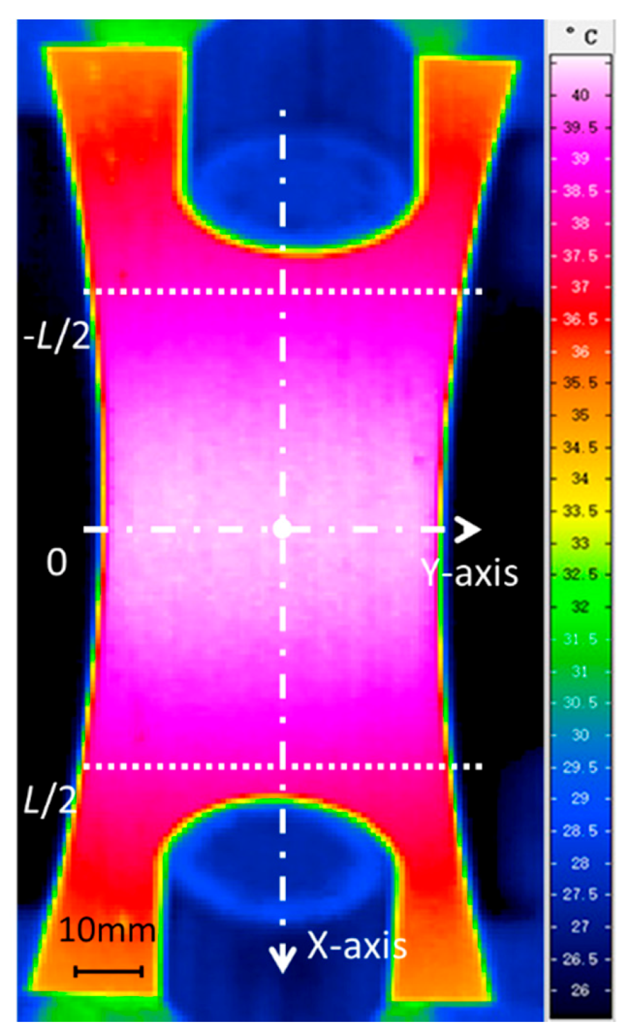
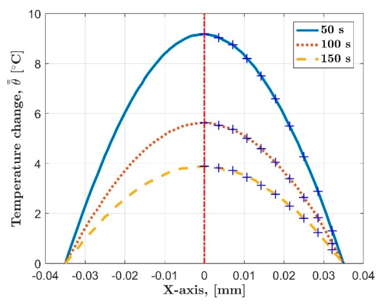
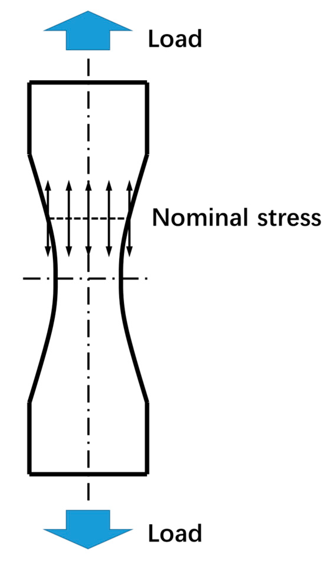
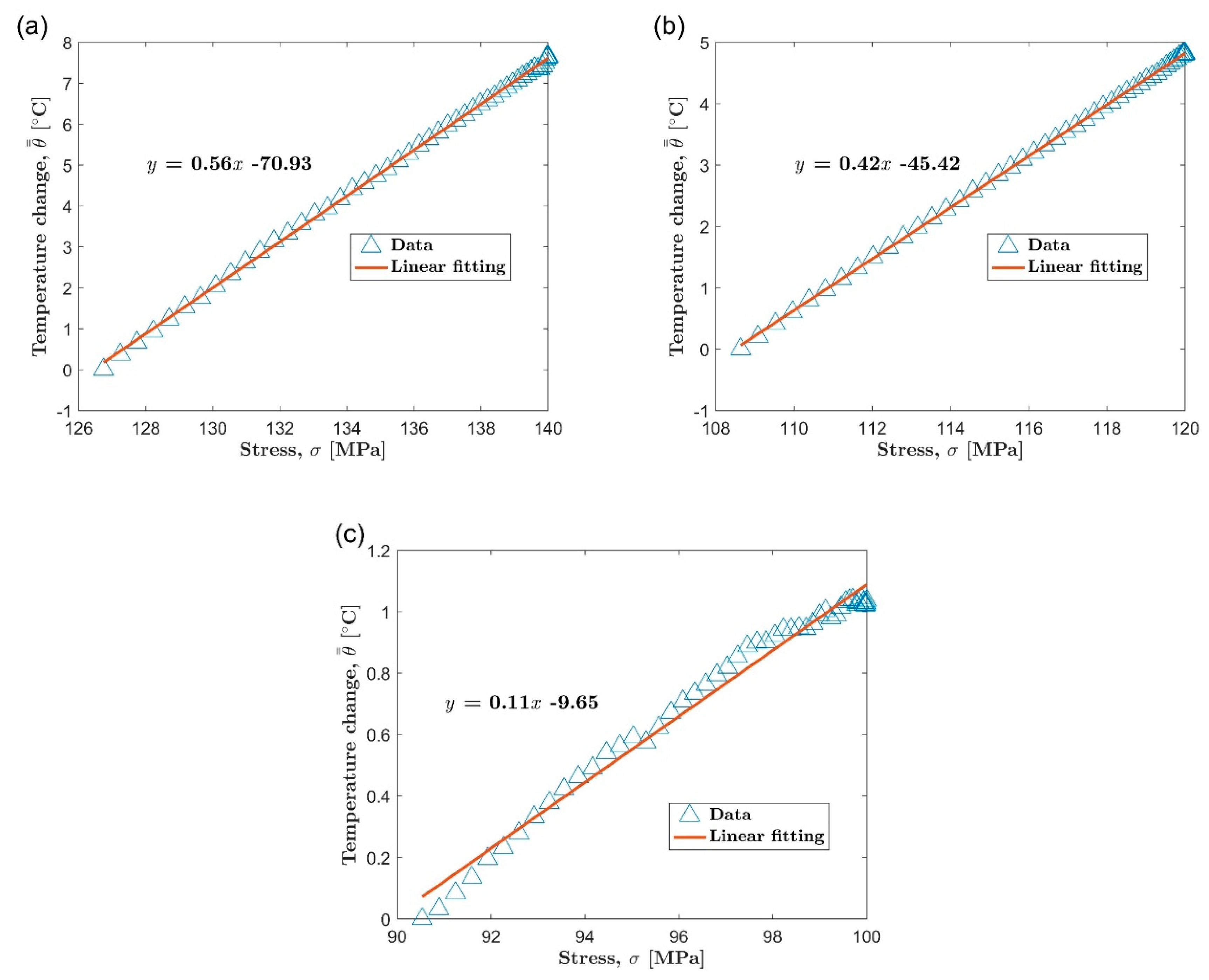
5.3. Relationship between Temperature Distribution and Stress Distribution

After zeroing the boundary conditions using the proposed data-processing method, the internal heat generation becomes the dominant factor determining the temperature of the specimen. The varying stress distribution along the length of the hourglass specimen will result in uneven distribution of the heat source, which will further affect the temperature distribution of the specimen [24,30]. In this section, we will analyze the relationship between stress distribution and temperature distribution.

Select the moment when the central temperature evolution curve reaches the maximum value to study the influence of the stress distribution, which is the critical point of the first initial temperature rise stage and the second temperature drop stage. There are two main reasons for choosing such a moment: first, the temperature change rate with time is zero at this moment, it means that the entire specimen is in a temporary thermal equilibrium state; second, at this time, there is a large temperature difference inside the specimen, which helps to overcome the influence of random noise.

Assume that the stresses on each section of the specimen are consistent, and determine the stress on each section of the specimen according to σ_A = F/S_A (the nominal stress), where σ_A represents the stress of cross-section A, F represents the applied tension, and S_A represents the area of the cross-section, as shown in Figure 9. Naturally, as the size of cross-section increases from the center to the end of the specimen, the stress on each section decreases continuously. Along the length of the specimen, the temperature and stress on each cross-section are matched one-to-one. In this way, we get the relationship curve of temperature and stress from the hourglass-type specimen, as shown in Figure 10. The location of temperature measurement of Figure 10 is the upper half of the fatigue specimen, starting from the center to the upper boundary −L/2 (see Figure 5).

It can be seen that there is a strong correlation between the temperature distribution on the specimen surface and the internal stress distribution. The temperature of each cross-section of the specimen goes up linearly with the local stress. As the stress increases, the area of the hysteresis loop representing the strain-strain relationship under cyclic loading also increases. It means greater viscosity and/or plastic deformation of the material. As a result, more mechanical work is converted into heat energy, which leads to a stronger heat source inside the material. Thus, for the hourglass specimen used in this study, the change of the cross-sectional area will lead to the internal heat source of the specimen to gradually decrease from the center position with higher local stress to the end of the lower local stress. Under the effect of heat conduction, the change of heat source distribution is smoothed to a certain extent. Finally, the temperature increases linearly with increasing local stress.

In general, the slope of the temperature-stress relationship line goes up with the increasing load level. In particular, the slope of the temperature-stress line will greatly increase when the applied load exceeds a certain critical value. As shown in Figure 11, the experimental results in both the extrusion direction and the transverse direction conform to this trend. The test was performed once at each stress level. The slope of the temperature-stress relationship line is small under lower load, and the slope of these lines become significantly larger as the increase of load level under higher load. The small slope means that the temperature distribution on the surface of the specimen under lower load is approximately uniform, and it is hardly affected by changes in the local stress. The large slope of temperature-stress curve under high load indicates that the varying stress in the specimen has a strong influence on the surface temperature distribution. In addition, this effect of stress distribution on temperature distribution is also stronger at higher load levels.

In our opinion, this sudden change in the slope of the temperature-stress relationship curve can be considered to be a manifestation of the alteration of intrinsic dissipative mechanism under fatigue loading [5,25]. Under the load below the fatigue limit, the intrinsic dissipation is dominated by viscoelasticity, and the self-heating inside the material is low. When the applied load is higher than the fatigue limit, self-heating begins to transform into plastic dissipation, and a large amount of heat is generated per unit time. Therefore, it should be possible to use the slope of the temperature-stress curve to assess the fatigue limit, just like using other existing thermal indicators of self-heating, such as the temperature at the equilibrium stage and the slope of initial temperature rise.

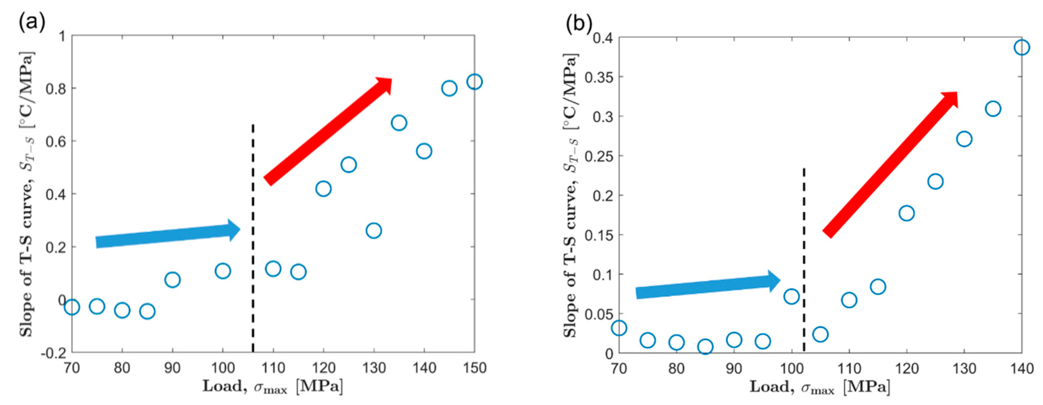
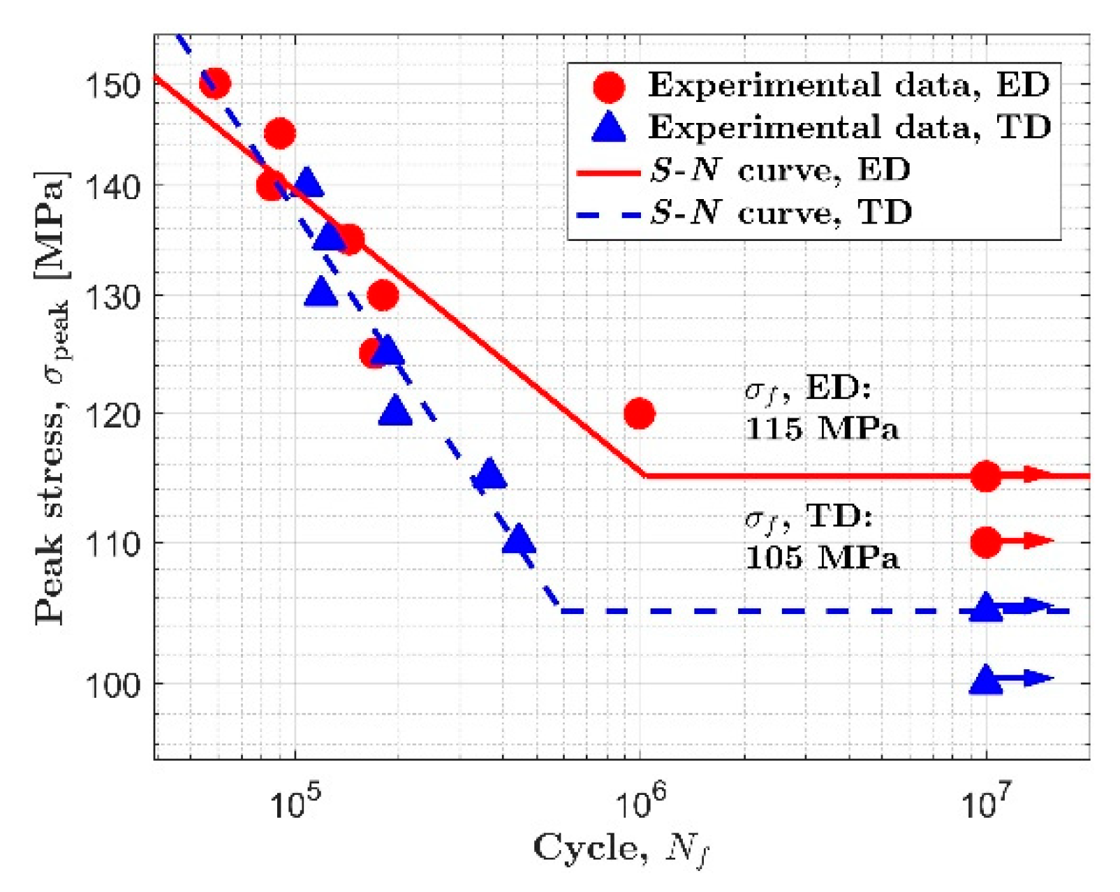
5.4. Fatigue Limit Assessment Based on the New Thermal Indicator

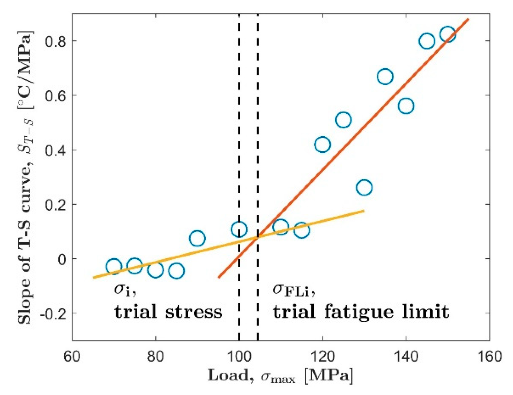
The purpose of this section is to verify whether the slope of the temperature-stress relationship curve can be used for fatigue limit assessment. Based on this newly proposed temperature indicator, three different algorithms (the classic Luong method [5], the iterative method [16] and the threshold method [11]) are used to estimate the fatigue limit of AZ31B magnesium alloy.

5.4.1. Luong Method

As one of the classic infrared thermographic methods for fatigue limit assessment, Luong method uses two straight lines to interpolate the temperature data above and below the fatigue limit, and the stress value corresponding to the intersection of the two straight lines is regarded as the fatigue limit [5].

The Luong method was applied to the temperature data in Figure 11, and the fatigue limit evaluation results are shown in Figure 12. The temperature data was separated according to the fatigue limit (the fatigue strength at 10⁷ cycles was defined as a fatigue limit) determined by the S-N curve in Figure 13. For the extrusion direction, the fatigue limit given by the Luong method is 101.46 MPa, and the fatigue limit is 108.24 MPa for the transverse direction.

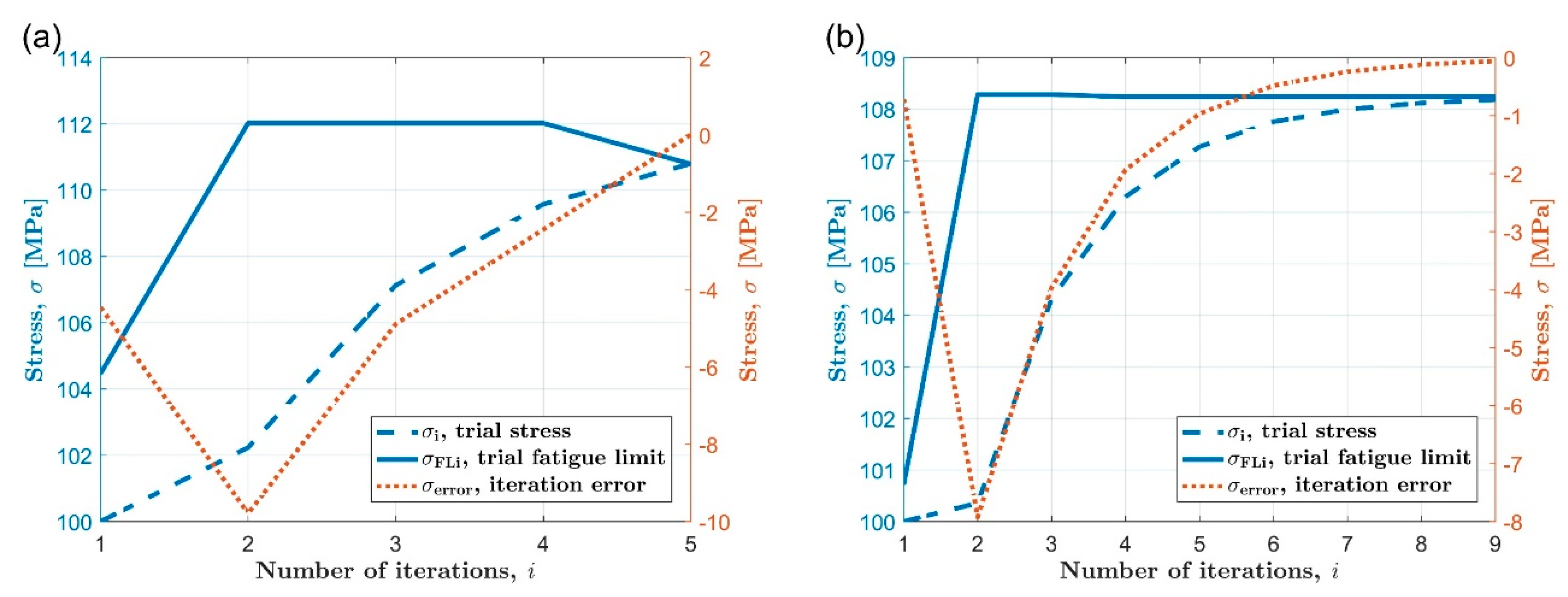
5.4.2. Iterative Method

In 2005, Curà et al. proposed and adopted an iterative process to calculate the fatigue limit [16]. This iterative method can automatically determine the fatigue limit of the material only based on the temperature data itself. It is different from the Luong method which requires the temperature data to be previously separated into two parts of above and below the fatigue limit. Here we will use the iterative method to calculate the fatigue limit which is also based on the temperature data indicated by the slope of the temperature-stress curve.

The iterative method requires multiple iterations to obtain the final fatigue limit. Taking the extrusion direction as an example, the main steps of fatigue limit assessment are given: First, 100 MPa is selected as the initial trial stress, and the temperature data is preliminarily divided into two groups higher than and lower than σ_i. Second, use two straight lines to fit the data that has been divided into the two temporary groups in the first step, respectively. Take the stress value corresponding to the intersection of the two fitted straight lines as the trial fatigue limit σ_FLi. Third, the difference between the trial stress and the trial fatigue limit is calculated and recorded as the iteration error σ_error. Figure 14 illustrates the first three steps of the iterative method to calculate the fatigue limit. The fourth step is to judge the iteration error. If the absolute value of the iteration error is greater than 0.1 MPa, correct the current trial stress according to σ_i+1 = σ_i – 0.5 × σ_error, and repeat the first to fourth steps. Until the iteration error is less than 0.1 MPa, stop the iteration and use the trial fatigue limit at this time as the final result of the evaluation.

In the calculation of the specimen in the transverse direction, the same parameters as the extrusion direction are selected, including the initial trial stress, and the error limit used to terminate the iteration. A MATLAB program developed by the author is used for the iterative calculation process.

The evaluation results of fatigue limit of AZ31B magnesium alloy in extrusion and transverse directions are shown in Figure 15. For the extrusion direction, the fatigue limit calculated according to the iterative method is 110.79 MPa. A total of 5 iterations have been experienced in the calculation process, and the maximum iteration error is close to −10MPa. On the other hand, it took 9 iterations to obtain the final fatigue limit of 108.24 MPa for the transverse direction, and the maximum iteration error is about −8 MPa. During the calculation of the fatigue limit, the changes of the three parameters (the trial stress, the trial fatigue limit and the iteration error) with the number of iterations are shown in Figure 16. For specimens in both directions, only a few iterations are needed to obtain the final evaluation results of the fatigue limit, which shows the high efficiency of the iterative method.

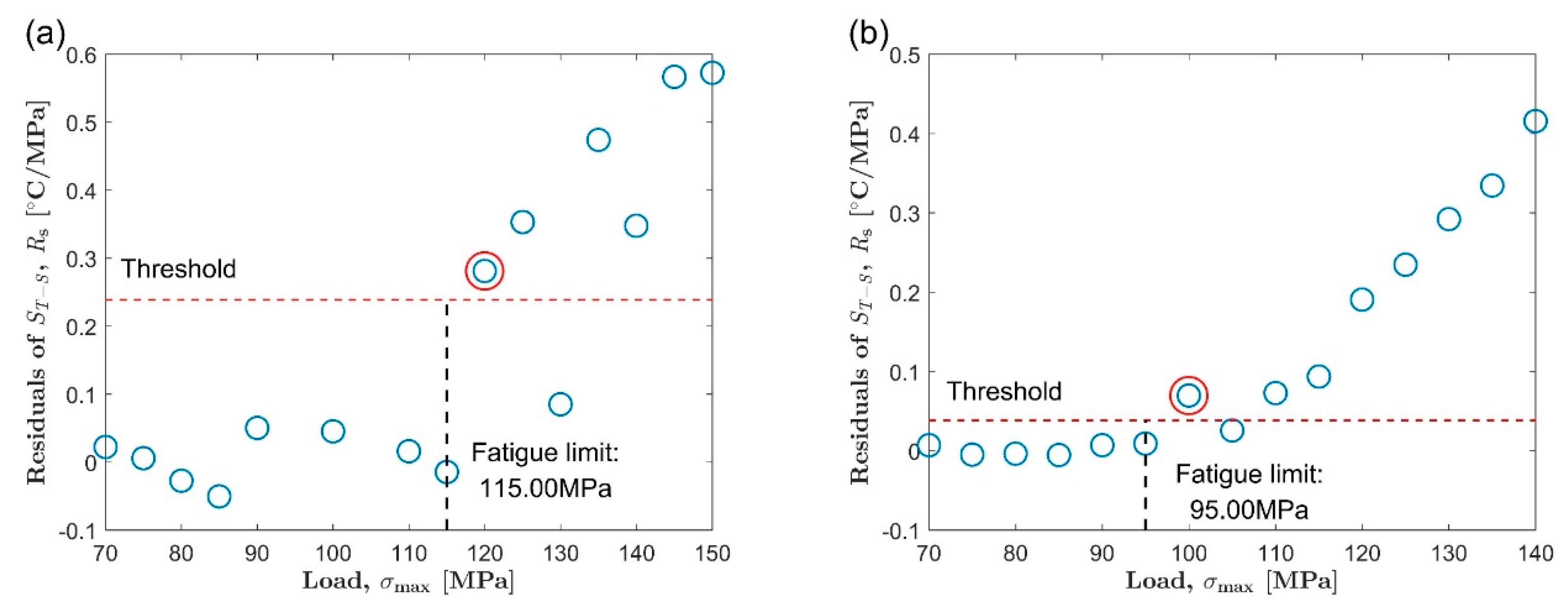
5.4.3. Threshold Method

In 2015, De Finis et al. proposed a robust analysis program to estimate the fatigue limit of stainless steel, which can be called the threshold method [11]. Same as the iterative method, the threshold method also does not require a border to divide temperature data before the assessment, and is also a fatigue limit estimation method that can be automatically implemented.

The threshold method includes the following main steps:

First, starting from the lowest load level, successively select 5 temperature data under lower load. It should be ensured that these data points are within the load range less than the fatigue limit.

Second, use the least square method to linearly fit the selected 5 temperature data, and get the regression line.

Third, calculate the residual error of each temperature data to the regression line.

Fourth, perform robust analysis on all residuals obtained in the third step to obtain the standard deviation of these residuals.

Fifth, set 6 times the standard deviation calculated in the fourth step as the threshold.

Sixth, starting from the sixth data (exclude the first 5 points used for fitting in the first step), check the temperature data under each load level one by one from low to high. In addition, record the load level corresponding to the first temperature data whose residual error exceeds the threshold, such as σ_N. At last, the load level σ_N-1 before σ_N is recognized as the final fatigue limit.

The threshold method was used to process the temperature data represented by the slope of the temperature-stress curve in Figure 11, and the fatigue limit evaluation results are shown in Figure 17. The red dashed line represents the threshold determined in the fifth step. The first data point that exceeds the threshold (the sixth step) is marked with a red circle. For the extrusion direction, the fatigue limit estimated by the threshold method is 115 MPa. For the transverse direction, the fatigue limit is 95 MPa.

5.4.4. Discussion of Results

The evaluation results of fatigue limit of AZ31B magnesium alloy are summarized in

Table 4. Summarized results of fatigue limit obtained based on different thermal indicators.

No.	Thermal Indicator	Material	Method	σtherm (MPa)	Method	σsta (MPa)	Error (%)	Ref.
1	TS *	AZ31B, ED	Luong	101.46	S-N	115	11.77	-
2	TS	AZ31B, TD	Luong	108.24	S-N	105	3.09	-
3	TS	AZ31B, ED	Iteration	110.79	S-N	115	3.66	-
4	TS	AZ31B, TD	Iteration	108.24	S-N	105	3.09	-
5	TS	AZ31B, ED	Threshold	115	S-N	115	0	-
6	TS	AZ31B, TD	Threshold	95	S-N	105	9.52	-
7	PT *	XC55	Luong	374	Staircase	399	6.27	[5]
8	PT	ASTM A 182 F6NM	Luong	138.9	Staircase	169.3	17.96	[11]
9	PT	17-4 PH	Luong	205	Staircase	212.1	3.35	[11]
10	PT	Fe 510	Iteration	199	Staircase	203	1.97	[16]
11	PT	ASTM A 182 F6NM	Threshold	140	Staircase	169.3	17.31	[11]
12	PT	17-4 PH	Threshold	201.7	Staircase	212.1	4.90	[11]
13	IT *	Fe 510	Iteration	210	Staircase	203	3.45	[16]
14	IT	Duplex A890 Grade 4A	Threshold	128.33	Goodman modified	122	5.19	[12]
15	IT	AISI 316	Threshold	66.67	Dixon	64.58	3.24	[12]
16	IT	17-4 PH	Threshold	211.67	Staircase	212	0.16	[12]

* TS: Slope of temperature-stress line. PT: Plateau temperature. IT: Initial temperature rise slope.

. These results come from three different fatigue limit algorithms, but all are based on the slope of the temperature-stress line. For comparison, Table 4 also shown the fatigue limit evaluation results based on two common thermal indicators, the plateau temperature and the initial temperature rise slope. These results are quoted from published literature.

Compared with the result of the traditional S-N curve method, the maximum error of all six evaluation results based on the slope of the temperature-stress line is 11.77%, and the average value of the error is 5.19%. For the results based on the thermal indicator of plateau temperature, the maximum error with traditional statistical methods is 17.96%, and the average value of the error is 8.63%. The thermographic method based on the initial temperature rise slope has a maximum error of 5.19% and an average value of 3.01%. The error of the thermographic method relative to the traditional statistical method is calculated according to the following formula:

$$Eorrer=\left|\frac{{\sigma }_{therm}-{\sigma }_{sta}}{{\sigma }_{sta}}\right|\times 100\%$$

where σ_therm represents the fatigue limit calculated by thermographic methods and σ_sta represents the fatigue limit calculated by statistical methods.

Compared with the accuracy of the thermographic method using common thermal indicators, the thermographic method based on the slope of the temperature-stress line shows a satisfactory result for the evaluation of the fatigue limit of AZ31B magnesium alloy. Therefore, at least for this study, it is reasonable to trust that the slope of the temperature-stress line can be taken as a new thermal indicator which reflects the relationship between the self-heating and load levels under fatigue, and can be used in infrared thermographic to evaluate the fatigue limit.

It should be emphasized that this new thermal indicator is determined according to the surface temperature distribution of the specimen. This is significantly different from the commonly used thermal indicators, such as the temperature at the equilibrium stage and the initial temperature rise slope, which are calculated based on the temperature change at the specimen center over time. The temperature distribution analysis was selected to be carried out when the temperature of the specimen reached the highest value. It makes that the proposed thermal indicator can be obtained through surface temperature analysis at the early stage of fatigue loading. Because the temperature evolution curve will quickly reach the maximum after the fatigue test begins. Therefore, it is not necessary to continuously apply cyclic load to the specimen until the final fatigue failure. This will save a lot of test time. In future work, we plan to conduct research on other materials. In particular, those materials with different temperature evolution trends.

6. Conclusions

In this article, infrared thermographic technique was employed to analyze the temperature change of AZ31B magnesium alloy under cyclic load, and on this basis, the fatigue limit of AZ31B was evaluated.

A data-processing method designed to eliminate external influences has been proposed, which is based on the principle of mathematical superposition. The proposed data-processing method can control the boundary conditions, which can be confirmed by the always zero temperature rise on the two boundaries. After processing, the temperature rise of the specimen is dominated by the self-heating inside the material, which causes the temperature distribution along the length to show good symmetry. From a certain aspect, it is simple to use the proposed method to control external heating, because no additional cooling device is required on the fatigue testing machine.

The changing cross-sectional area will lead to a not uniform stress distribution inside the hourglass specimen. Based on the temperature data after processing, a significant linear relationship was found between the local temperature and the local stress on each cross-section of the specimen. Under lower load, the slope of this temperature-stress relationship line is smaller, indicating that the temperature distribution is hardly affected by the stress distribution. However, under a larger load, the slope of the temperature-stress relationship line is larger, indicating that the stress distribution greatly affects the temperature distribution.

The slope of the temperature-stress relationship line goes up as the load level increases. When a certain critical load is exceeded, the slope of the temperature-stress line will greatly increase. This sudden change can be considered to be induced by the alteration of intrinsic dissipative mechanism. Using the slope of the temperature-stress relationship line as a new thermal indicator, three different algorithms all yielded satisfactory results for fatigue limit evaluation of AZ31B magnesium alloy. This was true for the AZ31B magnesium alloy in both extrusion and transverse directions.

References

1. Fontanari, V.; Benedetti, M. Fatigue Design and Defects in Metals and Alloys. Metals 2020, 10, 865. [Google Scholar] [CrossRef]
2. De Finis, R.; Palumbo, D.; Serio, L.; De Filippis, L.; Galietti, U. Correlation between Thermal Behaviour of Aa5754-H111 during Fatigue Loading and Fatigue Strength at Fixed Number of Cycles. Materials 2018, 11, 719. [Google Scholar] [CrossRef] [Green Version]
3. Khonsari, M.M.; Amiri, M. Introduction to Thermodynamics of Mechanical Fatigue; CRC Press: New York, NY, USA, 2013. [Google Scholar]
4. Zhang, H.X.; Wu, G.H.; Yan, Z.F.; Guo, S.F.; Chen, P.D.; Wang, W.X. An experimental analysis of fatigue behavior of Az31B magnesium alloy welded joint based on infrared thermography. Mater. Des. 2014, 55, 785–791. [Google Scholar] [CrossRef]
5. Luong, M.P. Fatigue Limit Evaluation of Metals Using an Infrared Thermographic Technique. Mech. Mater. 1998, 28, 155–163. [Google Scholar] [CrossRef]
6. Guo, S.; Zhou, Y.; Zhang, H.; Yan, Z.; Wang, W.; Sun, K.; Li, Y. Thermographic Analysis of the Fatigue Heating Process for Az31B Magnesium Alloy. Mater. Des. (1980–2015) 2015, 65, 1172–1180. [Google Scholar] [CrossRef]
7. Connesson, N.; Maquin, F.; Pierron, F. Dissipated Energy Measurements as a Marker of Microstructural Evolution: 316L and Dp600. Acta Mater. 2011, 59, 4100–4115. [Google Scholar] [CrossRef]
8. Wang, X.G.; Crupi, V.; Jiang, C.; Guglielmino, E. Quantitative Thermographic Methodology for Fatigue Life Assessment in a Multiscale Energy Dissipation Framework. Int. J. Fatigue 2015, 81, 249–256. [Google Scholar] [CrossRef]
9. Wang, X.G.; Crupi, V.; Guo, X.L.; Zhao, Y.G. Quantitative Thermographic Methodology for Fatigue Assessment and Stress Measurement. Int. J. Fatigue 2010, 32, 1970–1976. [Google Scholar] [CrossRef]
10. Luong, M.P. Infrared Thermographic Scanning of Fatigue in Metals. Nucl. Eng. Des. 1995, 158, 363–376. [Google Scholar] [CrossRef] [Green Version]
11. De Finis, R.; Palumbo, D.; Ancona, F.; Galietti, U. Fatigue Limit Evaluation of Various Martensitic Stainless Steels with New Robust Thermographic Data Analysis. Int. J. Fatigue 2015, 74, 88–96. [Google Scholar] [CrossRef]
12. De Finis, R.; Palumbo, D.; Da Silva, M.M.; Galietti, U. Is the Temperature Plateau of a Self-Heating Test a Robust Parameter to Investigate the Fatigue Limit of Steels with Thermography? Fatigue Fract. Eng. Mater. Struct. 2018, 41, 917–934. [Google Scholar] [CrossRef]
13. Crupi, V. An Unifying Approach to Assess the Structural Strength. Int. J. Fatigue 2008, 30, 1150–1159. [Google Scholar] [CrossRef]
14. Fan, J.; Guo, X.; Wu, C. A New Application of the Infrared Thermography for Fatigue Evaluation and Damage Assessment. Int. J. Fatigue 2012, 44, 1–7. [Google Scholar] [CrossRef]
15. La Rosa, G.; Risitano, A. Thermographic Methodology for Rapid Determination of the Fatigue Limit of Materials and Mechanical Components. Int. J. Fatigue 2000, 22, 65–73. [Google Scholar] [CrossRef]
16. Cura, F.; Curti, G.; Sesana, R. A New Iteration Method for the Thermographic Determination of Fatigue Limit in Steels. Int. J. Fatigue 2005, 27, 453–459. [Google Scholar] [CrossRef]
17. Zhang, L.; Liu, X.S.; Wu, S.H.; Ma, Z.Q.; Fang, H.Y. Rapid Determination of Fatigue Life based on Temperature Evolution. Int. J. Fatigue 2013, 54, 1–6. [Google Scholar] [CrossRef]
18. Liakat, M.; Khonsari, M.M. An Experimental Approach to Estimate Damage and Remaining Life of Metals Under Uniaxial Fatigue Loading. Mater. Des. 2014, 57, 289–297. [Google Scholar] [CrossRef]
19. Liakat, M.; Khonsari, M.M. Rapid Estimation of Fatigue Entropy and Toughness in Metals. Mater. Des. (1980–2015) 2014, 62, 149–157. [Google Scholar] [CrossRef]
20. Yan, Z.F.; Zhang, H.X.; Wang, W.X.; He, X.L.; Liu, X.Q. Temperature Evolution in Magnesium Alloy During Static and Cyclic Loading. Mater. Sci. Tech. Lond. 2014, 30, 1229–1234. [Google Scholar] [CrossRef]
21. Curà, F.; Gallinatti, A.E.; Sesana, R. Dissipative Aspects in Thermographic Methods. Fatigue Fract. Eng. Mater. Struct. 2012, 35, 1133–1147. [Google Scholar] [CrossRef]
22. Meneghetti, G. Analysis of the Fatigue Strength of a Stainless Steel Based on the Energy Dissipation. Int. J. Fatigue 2007, 29, 81–94. [Google Scholar] [CrossRef]
23. Meneghetti, G.; Ricotta, M.; Atzori, B. A Two-Parameter, Heat Energy-Based Approach to Analyse the Mean Stress Influence on Axial Fatigue Behaviour of Plain Steel Specimens. Int. J. Fatigue 2016, 82, 60–70. [Google Scholar] [CrossRef]
24. Doudard, C.; Calloch, S.; Hild, F.; Roux, S. Identification of Heat Source Fields From Infrared Thermography: Determination of ‘Self-Heating’ in a Dual-Phase Steel by Using a Dog Bone Sample. Mech. Mater. 2010, 42, 55–62. [Google Scholar] [CrossRef] [Green Version]
25. Guo, Q.; Guo, X.; Fan, J.; Syed, R.; Wu, C. An Energy Method for Rapid Evaluation of High-Cycle Fatigue Parameters Based On Intrinsic Dissipation. Int. J. Fatigue 2015, 80, 136–144. [Google Scholar] [CrossRef]
26. Guo, Q.; Guo, X. Research on High-Cycle Fatigue Behavior of Fv520B Stainless Steel Based on Intrinsic Dissipation. Mater. Des. 2016, 90, 248–255. [Google Scholar] [CrossRef]
27. Facchinetti, M.; Florin, P.; Doudard, C.; Calloch, S. Identification of Self-Heating Phenomena Under Cyclic Loadings Using Full-Field Thermal and Kinematic Measurements: Application to High-Cycle Fatigue of Seam Weld Joints. Exp. Mech. 2015, 55, 681–698. [Google Scholar] [CrossRef]
28. Huang, J.; Pastor, M.; Garnier, C.; Gong, X. Rapid Evaluation of Fatigue Limit on Thermographic Data Analysis. Int. J. Fatigue 2017, 104, 293–301. [Google Scholar] [CrossRef] [Green Version]
29. Chrysochoos, A.; Louche, H. An Infrared Image Processing to Analyse the Calorific Effects Accompanying Strain Localisation. Int. J. Eng. Sci. 2000, 38, 1759–1788. [Google Scholar] [CrossRef]
30. Blanche, A.; Chrysochoos, A.; Ranc, N.; Favier, V. Dissipation Assessments during Dynamic very High Cycle Fatigue Tests. Exp. Mech. 2015, 55, 699–709. [Google Scholar] [CrossRef]
31. Boulanger, T.; Chrysochoos, A.; Mabru, C.; Galtier, A. Calorimetric Analysis of Dissipative and Thermoelastic Effects Associated with the Fatigue Behavior of Steels. Int. J. Fatigue 2004, 26, 221–229. [Google Scholar] [CrossRef]
32. Wong, A.K.; Jones, R.; Sparrow, J.G. Thermoelastic constant or thermoelastic parameter. J. Phys. Chem. Solids 1987, 48, 749–753. [Google Scholar] [CrossRef]
33. Risitano, A.; Risitano, G. Cumulative damage evaluation of steel using infrared thermography. Theor. Appl. Fract. Mec. 2010, 54, 82–90. [Google Scholar] [CrossRef]
34. Berthel, B.; Chrysochoos, A.; Wattrisse, B.; Galtier, A. Infrared image processing for the calorimetric analysis of fatigue phenomena. Exp. Mech. 2008, 48, 79–90. [Google Scholar] [CrossRef]
35. Yang, W.; Guo, X.; Guo, Q.; Fan, J. Rapid Evaluation for High-Cycle Fatigue Reliability of Metallic Materials through Quantitative Thermography Methodology. Int. J. Fatigue 2019, 124, 461–472. [Google Scholar] [CrossRef]
36. Doudard, C.; Calloch, S. Influence of Hardening Type on Self-Heating of Metallic Materials under Cyclic Loadings at Low Amplitude. Eur. J. Mech. A/Solids 2009, 28, 233–240. [Google Scholar] [CrossRef]
37. Bouache, T.; Pron, H.; Caron, D. Identification of the Heat Losses at the Jaws of a Tensile Testing Machine. Exp. Mech. 2016, 56, 287–295. [Google Scholar] [CrossRef]
Figure 1. Geometric dimensions of the specimen (mm).
Metals 10 01331 g001
Figure 2. Infrared camera and fatigue testing machine.
Metals 10 01331 g002
Figure 3. Modeling the temperature change process of the specimen.
Metals 10 01331 g003
Figure 4. Surface temperature evolution of the specimen after process.
Metals 10 01331 g004
Figure 5. A typical center temperature evolution curve after data processing.
Metals 10 01331 g005
Figure 6. Temperature distribution profiles after processing at three different moments.
Metals 10 01331 g006
Figure 7. Center temperature evolution curve before and after process.
Metals 10 01331 g007
Figure 8. Comparison of temperature distribution profiles before and after processing.
Metals 10 01331 g008
Figure 9. Nominal stress on each section.
Metals 10 01331 g009
Figure 10. Temperature and stress relationship curves, AZ31B magnesium alloy extrusion direction: (a) 140 MPa, (b) 120 MPa, (c) 100 MPa.
Metals 10 01331 g010
Figure 11. The slope of temperature vs. stress curve at different stress levels: (a) extrusion direction, ED, (b) transverse direction, TD.
Metals 10 01331 g011
Figure 12. Fatigue limit evaluation by using Luong method: (a) extrusion direction, ED and (b) transverse direction, TD.
Metals 10 01331 g012
Figure 13. Fatigue limits obtained from S-N curve.
Metals 10 01331 g013
Figure 14. The iterative method for evaluating fatigue limit.
Metals 10 01331 g014
Figure 15. Fatigue limit evaluation by using the iterative method: (a) extrusion direction, ED and (b) transverse direction, TD.
Metals 10 01331 g015
Figure 16. Change of iteration error in the process of fatigue limit calculation: (a) extrusion direction, ED and (b) transverse direction, TD.
Metals 10 01331 g016
Figure 17. Fatigue limit evaluation by using the threshold method: (a) extrusion direction, ED and (b) transverse direction, TD.
Metals 10 01331 g017