Adaptive Finite Element Prediction of Fatigue Life and Crack Path in 2D Structural Components

Abstract

The existence of a hole near a growing fatigue crack can cause the crack trajectory to deviate. Unless the hole is too close to the crack, the crack is arrested at the edge of the hole and does not progress further. The purpose of this paper was to predict the crack propagation and lifetime of two-dimension geometries for linear elastic materials in mixed-mode loading using a finite element source code program written in Visual Fortran language. The finite element mesh is generated using the advancing front method. The onset criterion of crack propagation was based on the equivalent stress intensity factor which provides the most important parameter that must be accurately estimated for the mixed-mode loading condition. The maximum circumferential stress theory was used as a direction criterion. The modified compact tension (MCTS) was studied to demonstrate the influence of the hole’s presence on the direction of crack growth and fatigue life for different configurations. The Paris’ law model has been employed to evaluate the mixed-mode fatigue life for MCTS in different configurations under the linear elastic fracture mechanics (LEFMs) assumption. The framework involves a progressive crack extension study of stress intensity factors (SIFs), crack growth direction, and fatigue life estimation. The results show that the fatigue growth was attracted to the hole either changes its direction to reach the hole or floats by the hole and grows as the hole is missed. The results of the study agree with several crack propagation experiments in the literature revealing similar crack propagation trajectory observations.

1. Introduction

To maintain an acceptable level of durability over the entire operational time, the fatigue crack growth in engineering structures should be monitored. Many experimental methods are used today to study the propagation of cracks in steel plates. Nevertheless, most of the experimental approaches to find an effective solution are destructive, expensive, and time-consuming. To overcome these challenges, scientists have proposed several analytical and finite element techniques to quickly find final solutions [1,2,3]. The structures and components are fractured in many fields of engineering due to the accumulation of fatigue failure. Fatigue has therefore been widely studied [4,5,6]. Several studies have been conducted to date to investigate the interaction between cracks and holes. The finite element method (FEM) research has been shown to offer a reliable justification for experimental dynamic crack propagation in two-dimensional situations. If a crack trajectory is associated with a hole, it has first been found that it avoids the hole with a dynamic load and falls into the hole loaded by a similar quasi-static one [7]. The stress intensity factors (SIFs) describe the intensity of the singular stress fields and are, at the same time, a measure of the amount of the displacements in the crack area, i.e., they are also a measure for crack opening or the relative displacements of the crack surfaces. The SIFs depend on many parameters which are the applied loading of the component, the crack geometry or crack length/depth, the crack position, crack arrangement, the geometry of the component, and the type and location of the load application. Numerical analyses, such as finite element analysis, have become an incredibly useful method for modeling a crack’s propagation and determining fracture parameters such as the stress intensity factors and energy release rate. Over the last few decades, improvements to the finite element method have been continuously made in order to improve the handling of complex material models and experimental conditions. In the meantime, new approaches and methods in several areas of study have been suggested and developed rapidly, including the Finite Element Method (FEM), Discrete Element Method (DEM) [8,9,10], Element-Free Galerkin (EFG) method [11], Extended Finite Element Method (XFEM) [12,13], cohesive element method [14] and phase field method [15].

The practical importance of fracture mechanics applications relies on SIFs. Numerical analyses using the FEM usually computes first-order energy derivatives related to crack length or equivalent SIFs to propagate a crack gradually in small, controlled straight-line growth increments. The advantages and disadvantages of using finite elements in computational mechanics have been extensively addressed [16]. De Oliveira Miranda and Meggiolaro et al. study the problem of mesh refining and related errors in computing SIFs using the FEM [16,17]. It was noticed that too much mesh refinement in crack problems could significantly improve the accuracy of the calculation when increasing the computational time. The development of the present software began in 2004 and has continued to add a range of features from version to version for the simulation of two-dimensional fatigue crack growth with the under the LEFM assumptions [18,19,20,21,22,23,24,25]. LEFMs apply when the material’s nonlinear deformation is limited to a small area at the tip of the crack, whereas Elastic Plastic Fracture Mechanics (EPFMs) is proposed to analyze the relatively large plastic zones and assumes isotropic and elastic-plastic materials. The energy fields of the strain or the opening displacement near the crack tips are determined based on the assumption. If the energy or opening exceeds the critical value, the crack grows. The fracture is modeled by the splitting node approach [3] and the trajectory follows the successive linear extensions of each crack increment. The propagation process is driven by a linear elastic fracture mechanics (LEFMs) approach with minimum user interaction. In 3D modeling, the re-meshing strategy presents a number of important additional computational challenges compared to a 2D analysis. However, the predicted values of stress intensity factors in both 2D and 3D were almost identical with the same degree of mesh refinement [26]. The developed source code is a finite element software that yields results comparable with the results obtained from the currently available commercial software in fracture analysis. Concerning knowledge, commercial software is not suitable for at least two reasons: first, it does not completely understand the basic algorithm that it uses, and second there is a complete lack of the state-of-the-art programming skills in its development. The efficiency of the proposed program was demonstrated in many cases such as a compact tension specimen under mixed-mode loading [3], specimen with a hole at its center and three interacting cracks [25], modified four-points bend specimen [22], modified compact tension specimen [6], two internal noncolinear cracks [18] and polymethyl methacrylate (PMMA) specimen with three holes [18].

2. Materials and Methods

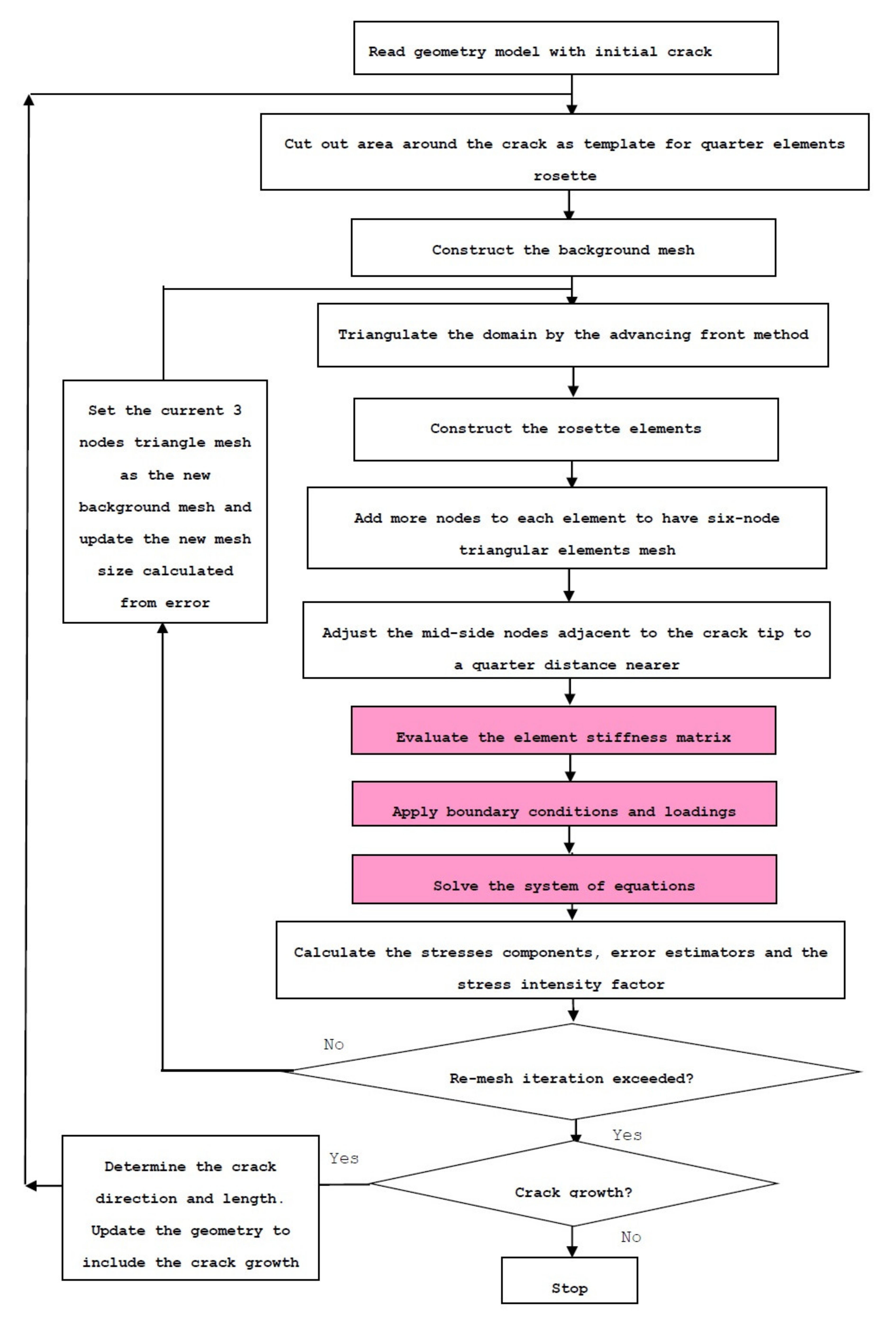
2.1. Program Development Procedure

The finite element process usually comprises three main elements—pre-processing, processing, and post-processing. The processing is the most time-consuming part of computing because it involves the evaluation and assembly processes of the stiffness matrices equations and the solver method. The developed code is a simulation program for the assessment of 2D crack propagation processes under conditions of LEFMs. Using the finite element (FE) process, this program predicts the growth of quasi-static fatigue crack in 2D components taking into consideration the mechanical boundary conditions of the fracture. For the crack trajectory simulation, four essential components are used for the adaptive mesh FE analysis, namely, the mesh optimization algorithm, the crack criterion, the direction criterion, and the crack propagation methodology. The mesh refining can be managed by each element’s characteristic scale, predicted according to the error estimator. An incremental theory with the Von Mises yield criterion is applied to this initial model. After each load stage is over, the solution errors are calculated. When the error reaches a stated cumulative error at some point in the course of the experiment, the incremental analysis is disrupted and a new FE model is created. The system decides whether to configure the mesh automatically. The system refines the mesh when necessary, within the original boundary conditions. The solution variables (displacement, stresses, strains, etc.) are mapped from the old mesh into the new mesh after it is created. The analysis is then restarted and continues until the errors are again greater than the pre-decided number.

Users may display their responses through a graphical post-processor in the final analysis or at each stage. The crack criterion is employed to assess the start of the cracks. In LEFM, the SIFs are typically used as a criterion for fracture. The directional criteria are the third part of a crack growth simulation using an adaptive mesh in the FE strategy. The direction criterion is also used to determine the direction of the crack’s growth. Several methods are used for predicting the direction of a crack’s path, including maximum circumferential stress theory, maximum energy release theory, and minimum strain-energy density theory. An FE model is defined at each stage of crack growth. In the first step, the model is provided as an input for the simulation. The output of the algorithm itself is then generated by the models provided in the previous stages. At each step, as the crack grows, the elements within the geometry are deleted and rebuilt with an adaptive strategy and modified for the next propagation process. Figure 1 displays the computational procedure that is used to model fatigue crack growth. The main steps of this procedure are explained in detail by [22] and [23].

2.2. Adaptive Mesh Refinements and Crack Growth Criteria

The computational efficiency is highly dependent on numerous parameters, such as the mesh density, mesh refinement, and the number of cracks. During each modeling stage, conventional progressive fracture simulation algorithms update the model geometry with a short straight-line crack forward segment. The direction of each straight, linear growth segment can be determined with a linear elastic 2D model, implying a guideline of growth direction and defining two parameters that characterize a Williams stress field of the first-order near the tip of the crack. These two parameters are the symmetrical first-order mode I and the anti-symmetrical mode II—SIFs (K_I, K_II). Adaptive re-meshing strategies for subsets add each segment of the crack’s advance by modifying the existing mesh of FEs. It takes place in the region before the present crack tip to remove elements and nodes and replace them with smaller elements along the crack faces that must be added. Usually, these updated elements provide a small standardized element rosette in the current crack tip position. During each modeling stage, only a geometrical representation of a crack path must be modified because the cracks are not specifically depicted in an adaptive network. This direct method has been extended to represent multiple cracks without refining the meshes between successive crack tips [27].

The maximum circumferential stress theory [28] states that cracks grow in a direction normal to the maximum tangential tensile stress for isotropic materials under mixed-mode loading.

The tangential stress in polar coordinates is given by:

$${\sigma }_{\theta }=\frac{1}{\sqrt{2\pi r}}\cos \frac{\theta }{2}\left[K_I{\cos }^2\frac{\theta }{2}-\frac{3}{2}{K}_{II}\sin \theta \right]$$

(1)

By solving $d{\sigma }_{\theta }/d\theta =0$ for $\theta$ to get the direction normal to the maximum tangential stress, the solution is given by:

$$K_I\sin \theta +K_{II}\left(3\cos \theta -1\right)=0$$

(2)

which can be solved as:

$$\theta =\pm {\cos }^{-1}\left\{\frac{3K_{II}^2+K_I\sqrt{K_I^2+8K_{II}^2}}{K_I^2+9K_{II}^2}\right\}$$

(3)

The sign ${\theta }_0$ must be reversed to the sign of $K_{II}$ to guarantee the maximum stress associated with the crack increment [29]. The two alternatives are seen in Figure 2.

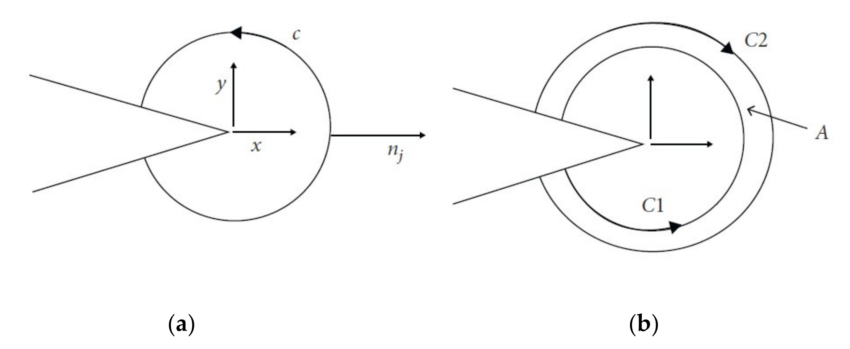
2.3. Stress Intensity Factors Method

The most successful engineering application of fracture mechanics is in the use of crack propagation laws based on stress intensity factor ranges [30]. It was developed by Irwin in the mid-1950s [31]. The stress intensity factor, denoted by K, was defined by Irwin as a mechanical parameter that characterizes the state of stress at a crack point. Numerous analytical solutions for the SIFs have been developed for a variety of common crack configurations. However, these analytical solutions are limited to simple crack geometries and loading conditions [32,33]. The implementation of small-sized yield criteria [34], which established a J-integral approach for studying the nonlinear behavior of the material. For FE analyses, the equivalent domain integral technique replaces the finite-size domain with a divergence theorem by integration along the contour.

The trajectory integral independent contour is as follows:

$$J={\displaystyle \underset{C}{\int }(W{n}_1}-{\sigma }_{ij}{n}_j\frac{\partial u_i}{\partial x})ds$$

(4)

where W is the strain-energy density, ${\sigma }_{ij}$ are the stresses, u_i is the local i axis displacement, s is the contour arc length, n_j is the outward unit normal to the contour C around the crack tip (Figure 3a).

For two-dimensional structures, the contour integral i is replaced by the area integral (Figure 3b). Then, Equation (4) is modified as:

$$J_k=-{\displaystyle \underset{A}{\int }}\left[W\frac{\partial q}{\partial x}-{\sigma }_{ij}\frac{\partial u_i}{\partial x}\frac{\partial q}{\partial x}\right]dA-{\displaystyle \underset{A}{\int }}\left[\frac{\partial W}{\partial x}-\frac{\partial }{\partial x}\left({\sigma }_{ij}\frac{\partial u_i}{\partial x}\right)\right]qdA-{\displaystyle \underset{s}{\int }{t}_i\frac{\partial u_i}{\partial x}qds}$$

(5)

For both modes I and II, Equation (5) simplify the calculation of mode I and II of SIFs but fails to calculate K_I and K_II separately for multiple load conditions. The integral to be considered in these situations is the following [35]:

$$J_k=-{\displaystyle \underset{A}{\int }}\left[W\frac{\partial q}{\partial x_k}-{\sigma }_{ij}\frac{\partial u_i}{\partial x_k}\frac{\partial q}{\partial x_j}\right]dA-{\displaystyle \underset{A}{\int }}\left[W\frac{\partial q}{\partial x_k}-{\sigma }_{ij}\frac{\partial }{\partial x_j}\left(\frac{\partial u_i}{\partial x_k}\right)\right]qdA-{\displaystyle \underset{s}{\int }{t}_i\frac{\partial u_i}{\partial x_k}qds}$$

(6)

where k denotes the index of the crack tip. Two possible methods can be used to calculate the SIFs. The first method is through interactions between the J-integral and the SIFs:

$$\begin{array}{l}{J}_1=\frac{\kappa +1}{8\mu }(K_I^2+K_{II}^2)\\ J_2=-\frac{\kappa +1}{4\mu }{K}_I{K}_{II}\end{array}$$

(7)

The second strategy uses the relation between SIFs and J₁ and J₂:

$$\begin{array}{l}{K}_I=0.5\sqrt{\frac{8\mu }{\kappa +1}}+(\sqrt{J_1-J_2}+\sqrt{J_1+J_2})\\ K_{II}=0.5\sqrt{\frac{8\mu }{\kappa +1}}+(\sqrt{J_1-J_2}-\sqrt{J_1+J_2})\end{array}$$

(8)

2.4. Adaptive Mesh Refinement

The optimization scheme in the field of FE mesh is the adaptive mesh refinement. This scheme is reliant on an a posteriori error estimator that is derived from the previous mesh generation. The estimator of the error in the mesh refinement is the stress error norm which is known as relative stress norm error. The h-type adaptive mesh optimization was used to derive the ratio of element norm stress error with the whole area’s average standard stress error. The size of the mesh for each element in this scheme is presented as:

$$h_e=\sqrt{2A_e}$$

(9)

where A_e is the triangle element area. For each element, the norm stress error is represented by:

$$\begin{array}{l}{‖e‖}_e^2={\displaystyle {\int }_{{\Omega }^e}{\left(\sigma -{\sigma }^{*}\right)}^{\mathrm{T}}\left(\sigma -{\sigma }^{*}\right)\mathrm{d}\Omega }\\ ={\displaystyle {\int }_{{\Omega }^e}{\left(\left\{\begin{array}{c}{\sigma }_x\\ {\sigma }_y\\ {\tau }_{xy}\\ {\sigma }_z\end{array}\right\}-\left\{\begin{array}{c}{\sigma }_x^{*}\\ {\sigma }_y^{*}\\ {\tau }_{xy}^{*}\\ {\sigma }_z^{*}\end{array}\right\}\right)}^{\mathrm{T}}\left(\left\{\begin{array}{c}{\sigma }_x\\ {\sigma }_y\\ {\tau }_{xy}\\ {\sigma }_z\end{array}\right\}-\left\{\begin{array}{c}{\sigma }_x^{*}\\ {\sigma }_y^{*}\\ {\tau }_{xy}^{*}\\ {\sigma }_z^{*}\end{array}\right\}\right)\mathrm{d}\Omega }\end{array}$$

(10)

Although, the average norm stress error over the whole domain is represented as:

$$\begin{array}{l}{‖ \mathrm{e} ^‖}^2=\frac{1}{m}{\displaystyle \sum _{e=1}^m{\displaystyle {\int }_{{\Omega }^e}{\sigma }^{\mathrm{T}}\sigma \mathrm{d}\Omega }}\\ =\frac{1}{m}{\displaystyle \sum _{e=1}^m{\displaystyle {\int }_{{\Omega }^e}{\left\{\begin{array}{c}{\sigma }_x\\ {\sigma }_y\\ {\tau }_{xy}\\ {\sigma }_z\end{array}\right\}}^{\mathrm{T}}\left\{\begin{array}{c}{\sigma }_x\\ {\sigma }_y\\ {\tau }_{xy}\\ {\sigma }_z\end{array}\right\}\mathrm{d}\Omega }}\end{array}$$

(11)

where m is the overall number of elements in the entire domain and ${\sigma }^{*}$ is the smoothed stress vector. The integration with the triangular isoparametric dimension will be converted in the FEM by the summation of quadratics according to the Radau rules as follows:

$$\begin{array}{cc}\hfill & {∥\mathrm{e}∥}_e^2={\underset{-1}{\overset{1}{\int }}\underset{-1}{\overset{1}{\int }}\left(\left\{\begin{array}{c}\sigma {\left(\xi ,\eta \right)}_x\\ \sigma {\left(\xi ,\eta \right)}_y\\ \tau {\left(\xi ,\eta \right)}_{xy}\\ \sigma {\left(\xi ,\eta \right)}_z\end{array}\right\}-\left\{\begin{array}{c}\sigma {\left(\xi ,\eta \right)}_x^{*}\\ \sigma {\left(\xi ,\eta \right)}_y^{*}\\ \tau {\left(\xi ,\eta \right)}_{xy}^{*}\\ \sigma {\left(\xi ,\eta \right)}_z^{*}\end{array}\right\}\right)}^{\mathrm{T}}\left(\left\{\begin{array}{c}\sigma {\left(\xi ,\eta \right)}_x\\ \sigma {\left(\xi ,\eta \right)}_y\\ \tau {\left(\xi ,\eta \right)}_{xy}\\ \sigma {\left(\xi ,\eta \right)}_z\end{array}\right\}-\left\{\begin{array}{c}\sigma {\left(\xi ,\eta \right)}_x^{*}\\ \sigma {\left(\xi ,\eta \right)}_y^{*}\\ \tau {\left(\xi ,\eta \right)}_{xy}^{*}\\ \sigma {\left(\xi ,\eta \right)}_z^{*}\end{array}\right\}\right)t^{e}det{J}^{e}d\xi d\eta \hfill \\ \hfill & ={\sum _{p=1}^3\left(\left\{\begin{array}{c}\sigma {\left({\xi }_p,{\eta }_p\right)}_x\\ \sigma {\left({\xi }_p,{\eta }_p\right)}_y\\ \tau {\left({\xi }_p,{\eta }_p\right)}_{xy}\\ \sigma {\left({\xi }_p,{\eta }_p\right)}_z\end{array}\right\}-\left\{\begin{array}{c}\sigma {\left({\xi }_p,{\eta }_p\right)}_x^{*}\\ \sigma {\left({\xi }_p,{\eta }_p\right)}_y^{*}\\ \tau {\left({\xi }_p,{\eta }_p\right)}_{xy}^{*}\\ \sigma {\left({\xi }_p,{\eta }_p\right)}_z^{*}\end{array}\right\}\right)}^{\mathrm{T}}\left(\left\{\begin{array}{c}\sigma {\left({\xi }_p,{\eta }_p\right)}_x\\ \sigma {\left({\xi }_p,{\eta }_p\right)}_y\\ \tau {\left({\xi }_p,{\eta }_p\right)}_{xy}\\ \sigma {\left({\xi }_p,{\eta }_p\right)}_z\end{array}\right\}-\left\{\begin{array}{c}\sigma {\left({\xi }_p,{\eta }_p\right)}_x^{*}\\ \sigma {\left({\xi }_p,{\eta }_p\right)}_y^{*}\\ \tau {\left({\xi }_p,{\eta }_p\right)}_{xy}^{*}\\ \sigma {\left({\xi }_p,{\eta }_p\right)}_z^{*}\end{array}\right\}\right)t^{e}det{J}^e{W}_p\hfill \end{array}$$

(12)

and similarly

$${‖ \hat{\mathrm{e}}‖}^2=\frac{1}{m}{\displaystyle \sum _{e=1}^m{{\displaystyle \sum _{p=1}^3\left(\left\{\begin{array}{c}\sigma {\left({\xi }_p,{\eta }_p\right)}_x\\ \sigma {\left({\xi }_p,{\eta }_p\right)}_y\\ \tau {\left({\xi }_p,{\eta }_p\right)}_{xy}\\ \sigma {\left({\xi }_p,{\eta }_p\right)}_z\end{array}\right\}\right)}}^{\mathrm{T}} \left(\left\{\begin{array}{c}\sigma {\left({\xi }_p,{\eta }_p\right)}_x\\ \sigma {\left({\xi }_p,{\eta }_p\right)}_y\\ \tau {\left({\xi }_p,{\eta }_p\right)}_{xy}\\ \sigma {\left({\xi }_p,{\eta }_p\right)}_z\end{array}\right\}\right)t^e\det J^e{W}_p}$$

(13)

where $t^e$ is the thickness of the element for a plane stress case and $t^e=1$ is the plane strain case. Consequently, the relative stress norm error ${\zeta }_e$ for each item is considerably less than 5%, which is acceptable for many applications in engineering [23]. Thus,

$${\zeta }_e=\frac{{‖e‖}_e}{‖\widehat{e}‖}\le \zeta$$

(14)

and the new element relative stress error level is identified as a permissible error by:

$${\epsilon }_e=\frac{{‖e‖}_e}{\zeta ‖\widehat{e}‖}\le 1$$

(15)

This means each element with ${\epsilon }_e>1$ is required to be refined and the new size of the mesh needs to be expected. Here the asymptotic convergence rate criteria are implemented, which presumes:

$${‖e‖}_e\propto h_e^p$$

(16)

where p is the approximation of polynomial order. In this study, P = 2 since the quadratic polynomial is used for the calculation of FEs. Thus, the new element estimated size is:

$$h_N=\frac{1}{\sqrt{{\epsilon }_e}}{h}_e$$

(17)

The existing mesh will be considered as the new background mesh and the advancing front method will be replicated depending on the user’s set number of mesh refinement.

2.5. Fatigue Crack Growth Analysis

As fatigue is a cyclical energy dissipation in the form of hysteretic loops, it is a cyclical damage process. The time elapsed for damage is represented by the number of fatigue cycles (N). This process is defined by crack growth per cycle (da/dN) which depends on the applied stress intensity factor range. In order to achieve fatigue crack growth, the resulting stress intensity range must exceed the threshold stress intensity factor at each crack tip, defined as:

$$\Delta K_{th}=f\Delta {\sigma }_{th}\sqrt{\pi a}$$

(18)

where f is a function of geometry and loading and $\Delta {\sigma }_{th}$ is the stress range limit. Equation (18) set a criterion whereby fatigue crack does not propagate if $\Delta \sigma <\Delta {\sigma }_{th}$. However, a parameter known as the equivalent stress intensity factor range, $\Delta K_{eq}$, is used as an indicator for fatigue crack propagation. In such $\Delta K_{eq} >\Delta K_{th}$ indicates that fatigue crack grows will happen otherwise there is no fatigue crack propagation.

Table 1. Commonly used $\Delta K_{eq}$ models.

Model Proposed by Authors	$\mathit{\Delta }{\mathit{K}}_{\mathit{e}\mathit{q}} \mathbf{Expression}$
(Tanaka 1974) [36]	$\Delta K_{eq}={(\Delta K_I^2+2\Delta K_{II}^2)}^{\raisebox{1ex}{$1$}\!\left/ \!\raisebox{-1ex}{$2$}\right.}$
(Tanaka 1974) [36]	$\Delta K_{eq}={(\Delta K_I^4+8\Delta K_{II}^4)}^{\raisebox{1ex}{$1$}\!\left/ \!\raisebox{-1ex}{$4$}\right.}$
(Lee, Y et al. 2005) [30]	$\Delta K_{eq}=\sqrt{\Delta K_1^2+\Delta K_{II}^2}$
(Xiangqiao, Shanyi et al. 1992) [37]	$\Delta K_{eq}=\frac{1}{2}\cos (\raisebox{1ex}{$\theta $}\!\left/ \!\raisebox{-1ex}{$2$}\right.)\left[\Delta K_I(1+\cos \theta )-3\Delta K_{II}sin\theta \right]$
(Richard, Buchholz et al. 2003; Richard, Schramm et al. 2014) [38]	$\Delta K_{eq}=\frac{\Delta K_I}{2}+\frac{1}{2}\sqrt{\Delta K_I^2+4(1.155\Delta K_{II}^2}$
(Demir, Ayhan et al. 2017) [39]	$\Delta K_{eq}={(1.0519\times K_I^4-0.035\times K_{II}^4+2.3056\times K_I^2\times K_{II}^2)}^{1/2}$
(Erdogan and Sih 1963) [28]	$\Delta K_{eq}=\cos \frac{\theta }{2}\left[K_I{\cos }^2\frac{\theta }{2}-\frac{3}{2}{K}_{II}\sin \theta \right]$

summarizes some of the common models used (proposed by the authors).

Predicting fatigue crack growth by using equivalent SIF ($\Delta K_{eq}$) is still the most commonly used method for dynamic loading structures. Using a modified form of Paris’ law, a power law is introduced for the association of the rate of propagation of fatigue crack and the corresponding SIF [36], which is given as:

$$\frac{da}{dN}=C{\left(\Delta K_{eq}\right)}^m$$

(19)

The fatigue life cycles can be estimated with Equation (19) for a crack increment Δa as:

$$\underset{0}{\overset{\Delta a}{{\displaystyle \int }}}\frac{da}{C{\left(\Delta K_{eq}\right)}^m}=\underset{0}{\overset{\Delta N}{{\displaystyle \int }}}dN=\Delta N$$

(20)

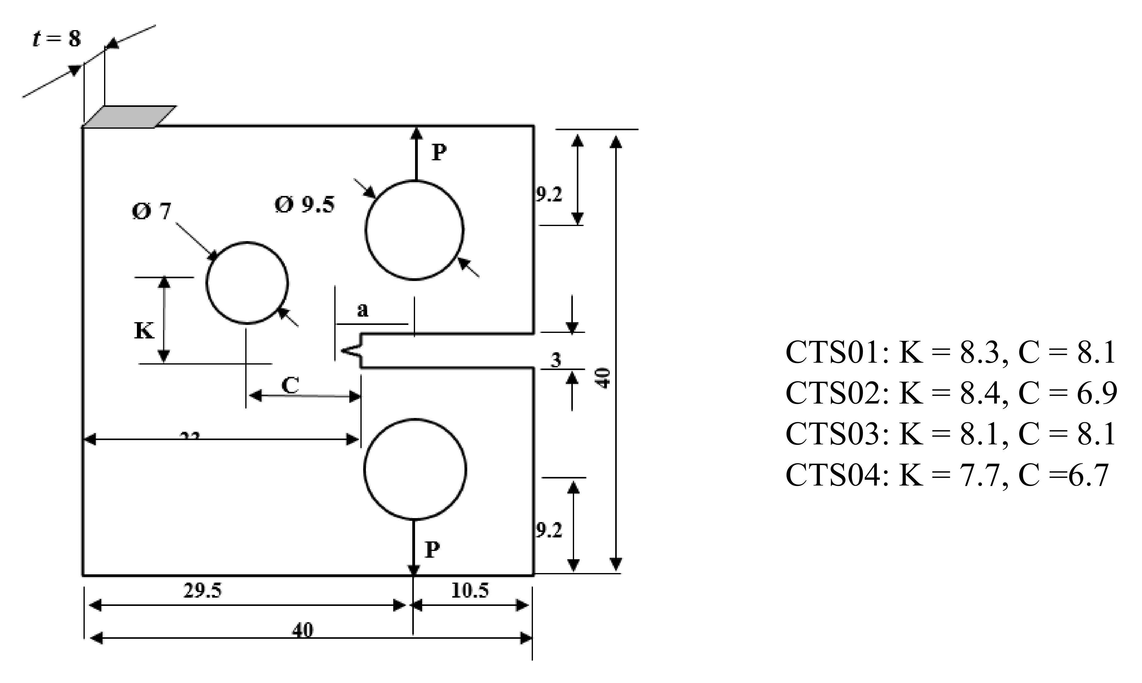
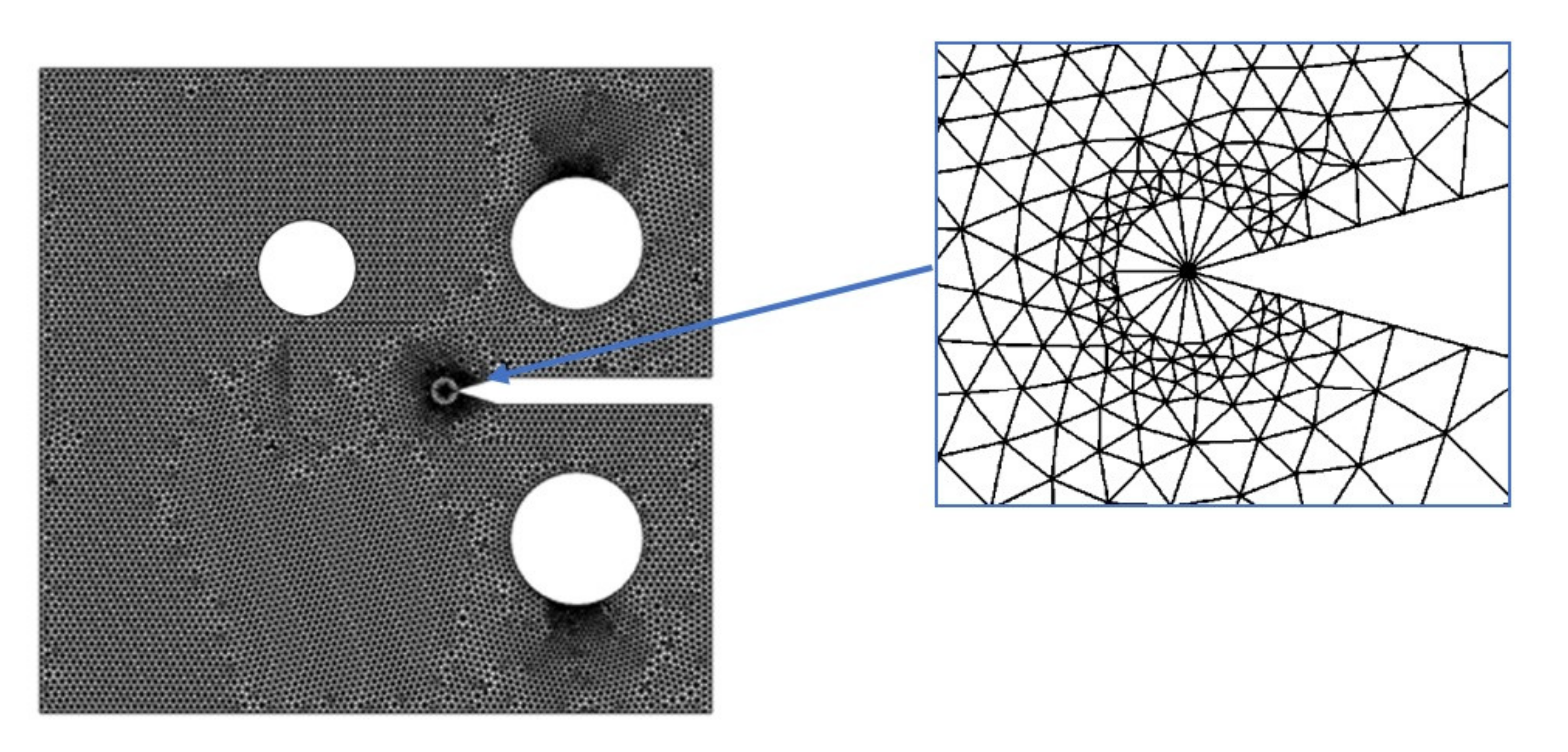
3. Numerical Results and Discussion

To demonstrate the ability of the developed program to predict fatigue crack growth and fatigue life, an MCTS with different hole positions is used. The dimensions of this geometry with various configurations is shown in Figure 4. The diameter of the third hole is 7 mm, located from the crack tip as seen in Figure 4, at horizontal and vertical distances K and C, respectively. The material properties are elastic modulus E = 205 GPa, Poisson’s ratio υ = 0.29, yield strength σ_y = 285 MPa, and ultimate strength σ_u = 491 MPa. The Paris’ law coefficient C = 8.59 × 10⁻¹⁴, Paris’ law exponent m = 4.26, and load ratio R = 0.1. Figure 5 shows the initial adaptive finite element mesh for this geometry, as seen in the enlargement of the rosette elements around the crack tip which was refined with a uniform element size in order to capture the severity of the plastic deformation near the crack tip.

For CT01, CT02, CT03, and CT04 in Figure 6, Figure 7, Figure 8 and Figure 9, respectively, comparisons are made between the results of the present study and the experimental and numerical fatigue crack growth paths conducted by [40,41]. As seen, the predicted crack growth directions in the present study were almost similar to the paths that were predicted experimentally and numerically using the boundary element method (BEM) with BemCracker 2D and finite element method with Quebra2, D (FEM) [40,41]. Additionally, the maximum principal stresses for the four different MCTS configurations are shown in Figure 10.

The stress intensity factor is the essential criterion for fatigue life assessment. Numerous handbooks can also provide analytical calculations of the SIF for the standard CT geometry. The SIF solution is formulated as follows for the standard CT specimen [40,41,42].

$$K_1=\frac{Pf\left(a/w\right)}{t\sqrt{w}}$$

(21)

where P is the load applied, t is the thickness of the geometry and f(a/w) refers to the dimensionless stress intensity factor which is denoted as:

$$f\left(\frac{a}{w}\right)=\frac{2+\frac{a}{w}}{{\left(1-\frac{a}{w}\right)}^{\frac{3}{2}}}\left[0.886+4.64\left(\frac{a}{w}\right)-13.32{\left(\frac{a}{w}\right)}^2+14.72{\left(\frac{a}{w}\right)}^3-5.6{\left(\frac{a}{w}\right)}^4\right]$$

(22)

In this modified specimen, the presence of the hole curved the path of the crack. Because of the curved crack of the path, the solution given in Equation (21) is no longer valid. At this point, we can see the main advantage of mixed-mode crack propagation using numerical methods. In every simulation stage, Mode I SIFs (K_I) are extracted from the developed program solutions and substituted through Equation (21) to generate the dimensionless stress intensity factor f(a/w). From the extracted values of K_I, a fourth-degree polynomial is fitted for dimensional stress intensity factor indications in CT01, CT02, CT03, and CT04, respectively, as defined in the following equations.

CT1

$$f(a/w)=230.77{(a/w)}^4-378.98{(a/w)}^3+237.97{(a/w)}^2-56.56(a/w)+9.7164$$

(23)

CT2

$$f(a/w)=-121.16{(a/w)}^4+198.12{(a/w)}^3-98.179{(a/w)}^2+28.17(a/w)+2.096$$

(24)

CT3

$$f(a/w)=319.22{(a/w)}^4-532.67{(a/w)}^3+331.91{(a/w)}^2-80.886(a/w)+12.13$$

(25)

CT4

$$f(a/w)=1343.8{(a/w)}^4-1840.5{(a/w)}^3+949.72{(a/w)}^2-206.93(a/w)+21.701$$

(26)

The collected data set can be used in general linear regression methods to create an easy-to-use model to represent the SIF according to the desired parameters of crack length and geometry parameters to help determine the propagation behavior of the crack. These representations of the dimensionless stress intensity factor are among the foremost independent contributions of the present work compared to the previous work [3] besides the variety of the geometries and loading conditions, which confirm the program’s ability to predict fatigue life and crack growth path reliably. The numerical results for the dimensionless SIF for the MCTS specimen were compared with the analytical solution represented in Equation (23) for the CTS without a hole for the four different configurations of the MCTS as shown in Figure 11, Figure 12, Figure 13 and Figure 14. The f(a/w) patterns vary from each other, as shown, as the curved crack path is formed. Furthermore, the results of this analysis for the dimensionless SIF f(a/w) were compared with the dimensionless stress factor values calculated by [41] using BEM with BemCracker2D software and the FEM with Quebra2D (FEM) for the four different configurations as seen in Figure 10, Figure 11, Figure 12, Figure 13 and Figure 14. It can be seen from these figures that the results of this analysis are closely associated with Quera2D rather than BemCracker2D.

In both cases, the predicted crack growth path precisely matches the results of [41]. The propagation of the fatigue crack is always attracted to the hole and can either change its direction and grow through the hole (sink in the hole’s behavior) or can only be redirected into the hole and propagate as long as it misses (missing the hole’s behavior). Even if the position of the hole is just slightly changed, the fatigue life cycles of each geometry will vary dramatically depending upon the variations in the path of the crack. It also demonstrates the effectiveness of numerical analysis in predicting such unexpected fatigue crack growth. The simulations showed that the fatigue crack was still attracted to the hole, so it could either curve its path and grow toward the hole, or simply be deflected by the hole as it propagates.

For the first two configurations of the MCTS, i.e., CTS01 and CTS03, the dimensionless SIFs affecting the curves have approximately the same values up to 0.5 of (a/w). Beyond that, the curves begin to diverge depending on the different locations of the third hole. Likewise, the dimensionless SIF value for CTS04 reached the highest value of 10.7 with a crack length of 21 mm directly before the crack sank in the hole, while in CTS01 the f(a/w) value is 8.97 with the same crack length of 21 mm. Therefore, the difference between the two f(a/w) values for CTS03 and CT01 is 1.81 with the same crack length of 21 mm as shown in Figure 15. The difference is caused by the third hole’s different position. Therefore, it is concluded that the position of the third hole plays a major role in calculating the dimensionless SIF.

The life of fatigue crack growth is predicted through the mixed-mode equivalent SIF provided by [36] as represented in Equation (20). Comparisons between the present study simulated fatigue life results and the experimental and numerical results using the BemCracker2D (BC2D) and ViDa software [41] for four different MCTS geometries are shown in Figure 16, Figure 17, Figure 18 and Figure 19 for CT01, CT02, CT03, and CT04, respectively. The simulated fatigue crack growth (FCG) life using the developed program has excellent agreement with the experimental and numerical results of [41] as can be seen in these figures.

4. Conclusions

In this work, the developed FE source code program has been applied to two-dimensional fatigue crack growth on an MCTS specimen with configurations differentiated by various positions of the third hole relative to the crack tip. The structure and configuration of the geometry play a crucial role in the acquisition of higher values of SIFs in mixed modes, which demonstrated the crack growth trajectory. The presence of a hole on the plate affects the crack and deflects the crack in the direction of the hole, depending on the location of the crack, so that the crack will change or even pass into the hole and grow until the hole is lost. Comparisons with experimental studies show that the developed program can predict, efficiently and economically, the propagation of the crack and fatigue life of arbitrary two-dimensional structural components.

References

1. Kumar, S.; Singh, I.; Mishra, B.; Singh, A. New enrichments in XFEM to model dynamic crack response of 2-D elastic solids. Int. J. Impact Eng. 2016, 87, 198–211. [Google Scholar] [CrossRef]
2. Pandey, V.; Singh, I.; Mishra, B.; Ahmad, S.; Rao, A.V.; Kumar, V. A new framework based on continuum damage mechanics and XFEM for high cycle fatigue crack growth simulations. Eng. Fract. Mech. 2019, 206, 172–200. [Google Scholar] [CrossRef]
3. Alshoaibi, A.M.; Fageehi, Y.A. 2D finite element simulation of mixed mode fatigue crack propagation for CTS specimen. J. Mater. Res. Technol. 2020, 9, 7850–7861. [Google Scholar] [CrossRef]
4. Qian, G.; Jian, Z.; Pan, X.; Berto, F. In-situ investigation on fatigue behaviors of Ti-6Al-4V manufactured by selective laser melting. Int. J. Fatigue 2020, 133, 105424. [Google Scholar] [CrossRef]
5. Qian, G.; Lei, W.-S. A statistical model of fatigue failure incorporating effects of specimen size and load amplitude on fatigue life. Philos. Mag. 2019, 99, 2089–2125. [Google Scholar] [CrossRef] [Green Version]
6. Qian, G.; Zhou, C.; Hong, Y. Experimental and theoretical investigation of environmental media on very-high-cycle fatigue behavior for a structural steel. Acta Mater. 2011, 59, 1321–1327. [Google Scholar] [CrossRef] [Green Version]
7. Haboussa, D.; Grégoire, D.; Elguedj, T.; Maigre, H.; Combescure, A. X-FEM analysis of the effects of holes or other cracks on dynamic crack propagations. Int. J. Numer. Methods Eng. 2011, 86, 618–636. [Google Scholar] [CrossRef]
8. Li, X.; Li, H.; Liu, L.; Liu, Y.; Ju, M.; Zhao, J. Investigating the crack initiation and propagation mechanism in brittle rocks using grain-based finite-discrete element method. Int. J. Rock Mech. Min. Sci. 2020, 127, 104219. [Google Scholar] [CrossRef]
9. Leclerc, W.; Haddad, H.; Guessasma, M. On the suitability of a Discrete Element Method to simulate cracks initiation and propagation in heterogeneous media. Int. J. Solids Struct. 2017, 108, 98–114. [Google Scholar] [CrossRef]
10. Shao, Y.; Duan, Q.; Qiu, S. Adaptive consistent element-free Galerkin method for phase-field model of brittle fracture. Comput. Mech. 2019, 64, 741–767. [Google Scholar] [CrossRef]
11. Kanth, S.A.; Harmain, G.; Jameel, A. Modeling of Nonlinear Crack Growth in Steel and Aluminum Alloys by the Element Free Galerkin Method. Mater. Today Proc. 2018, 5, 18805–18814. [Google Scholar] [CrossRef]
12. Surendran, M.; Natarajan, S.; Palani, G.; Bordas, S.P. Linear smoothed extended finite element method for fatigue crack growth simulations. Eng. Fract. Mech. 2019, 206, 551–564. [Google Scholar] [CrossRef]
13. Fageehi, Y.A.; Alshoaibi, A.M. Numerical Simulation of Mixed-Mode Fatigue Crack Growth for Compact Tension Shear Specimen. Adv. Mater. Sci. Eng. 2020, 2020. [Google Scholar] [CrossRef] [Green Version]
14. Dekker, R.; van der Meer, F.; Maljaars, J.; Sluys, L. A cohesive XFEM model for simulating fatigue crack growth under mixed-mode loading and overloading. Int. J. Numer. Methods Eng. 2019, 118, 561–577. [Google Scholar] [CrossRef] [Green Version]
15. Zhang, W.; Tabiei, A. An Efficient Implementation of Phase Field Method with Explicit Time Integration. J. Appl. Comput. Mech. 2020, 6, 373–382. [Google Scholar]
16. Ingraffea, A.R.; de Borst, R. Computational fracture mechanics. In Encyclopedia of Computational Mechanics, 2nd ed.; John Wiley & Sons, Inc.: Hoboken, NJ, USA, 2017; pp. 1–26. [Google Scholar]
17. De Oliveira Miranda, A.C.; Meggiolaro, M.A.; Martha, L.F.; de Castro, J.T.P. Stress intensity factor predictions: Comparison and round-off error. Comput. Mater. Sci. 2012, 53, 354–358. [Google Scholar] [CrossRef]
18. Alshoaibi, A.M.; Hadi, M.; Ariffin, A. Finite element simulation of fatigue life estimation and crack path prediction of two-dimensional structures components. HKIE Trans. 2008, 15, 1–6. [Google Scholar] [CrossRef]
19. Alshoaibi, A.M.; Ariffin, A. Finite element modeling of fatigue crack propagation using a self adaptive mesh strategy. Int. Rev. Aerosp. Eng. (IREASE) 2015, 8, 209–215. [Google Scholar] [CrossRef]
20. Alshoaibi, A.M.; Hadi, M.; Ariffin, A. Two-dimensional numerical estimation of stress intensity factors and crack propagation in linear elastic Analysis. Struct. Durab. Health Monit. 2007, 3, 15–28. [Google Scholar]
21. Alshoaibi, A.M.; Almaghrabi, M. Development of efficient finite element software of crack propagation simulation using adaptive mesh strategy. Am. J. Appl. Sci. 2009, 6, 661–666. [Google Scholar] [CrossRef]
22. Alshoaibi, A.M. Finite element procedures for the numerical simulation of fatigue crack propagation under mixed mode loading. Struct. Eng. Mech. 2010, 35, 283–299. [Google Scholar] [CrossRef]
23. Alshoaibi, A.M. An Adaptive Finite Element Framework for Fatigue Crack Propagation under Constant Amplitude Loading. Int. J. Appl. Sci. Eng. 2015, 13, 261–270. [Google Scholar]
24. Alshoaibi, A.M. A Two Dimensional Simulation of Crack Propagation using Adaptive Finite Element Analysis. J. Comput. Appl. Mech. 2018, 49, 335–341. [Google Scholar]
25. Fageehi, Y.A.; Alshoaibi, A.M. Nonplanar Crack Growth Simulation of Multiple Cracks Using Finite Element Method. Adv. Mater. Sci. Eng. 2020, 2020. [Google Scholar] [CrossRef] [Green Version]
26. Alshoaibi, A.M.; Yasin, O. Finite element simulation of crack growth path and stress intensity factors evaluation in linear elastic materials. J. Comput. Appl. Res. Mech. Eng. 2019. [Google Scholar] [CrossRef]
27. Lan, M.; Waisman, H.; Harari, I. A High-order extended finite element method for extraction of mixed-mode strain energy release rates in arbitrary crack settings based on Irwin’s integral. Int. J. Numer. Methods Eng. 2013, 96, 787–812. [Google Scholar] [CrossRef]
28. Erdogan, F.; Sih, G. On the crack extension in plates under plane loading and transverse shear. J. Basic Eng. 1963, 85, 519–525. [Google Scholar] [CrossRef]
29. Anderson, T.L. Fracture Mechanics: Fundamentals and Applications; CRC Press, Taylor & Francis: Boca Raton, FL, USA, 2017. [Google Scholar]
30. Lee, Y.-L.; Pan, J.; Hathaway, R.; Barkey, M. Fatigue Testing and Analysis: Theory and Practice; Butterworth-Heinemann: Waltham, MA, USA; Oxford, UK, 2005; Volume 13. [Google Scholar]
31. Irwin, G.R. Analysis of stresses and strains near the end of a crack transversing a plate. Trans. ASME Ser. E J. Appl. Mech. 1957, 24, 361–364. [Google Scholar]
32. Al Laham, S.; Branch, S.I. Stress Intensity Factor and Limit Load Handbook; British Energy Generation Limited: Gloucester, UK, 1998; Volume 3. [Google Scholar]
33. Tada, H.; Paris, P.C.; Irwin, G.R.; Tada, H. The Stress Analysis of Cracks Handbook; ASME Press: New York, NY, USA, 2000; Volume 130. [Google Scholar]
34. Rice, J.R. A path independent integral and the approximate analysis of strain concentration by notches and cracks. J. Appl. Mech. 1968, 35, 379–386. [Google Scholar] [CrossRef] [Green Version]
35. Knowles, J.K.; Sternberg, E. On a Class of Conservation Laws in Linearized and Finite Elastostatics; California Inst of Tech Pasadena Div of Engineering and Applied Science: Pasadena, CA, USA, 1971. [Google Scholar]
36. Tanaka, K. Fatigue crack propagation from a crack inclined to the cyclic tensile axis. Eng. Fract. Mech. 1974, 6, 493–507. [Google Scholar] [CrossRef]
37. Xiangqiao, Y.; Shanyi, D.; Zehua, Z. Mixed-mode fatigue crack growth prediction in biaxially stretched sheets. Eng. Fract. Mech. 1992, 43, 471–475. [Google Scholar] [CrossRef]
38. Richard, H.; Schramm, B.; Schirmeisen, N.-H. Cracks on mixed mode loading–theories, experiments, simulations. Int. J. Fatigue 2014, 62, 93–103. [Google Scholar] [CrossRef]
39. DEMIR, O.; AYHAN, A.O.; Sedat, I.; LEKESIZ, H. Evaluation of mixed mode-I/II criteria for fatigue crack propagation using experiments and modeling. Chin. J. Aeronaut. 2018, 31, 1525–1534. [Google Scholar] [CrossRef]
40. Miranda, A.; Meggiolaro, M.; Castro, J.; Martha, L.; Bittencourt, T. Fatigue life and crack path predictions in generic 2D structural components. Eng. Fract. Mech. 2003, 70, 1259–1279. [Google Scholar] [CrossRef] [Green Version]
41. Gomes, G.; Miranda, A.C. Analysis of crack growth problems using the object-oriented program bemcracker2D. Frat. ed Integrità Strutt. 2018, 12, 67–85. [Google Scholar] [CrossRef] [Green Version]
42. Demir, O.; Ayhan, A.O.; İriç, S. A new specimen for mixed mode-I/II fracture tests: Modeling, experiments and criteria development. Eng. Fract. Mech. 2017, 178, 457–476. [Google Scholar] [CrossRef]
Figure 1. Computational scheme of the Fatigue Crack Propagation Program.
Metals 10 01316 g001
Figure 2. Crack growth angle (a) KII positive and (b) KII negative.
Metals 10 01316 g002
Figure 3. (a) Crack tip in an arbitrary contour, (b) J-integral area.
Metals 10 01316 g003
Figure 4. Modified compact tension dimensions (dimensions in mm).
Metals 10 01316 g004
Figure 5. Finite element mesh for the modified compact tension (MCTS).
Metals 10 01316 g005
Figure 6. The predicted crack path of CTS01 (a) present study, (b) experimental and numerical results of [24], (c) BemCracker2D [41] and (d) Quebra2D [41].
Metals 10 01316 g006
Figure 7. The predicted crack path of CTS02 (a) present study, (b) experimental and numerical results of [24], (c) BemCracker2D [41] and (d) Quebra2D [41].
Metals 10 01316 g007
Figure 8. The predicted crack path of CTS03 (a) present study, (b) experimental and numerical results of [24], (c) BemCracker2D [41] and (d) Quebra2D [41].
Metals 10 01316 g008
Figure 9. The predicted crack path of CTS04 (a) present study, (b) experimental and numerical results of [24], (c) BemCracker2D [41] and (d) Quebra2D [41].
Metals 10 01316 g009
Figure 10. Maximum principal stress distribution for different configuration of MCTS.
Metals 10 01316 g010
Figure 11. Dimensionless stress intensity factors (SIFs) of CTS01 compared to the analytical solution and the work of [41].
Metals 10 01316 g011
Figure 12. Dimensionless SIFs of CTS02 compared to the analytical solution and the work of [41].
Metals 10 01316 g012
Figure 13. Dimensionless SIFs of CTS03 compared to the analytical solution and the work of [41].
Metals 10 01316 g013
Figure 14. Dimensionless SIFs of the modified compact tension specimen CTS04 compared to the analytical solution and the work of [41].
Metals 10 01316 g014
Figure 15. Dimensionless SIFs of different configuration of MCTS.
Metals 10 01316 g015
Figure 16. Fatigue life for the modified compact tension specimen CTS01.
Metals 10 01316 g016
Figure 17. Fatigue life for the modified compact tension specimen CTS02.
Metals 10 01316 g017
Figure 18. Fatigue life for the modified compact tension specimen CTS03.
Metals 10 01316 g018
Figure 19. Fatigue life for the modified compact tension specimen CTS04.
Metals 10 01316 g019