Uncertainty Quantification in Small-Timescale Model-Based Fatigue Crack Growth Analysis Using a Stochastic Collocation Method

Abstract

Due to the uncertainties originating from the underlying physical model, material properties and the measurement data in fatigue crack growth (FCG) processing, the prediction of fatigue crack growth lifetime is still challenging. The objective of this paper was to investigate a methodology for uncertainty quantification in FCG analysis and probabilistic remaining useful life prediction. A small-timescale growth model for the fracture mechanics-based analysis and predicting crack-growth lifetime is studied. A stochastic collocation method is used to alleviate the computational difficulties in the uncertainty quantification in the small-timescale model-based FCG analysis, which is derived from tensor products based on the solution of deterministic FCG problems on sparse grids of collocation point sets in random space. The proposed method is applied to the prediction of fatigue crack growth lifetime of Al7075-T6 alloy plates and verified by fatigue crack-growth experiments. The results show that the proposed method has the advantage of computational efficiency in uncertainty quantification of remaining life prediction of FCG.

1. Introduction

Fatigue damage is among the most common failure modes in structural safety. It refers to the performance degradation process of structural materials due to cyclic loading. The fatigue damage process accumulates from small crack initiation, propagates to macro cracks and finally leads to structural failure under certain conditions. In practical engineering, the prognosis of fatigue damage plays a critical role in estimating an engineering system’s remaining useful life based on the damage evolution model [1]. However, sources of uncertainties widely exist in the process of fatigue propagation analysis, including the variability in material properties, experimental errors, variation in loading conditions and model inaccuracy [2]. Therefore, the prognosis of the fatigue damage should take the form of a probabilistic distribution. This paper focuses on the remaining useful life prognosis taking into account the uncertainties in fatigue crack growth (FCG) analysis.

Numerous stochastic analysis methods have been proposed to deal with uncertainty factors observed in large replicate FCG tests and investigate the uncertainties of FCG analysis [3,4,5]. The Monte Carlo (MC) method, whose implementation is straightforward, has been the most commonly used approach. Liu and Mahadevan proposed a MC simulation-based method for predicting the probabilistic fatigue life [6]. However, the convergence rate of the MC method is slow due to the large number of samples needed, especially for a complex system. Several variants of the MC have been developed to improve the computational efficiency for probabilistic fatigue crack analysis, such as the Markov chain Monte Carlo method (MCMC) and subset simulation [7,8], which have application limitations due to respective additional restrictions. Next, stochastic spectral methods [9] have been been proposed for uncertainty quantification of complex multi-dimensional problems. The stochastic spectral methods are based on the polynomial chaos expansion technique and construct the explicit response surface. Hermite polynomials were usually used as the polynomial chaos basis for modeling the stochastic responses caused by Gaussian variables. In recent years, the generalized polynomial chaos (gPC) method has become the most popular stochastic spectral method, which is an analysis and quantification method for the non-Gaussian random input parameters by the differential equations [10]. Stochastic Galerkin method and stochastic collocation method are most commonly used to solve the coefficients of the polynomial expansion in gPC. The stochastic Galerkin method has many applications for stochastic problems in chemical systems and computational fluid dynamics [11,12]. However, this method is computationally cumbersome and can be inapplicable for some highly complex and nonlinear problems due to the large coupled set of equations. The stochastic collocation method achieves higher resolution for polynomial approximations in random space compared with the stochastic Galerkin method [10]. The functional interpolation by polynomials and integration of functions according to Gaussian quadrature rules are the basic ideas of the stochastic collocation method. In this method, a sparse grid is used for the construction of the set of the interpolation points. The stochastic collocation method has been widely applied in many fields in the last several years, e.g., uncertainty analysis of flow in random porous media [13], three-dimensional problems in solid mechanics [14], reliability analysis of structures with stochastic loadings and material properties [15], etc. From the above literature review, this approach shows the ease of implementation in high-dimensional random spaces and maintains the integration accuracy as much as possible. Recently, the stochastic collocation method has also served as an efficient way for fatigue crack propagation and health prognosis [16,17].

A large number of stochastic methods for FCG analysis have been developed to investigate the uncertainty of remaining useful life prediction [18,19,20,21]. In general, the traditional fatigue prognosis methods are performed in a cycle-based manner. This class of methods requires one to transform a realistic loading history by cycle counting before the FCG analysis is performed. Paris proposed the most widely applied fracture mechanics-based model for fatigue crack propagation in the 1960s. The Paris model relates the stress intensity factor range ΔK with the crack growth rate [22]. However, the original Paris model can only be applied to calculate the crack growth rate in a certain range with fixed stress ratios under amplitude loading, which is impractical. Many modifications and extensions of Paris model have been proposed. Forman et al. incorporated the stress ratio effect in the Paris model [23]. In addition, the inclusions of the fracture toughness and the threshold stress intensity range based on the Forman formulation were proposed. Wolf observed the contact between the crack surfaces and introduced the concept of crack closure into crack propagation analysis under cyclic loading for the first time [24]. Wolf proposed to replace ΔK with the stress intensity factor ΔK_EFF, which represents the difference between the intensity factor at the crack opening load and maximum stress intensity factor. Many experimental and theoretical studies have been made based on Wolf’s research [25,26]. Nevertheless, it has been argued that the concept of crack closure is unable to be applied under some special conditions [27,28]. Another group of approaches including the Willenborg model and Wheeler model investigate a much more complicated problem—the FCG analysis under variable amplitude loading. Both models employ the interaction of the plastic zone to explain the complex FCG behavior.

However, the abovementioned models are all cycle-based, which has many inherent difficulties even for some widely-used models. Due to the temporal scale limitation, a realistic stress history needs to be transformed into a cyclic manner time history, and it is impossible to reduce the time scale in more fundamental investigation. A new FCG formulation, small-timescale FCG model, was proposed to overcome the limitations of previous models [29]. The core issue in the small-timescale model is the calculation of the incremental crack growth at some arbitrary time instant during a loading cycle. Extensive experiments under both constant and variable amplitudes have been implemented to validate the accuracy of the novel small-timescale model for FCG analysis [30,31,32,33,34]. Previous investigations have indicated that the presented model greatly promotes the fatigue prognosis for structural systems. In addition, it has been observed from experimental observations that huge scatter exists in crack growth process [35].

In view of above discussions, the objective of this paper was to investigate the uncertainty quantification in small-timescale model-based FCG analysis using a stochastic collocation method. Firstly, the fundamental basis of the stochastic collocation method was presented. Secondly, the small-timescale model was introduced briefly and the framework of uncertainty quantification based on this model was proposed. Then the experimental data for 7075-T6 aluminum alloy from the literature was adopted to demonstrate the computational accuracy and efficiency of the proposed approach. Finally, Section 5 draws some conclusions.

2. Stochastic Collocation Method for Uncertainty Quantification

In this section, the uncertainty quantification in the small-timescale model, which is defined by partial differential equations (PDE) with uncertain input parameters, is considered. A class of generalized polynomial chaos (gPC) method known as the stochastic collocation method is a popular choice for these complex systems. The stochastic collocation method transforms the random problems to the corresponding deterministic problems at each collocation point by using the high dimensional polynomial interpolation technique [10]. In the following, this method is briefly introduced after the description of the formulation of stochastic systems.

2.1. Stochastic Systems and Interpolation Formulation

The stochastic PDE system is defined in a spatial domain $D\subset {ℝ}^{\ell }$ $\ell =1,2,3$ and a time domain [0,T]:

$$\{\begin{array}{ll}{u}_t(x,t,Z)=ℒ(u)& D\times (0,T]\times I_Z\\ ℬ(u)=0& \partial D\times (0,T]\times I_Z\\ u=u_0& D\times \left\{t=0\right\}\times I_Z\end{array},$$

(1)

where $ℒ$ is a differential operator, $I_Z\subset {ℝ}^d$ is the support of $Z$, $ℬ$ is a boundary condition operator, $u_0$ is the initial condition, $Z=\left(Z_1,\dots ,Z_d\right)$ is the set of independent random variables, and the random inputs are characterized by the distribution $F_Z(z_1,\dots ,z_d)=P(Z_1\le z_1,\dots ,Z_d\le z_d)$. For each $i=1,\dots ,d$, $F_{Z_i}(z_i)=P(Z_i\le z_i)$ is the marginal distribution of $Z_i$. $F_Z(z)={\Pi }_{i=1}^d{F}_{Z_i}(z_i)$ is given because of the mutual independence of $Z_i$. The solution of Equation (1) is a random quantity:

$$u_t(x,t,Z):\overline{D}\times (0,T]\times I_Z\to {ℝ}^{n_u},$$

(2)

where $n_u=1$ is the dimension of u for the crack growth system in this paper. For any given x and t, it is feasible to find a numerical approximation $v\left(·,Z\right)$ to the true solution $u\left(·,Z\right)$ in the proper polynomial space $\Pi (Z)$ satisfying that $\Vert v(Z)-u(Z)\Vert$ is sufficiently small in a strong norm defined on $I_Z$.

The multivariate gPC expansion is an efficient approximation for the stochastic process and random variable. ${\mathbb{P}}_N(Z_i)$ is the univariate polynomial space and let ${\left\{{\varphi }_k(Z_i)\right\}}_{k=0}^N\in {\mathbb{P}}_N(Z_i)$ be the univariate gPC basis functions with degree up to $N$. The basis functions satisfy:

$$\mathbb{E}\left[{\varphi }_m(Z_i){\varphi }_n(Z_i)\right]={\displaystyle \int {\varphi }_m(z)}{\varphi }_n(z)d{F}_{Z_i}(z)={\delta }_{mn}{\gamma }_m, 0\le m,n\le N,$$

(3)

where ${\gamma }_m$ is a normalized factor. $\mathbf{i}=(i_1,\dots ,i_d)$ is a multi-index with $\left|\mathbf{i}\right|=i_1+\dots +i_d$. The Nth degree gPC basis functions for d variates are given by products of gPC polynomials as:

$${\Phi }_{\mathrm{i}}(Z)={\varphi }_1(Z_1)···{\varphi }_d(Z_d),$$

(4)

Subsequently, the gPC approximation of $u(Z)$ is:

$$v(Z)={\displaystyle \sum _{\left|\mathbf{i}\right|=0}^N{\widehat{v}}_{\mathbf{i}}{\Phi }_{\mathbf{i}}(Z)},$$

(5)

where ${\widehat{v}}_{\mathbf{i}}$ is the polynomial chaos expansion coefficient. The mean value and variance of $u(Z)$ can be approximated by the formulation.

In the collocation method, ${\Theta }_M={\left\{Z^{(j)}\right\}}_{j=1}^M\subset I_Z$ is a set of nodes generated from the random space. For all $j=1,\dots ,M$, the stochastic PDE system is transformed at the node $Z^{(j)}$ by solving the deterministic problem:

$$\{\begin{array}{l}{u}_t(x,t,Z^{(j)})=ℒ(u)\hfill \\ ℬ(u)=0\hfill \\ u=u_0\hfill \end{array}\begin{array}{c}D\times (0,T]\\ \partial D\times (0,T]\\ D\times \left\{t=0\right\}\end{array},$$

(6)

Then based on the ensemble of deterministic solutions ${\left\{u^{(j)}\right\}}_{j=1}^M$, construct the polynomial $v(Z)$. The Lagrange interpolation approach is the basis of the construction of high dimensional interpolation polynomial. Let us start from the fundamental one variate problem with $d=1$. The goal of the interpolation problem is to find a polynomial $v(z)\in \Pi (z)$ such that $v(z^{(j)})=u^{(j)}$ for all $j=1,\dots ,M$. Based on the given nodal set ${\Theta }_M\subset I_z$ and the solution set ${\left\{u^{(j)}\right\}}_{j=1}^M$, the Lagrange interpolation polynomial can be expressed as:

$$v(Z)={\displaystyle \sum _{j=1}^{M}u(Z^{(j)})L^j(Z)},$$

(7)

where:

$$L^j(Z)=\underset{\underset{i\ne j}{i=1}}{\overset{M}{\Pi }}\frac{Z-Z_i}{Z_j-Z_i}, 1\le i,j\le M,$$

(8)

are the Lagrange interpolating polynomials. The Lagrange polynomials have a specific property:

$$L^j(Z^{(i)})={\delta }_{ij}, 1\le i,j\le M,$$

(9)

Several choices exist for the interpolation nodes and the interpolation for univariate problems is well studied. As for the multivariate problem, the Lagrange interpolation can be extended to apply to the entire multidimensional space. The interpolation is then constructed by the full tensor product or the sparse grid collocation introduced in the following sections.

2.2. Full Tensor Product Collocation

For the multivariate problem with $d>1$, a straightforward approach is using the tensor product of the Lagrange interpolation operator for each dimension:

$$Q_i(z)={\displaystyle \sum _{j=1}^{m_i}{u}_i(z^{(j)})L_i^j(z)},$$

(10)

based on the one-dimensional nodal sets:

$${\Theta }_{m_i}={\left\{z_i\right\}}_{j=1}^{m_i},$$

(11)

Then in the entire space $I_Z\subset {ℝ}^d$, the interpolation formulation calculated by tensor product is:

$$\mathcal{W}\left(q,d\right)=Q_{i_1}\otimes ···\otimes Q_{i_d},$$

(12)

where $i_1=···=i_d=k+1$ in a general way is the level of interpolation on each dimension, $k\in {\mathbb{N}}^{+}$ is the level of the interpolation polynomial, and $q=d+k$. According to the basic property of the tensor product, the detailed full tensor product formulation is:

$$\mathcal{W}\left(q,d\right)={\displaystyle \sum _{j_1=1}^{m_{i_1}}···}{\displaystyle \sum _{j_d=1}^{m_{i_d}}(L_{i_1}^{j_1}\otimes ···\otimes L_{i_d}^{j_d})}·u(z_{i_1}^{j_1},\dots ,z_{i_d}^{j_d}),$$

(13)

and the corresponding nodal set is:

$${\Theta }_M={\Theta }_{m_{i_1}}\times ···\times {\Theta }_{m_{i_d}},$$

(14)

Usually, the same interpolation formulation is used in each dimension and the number of the points is the same in each dimension, i.e., $m_{i_1}=···=m_{i_d}=m$. Therefore, the total number of points, $M=m^d$, increases rapidly in high dimensions, which makes the tensor product approach time-consuming.

2.3. Smolyak Sparse Grid Collocation

An alternative to the tensor product, the Smolyak sparse grid collocation method, has wide applications due to its high accuracy and fast convergence. The Smolyak algorithm constructs a linear combination of tensor products to select the set of collocation points. The linear combination uses a relatively small number of points and preserves the interpolation property of $d=1$ for $d>1$ compared with the full tensor product. The Smolyak algorithm is based on the difference value of the one-dimension interpolation polynomials on each level of interpolation. Let us define:

$${\Delta }_i=Q_i-Q_{i-1}, Q_0=0,$$

(15)

Then the formulation of the Smolyak algorithm is:

$$\mathcal{A}(q,d)={\displaystyle \sum _{\left|\mathbf{i}\right|\le q}\left({\Delta }_{i_1}\otimes \dots \otimes {\Delta }_{i_d}\right)},$$

(16)

where $\left|\mathbf{i}\right|=i_1+\dots +i_d$ and $q=d+k$. $k\in {{\rm N}}^{+}$ is the level of the interpolation polynomial, same as the tensor product. Thus, the number of values of the multi-index $\mathbf{i}=(i_1,\dots ,i_d)$ is $C_{k+d}^k$ due to the limitation $\left|\mathbf{i}\right|\le q$. The construction of the Smolyak sparse grid can also be expressed as:

$$\mathcal{A}(q,d)={\displaystyle \sum _{q-d+1\le \left|\mathbf{i}\right|\le q}{(-1)}^{q-\left|\mathbf{i}\right|}·\left(\begin{array}{l}d-1\\ q-\left|\mathbf{i}\right|\end{array}\right)\left(Q_{i_1}\otimes \dots \otimes Q_{i_d}\right)},$$

(17)

The corresponding nodal set for the interpolation is a sparse grid:

$${\Theta }_M^d=\mathscr{H}(q,d)={\displaystyle \underset{q-d+1\le \left|\mathbf{i}\right|\le q}{\cup }\left(\Delta {\Theta }_{m_{i_1}}^{}\otimes \dots \otimes \Delta {\Theta }_{m_{i_d}}^{}\right)},$$

(18)

In the Smolyak algorithm, the Clenshaw-Curtis sparse grids are used to construct the one-dimensional interpolation formulations. The Clenshaw-Curtis sparse grids are the extreme value of Chebyshev polynomials. For any $1\le i\le d$, the points are given by:

$$\{\begin{array}{l}{m}_i=1 z_i^1=0\hfill \\ m_i>1 z_i^{(j)}=-\cos \frac{\pi (j-1)}{m_i-1}, j=1,\dots ,m_i\hfill \end{array},$$

(19)

where $m_i=1,i=1;m_i=2^{i-1}+1,i>1$. Compared with the traditional tensor product rule, the Smolyak algorithm has significantly fewer collocation points to solve the high dimensional and high-level random problems efficiently. For a detailed discussion of the integration error estimates of the Smolyak algorithm readers may refer to a previous study [36].

3. Uncertainty Quantification in FCG Analysis

3.1. Description of Small-Timescale FCG Model

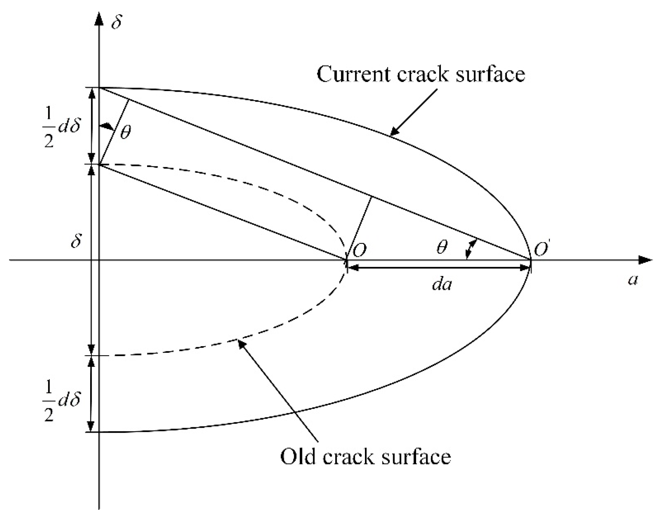
The detailed derivations of the small-timescale model can be found in [29] and a brief introduction of this model is presented here. The basis of this FCG model is the incremental crack growth at any arbitrary small incremental time in a loading cycle. Figure 1 shows the geometric relationship constructed between the instantaneous crack growth kinetics and the crack tip opening displacement (CTOD). Thus, the crack growth rate $da$ is calculated by:

$$da=(ctg\theta /2)d\delta =Cd\delta ,$$

(20)

where $\theta$ is the crack tip opening angle (CTOA), $\delta$ is the CTOD, and $C=ctg\theta /2$. It is assumed that the crack growth in Equation (20) is infinitesimal. The CTOA changes from 90° to a very small angle beyond a certain length until the final failure. Thus, the CTOA is assumed approximately to be a function of material properties and the applied loading, which can be expressed as:

$$\theta =\frac{\pi }{2}-\frac{\pi }{2}\frac{\Delta K-\Delta K_{th}}{K_c-\Delta K_{th}},$$

(21)

where $\Delta K$ is the stress intensity factor range, $\Delta K_{th}$ is the intrinsic threshold stress intensity factor, and $K_c$ is the fracture toughness value. $\Delta K_{th}$ corresponds with the intrinsic material resistance to the FCG. In this study, the FCG problem is a predominantly plane stress problem for surface cracks. Considering the effect of material strain hardening, the CTOD can be expressed as:

$$\delta =\lambda {\sigma }^{2}a,$$

(22)

where $\lambda =\frac{3\pi }{8E{\sigma }_y}$ is a constant of material property, $\sigma$ is the nominal stress, $E$ is Young’s modulus, and ${\sigma }_y$ is the yield stress. According to Figure 1, when the crack tip grows from $O$ to $O^{\prime }$, the increment of CTOD ignoring the high order terms can be expressed as:

$$d\delta ={\delta }^{\prime }-\delta =\lambda {(\sigma +d\sigma )}^2(a+da)-\lambda {\sigma }^{2}a\approx \lambda (2\sigma ad\sigma +{\sigma }^{2}da),$$

(23)

Figure 1. Schematic illustration of crack tip geometry.

Substituting Equation (23) into Equation (20), the instantaneous crack growth rate can be expressed as:

$$\frac{1}{C\lambda a}\frac{da}{dt}=\frac{2\sigma }{1-C\lambda {\sigma }^2}\frac{d\sigma }{dt},$$

(24)

The previous discussion can only be applied when the crack grows. Nevertheless, the crack tip plastic zone is critical for FCG and the reverse plastic zone produces a compressive residual stress after unloading. Due to the energy principle and the reverse plastic zone effect, the crack growth may stop during the initial part of the loading cycle as well as during the unloading cycle. Using the hypotheses for the non-uniform crack growth kinetics, the general expression of the instantaneous crack growth rate under arbitrary loading histories is:

$$\dot{a}=H(\dot{\sigma })·H(\sigma -{\sigma }_{ref})·\frac{2C\lambda }{1-C\lambda {\sigma }^2}·\dot{\sigma }·\sigma ·a,$$

(25)

where $H(x)=\{\begin{array}{cc}1,& \mathrm{if} x>0\\ 0,& \mathrm{if} x\le 0\end{array}$ is the Heaviside function and ${\sigma }_{ref}$ is the reference applied stress level. Crack will only grow beyond a certain stress level ${\sigma }_{ref}$ in the loading path. A detailed calculation of ${\sigma }_{ref}$ on the basis of the interaction of forward and reversed plastic zone can be found in [29].

The relationship between the classical FCG model ($da/dN$ curves) and the presented FCG model is investigated by rewriting the Equation (24). In addition, the crack only grows when $\sigma >{\sigma }_{ref}$ according to the previous discussion. The instantaneous crack growth rate is integrated within a loading cycle can be calculated by direct time integration as:

$${\displaystyle {\int }_{a_0}^{a_0+\Delta a}\frac{da}{C\lambda a}}={\displaystyle {\int }_{{\sigma }_{\min }}^{{\sigma }_{\max }}\frac{2\sigma d\sigma }{1-C\lambda {\sigma }^2}}={\displaystyle {\int }_{{\sigma }_{ref}}^{{\sigma }_{\max }}\frac{2\sigma d\sigma }{1-C\lambda {\sigma }^2}},$$

(26)

Accordingly, the equivalent cycle-based formulation of the small-timescale model can be obtained by solving the integral at both ends of the integral of Equation (24). The length increment $\Delta a$ during one cycle can be expressed as:

$$\Delta a=\frac{da}{dN}=\frac{\pi C\lambda a\left({\sigma }_{\max }{}^2-{\sigma }_{ref}{}^2\right)}{\pi \left(1-C\lambda {\sigma }_{\max }{}^2\right)}=\frac{C\lambda \left(K_{\max }{}^2-K_{ref}{}^2\right)}{\pi \left(1-C\lambda {\sigma }_{\max }{}^2\right)},$$

(27)

where:

$$K_{ref}=\frac{-\left(3{\sigma }_y-2R{\sigma }_{\max }\right)+\sqrt{{\left(3{\sigma }_y-2R{\sigma }_{\max }\right)}^2-4{\sigma }_{\max }\left[R^2{\sigma }_{\max }-\left(2R+1\right){\sigma }_y\right]}}{2}\sqrt{\pi a},$$

(28)

where $R={\sigma }_{\min }/{\sigma }_{\max }$ is the stress ratio. In order to calculate the $K_{ref}$, it is assumed that crack starts to grow when the boundary of the forward plastic zone reaches the boundary of the previous reverse plastic zone. Equation (27) is used to predict the FCG under constant amplitude loading. The predicted FCG rate already includes the stress ratio effects. The presented model shows better accuracy compared with the traditional reversal-based model in previous research. For various time and length scales, the continuous crack length can be calculated by the direct time integration of the general expression of the presented FCG model (Equation (25)). The objective of this study was to adopt the previously discussed small-timescale model for the uncertainty quantification in the FCG analysis. The small-timescale model is fundamentally different from the classical cycle-based FCG and it can easily be utilized on any timescale and over any crack-length range.

3.2. Uncertainty Quantification in FCG

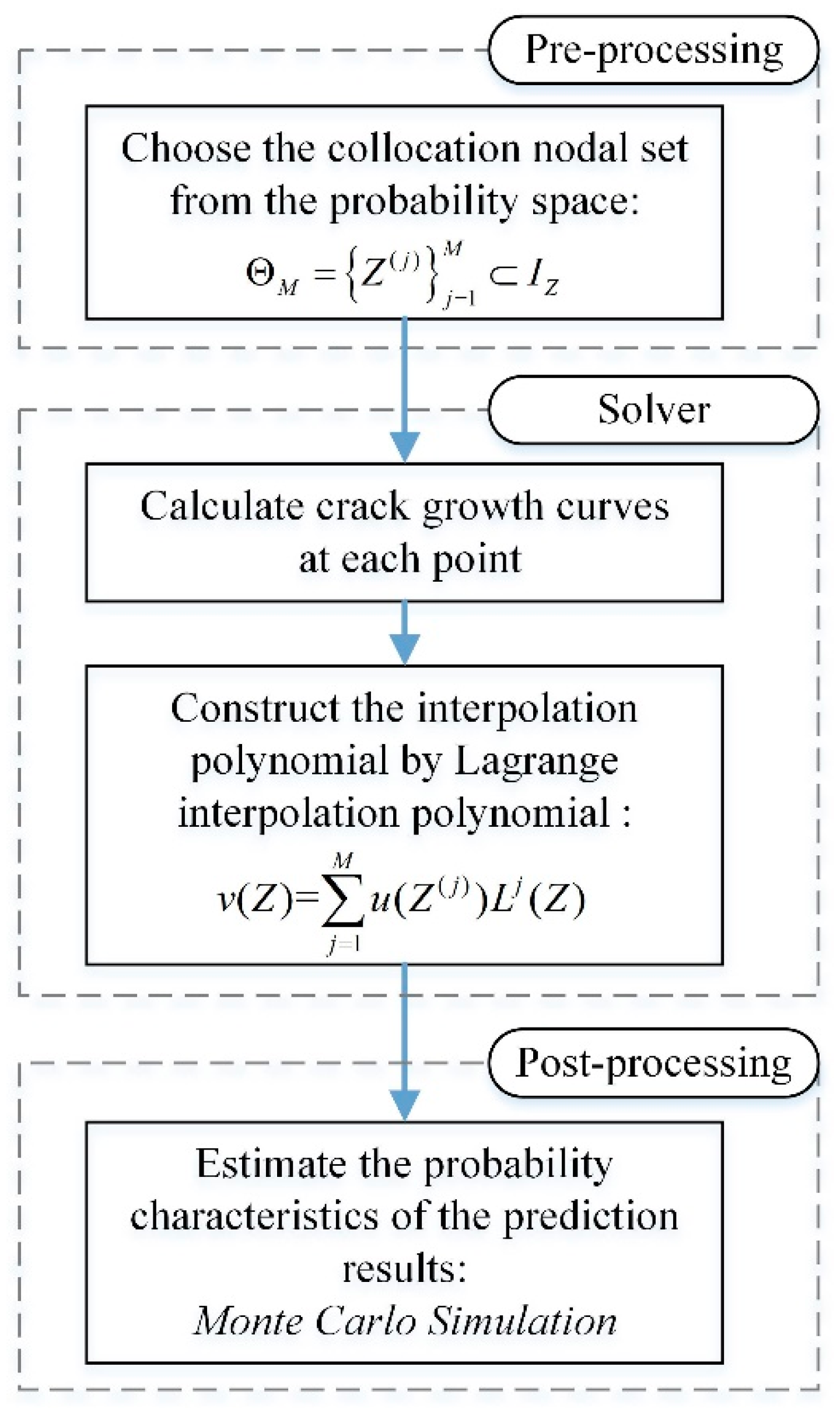
The presented stochastic collocation method is addressed accounting for uncertainty quantification in the small-timescale FCG model. The stochastic collocation separates uncertainty quantification from solving differential equations. The framework of the approach includes four steps. First, define the uncertainty sources and the probability space in the study and choose the nodal set ${\Theta }_M^d$ from the probability space based on the extrema of Chebyshev polynomials and the Smolyak algorithm. Second, solve the deterministic differential equations (Equation (27)) of the small-timescale FCG model at the nodal set. Then, the Lagrange interpolation polynomial is employed to construct the interpolation polynomial for remaining useful life prediction based on the nodal set and the solution set. Finally, estimate the probability characteristics of the prediction results by MC simulation as the post process. The uncertainty quantification framework of the stochastic collocation method is shown in Figure 2.

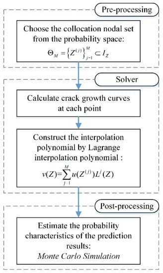
Figure 2. The framework of the proposed approach.

3.3. The Remaining Useful Life Prediction

The remaining useful life prediction is performed at an inspection point when the crack length is estimated as initial crack length $a_0$. The component will end in fatigue failure when the crack propagates from $a_0$ to the critical length $a_c$ in the small-timescale FCG model. According to the previous discussion, the crack growth rate under constant amplitude loading is employed here. Let us rewrite the formulation of crack growth rate:

$$f(a)=\frac{da}{dN}=\frac{C\lambda \left(K_{\max }{}^2-K_{ref}{}^2\right)}{\pi \left(1-C\lambda {\sigma }_{\max }{}^2\right)},$$

(29)

where $N$ is the number of loading cycles when the crack length propagates from $a_0$ to the critical length $a_c$. Then the crack growth process is established by solving the following equation using the Runge-Kutta algorithm:

$$\{\begin{array}{l}da/dN=f(a)\hfill \\ {a|}_{N=0}=a_0\hfill \end{array},$$

(30)

The remaining useful life $N$ at the inspection point can be expressed as:

$$N={\displaystyle {\int }_{a_0}^{a_c}\frac{C\pi (1-C\lambda {\sigma }_{\max }^2)}{\lambda (K_{\max }^2-K_{ref}^2)}}da,$$

(31)

The random input parameters in the fatigue crack propagation can be denoted by $Z=\left(Z_1,\dots ,Z_d\right)$ with $d$ variables. The distributions of the random parameters are assumed to be independent and identical. Then the remaining useful life $N$ is denoted by a function of the random parameters $Z$ as $N(Z)$.

4. Results and Discussion

In order to show the efficiency and accuracy of the proposed method, uncertainty quantification in the crack growth model of a metal plate is implemented with the stochastic collocation method using the experimental data available in previous literature [35]. First, the crack growth curves are established and the uncertainty parameters are defined in the FCG model. Then the stochastic collocation method is applied to predict the remaining useful life accounting for the uncertainty. The prediction results are compared with the experimental data from the literature.

4.1. FCG Analysis of A Metal Plate

The experimental data on 7075-T6 aluminum alloy plate specimens with a center through crack (Figure 3) taken from the above research are collected to investigate the proposed approach of uncertainty quantification for FCG.

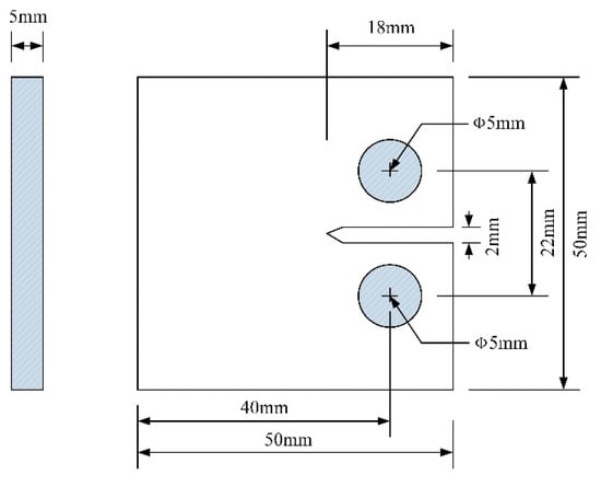
Figure 3. Illustration of the specimen geometry.

The test was conducted under constant amplitude loading (P_max = 2000 N, P_max = 200 N, stress ratio R = 0.1) according to the ASTM standard. Seven sets of 7075-T6 aluminum alloy specimen experiments are published. For easier access to the information in the previous paper, some essential information is presented here: The material and geometry properties of the specimen and the corresponding test data are listed in Table 1 and Table 2, respectively. Figure 4 shows the seven raw data curves under constant amplitude loading. It can be observed that the scatter of raw data curves exists due to the material uncertainty. Based on the test data, the initial crack length is a_c = 0.011 m and the critical length is set as a_c = 0.0258 m to investigate the remaining useful life prediction.

Table 1. Material and geometry properties of plate specimens.

Specimen Material	Ultimate Strength (MPa)	Yield Strength (MPa)	Young’s Modulus (MPa)	Plate Width (mm)	Plate Thickness (mm)
Al 7075-T6	573~582	502~516	71.7	40	5

Table 2. Test data of crack growth length.

Specimen	01	02	03	04	05	06	07
N	a (mm)	a (mm)	a (mm)	a (mm)	a (mm)	a (mm)	a (mm)
0	10.921	10.913	10.921	10.992	10.921	10.921	10.931
1000	11.024	11.216	11.056	11.201	11.102	11.178	11.102
2000	11.153	11.486	11.266	11.452	11.344	11.376	11.353
3000	11.326	11.733	11.476	11.750	11.569	11.580	11.589
4000	11.545	11.993	11.638	12.137	11.734	11.837	11.755
5000	11.778	12.416	11.814	12.521	11.947	12.128	11.946
6000	12.005	12.778	12.020	12.843	12.224	12.400	12.184
7000	12.237	12.939	12.216	13.141	12.478	12.618	12.412
8000	12.491	13.484	12.435	13.541	12.724	12.890	12.671
9000	12.747	13.882	12.698	14.031	12.983	13.200	12.956
10,000	12.967	14.414	12.990	14.497	13.262	13.435	13.216
11,000	13.210	14.797	13.277	15.069	13.598	13.714	13.517
12,000	13.523	15.222	13.536	15.755	14.005	14.040	13.850
13,000	13.904	15.707	13.780	16.443	14.441	14.314	14.132
14,000	14.290	16.214	14.070	17.249	14.762	14.699	14.407
15,000	14.681	16.797	14.413	18.141	15.060	15.260	14.708
16,000	15.145	17.587	14.780	18.953	15.569	15.889	15.033
17,000	15.678	18.561	15.256	19.801	16.094	16.439	15.373
18,000	16.260	19.440	15.820	20.910	16.641	16.960	15.735
19,000	16.878	20.103	16.363	22.602	17.436	17.651	16.130
20,000	17.555	21.790	16.964	25.404	18.335	18.503	16.549
21,000	18.400	22.818	17.600		19.209	19.500	17.033
22,000	19.521	25.601	18.167		20.095	20.627	17.625
23,000	20.714		18.840		21.195	21.723	18.197
24,000	22.124		19.741		22.749	23.361	18.808
25,000	24.323		20.748		24.992	25.890	19.616
26,000			21.374				20.313
27,000			23.258				21.681
28,000			25.682				24.986

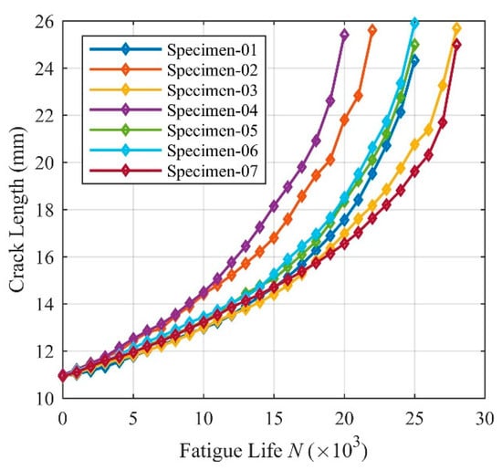
Figure 4. Experimental data under constant amplitude loading.

In this study, it is assumed that the uncertainty comes from the model parameters uncertainty. To generate the simulated crack growth curves, the first step is to quantitate the statistics of the material crack growth parameters. The small-timescale model has four independent underlying parameters to be determined in Equation (27), i.e., the Young’s modulus $E$, the intrinsic threshold stress intensity factor $\Delta K_{th}$, the fracture toughness value $K_c$, and the yield strength ${\sigma }_y$. According to the reference [35], the Young’s modulus $E$ is assumed to be a constant. The randomness in the crack growth is represented by three random variables $\Delta K_{th}$, $K_c$, and ${\sigma }_y$. Then according to the reference [6] and [37], the distribution characteristics of these random variables are determined by fitting crack growth data from the literature. It is found that the lognormal distribution is appropriate for the materials investigated in this paper (as shown in Table 3).

Table 3. Statistical characteristics of model parameters.

Variable	$\mathbf{\Delta }{\mathit{K}}_{\mathit{t}\mathit{h}}(\mathbf{MPa}\times {\mathbf{m}}^{1/2})$	${\mathit{K}}_{\mathit{c}}(\mathbf{MPa}\times {\mathbf{m}}^{1/2})$	${\mathit{\sigma }}_{\mathit{y}}(\mathbf{MPa})$
Mean value	0.8	32	520
Standard deviation	0.011	2.72	30.32

In addition, the stress intensity factor range for the crack tip specimen according to ASTM E647-08 can be calculated by:

$$\Delta K=\frac{\Delta P}{B\sqrt{W}}·\frac{(2+\alpha )}{{(1-\alpha )}^{3/2}}(0.886+4.64\alpha -13.32{\alpha }^2+14.372{\alpha }^3-5.6{\alpha }^4),$$

(32)

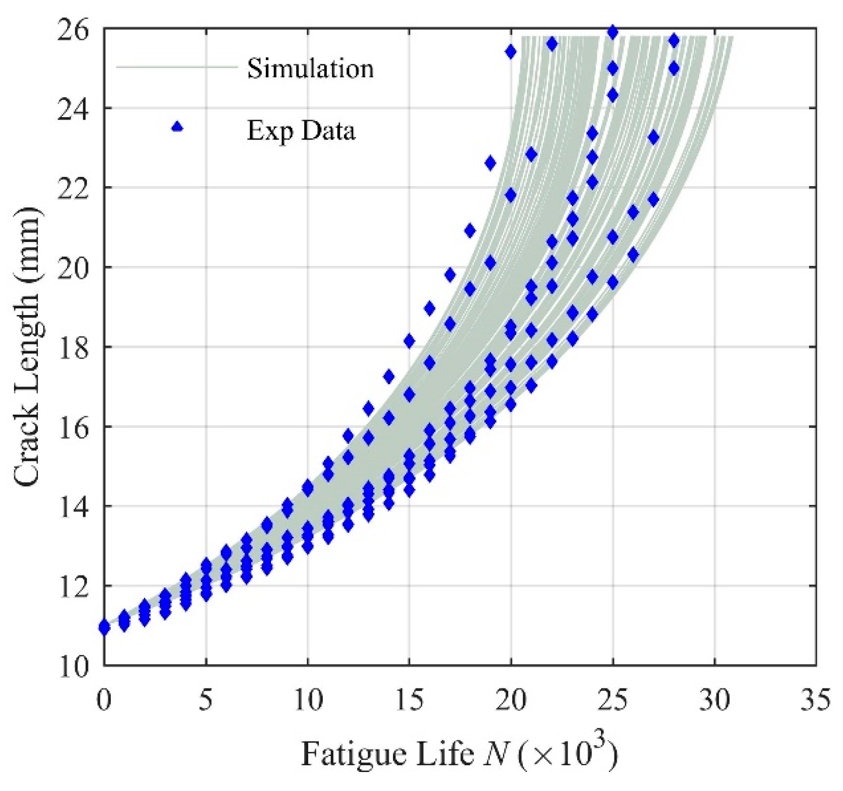
where α = a/W, and the calculation is valid when $\alpha \ge 0.2$. B and W are the thickness and the width of the specimen, respectively. The generated crack growth curves by a directed Monte Carlo simulation (10000 samples) show a general satisfactory agreement compared with the seven raw test data curves (Figure 5), which indicates the ability of the small-timescale model to describe the fatigue propagation.

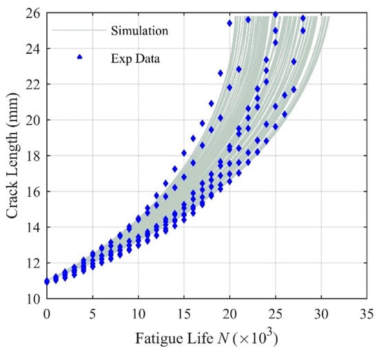
Figure 5. Crack length under constant amplitude loading.

The negligible inconsistency may be caused by different types of uncertainty including natural variability in local geometry, variant loading conditions, and data uncertainty due to measurement errors during experiment, which are over the range of this study. In this investigation, due to the lack of the exact solution of the problem, the prediction results from the proposed method are compared with the results from Monte Carlo simulation, which is considered as the real distribution of the remaining useful life.

4.2. The Stochastic Collocation Method for Remaining Useful Life Prediction

Based on the small-timescale FCG model under constant amplitude loading (Equation (27)), the remaining useful life $N$ of the 7075-T6 aluminum alloy plate can be expressed as Equation (31).

When calculating the remaining useful life in the uncertainty damage prognosis, the material parameters $K_c$, $\Delta K_{th}$ and ${\sigma }_y$ are sampled from the prescribed lognormal distributions. Therefore, the remaining useful life prediction formula for the specimen with uncertainty is:

$$N(Z)={\displaystyle {\int }_{a_0}^{a_c}\frac{C\pi (1-C\lambda {\sigma }_{\max }^2)}{\lambda (K_{\max }^2-K_{ref}^2)}}da, Z\in I_Z,$$

(33)

where $Z=(K_c,\Delta K_{th},{\sigma }_y)$ is the set of independent random variables, and $I_Z$ is the probability space. The quantization interval of the random variable is defined as $\left[\mu -3\sigma ,\mu +3\sigma \right]$ to ensure the probability of the value outside the interval is less than 0.003. Thus, the probability space is set as:

$$I_Z=[0.767,0.833]\times [23.84,40.16]\times [459.04,580.96],$$

(34)

In the stochastic collocation method, the three-dimensional standard probability space ${[-1,1]}^3$ is required by using the linear transformation of the previous probability space.

The core issue for the implementation of the Smolyak sparse grid is the choice of the nodal set depending on the level of interpolation k. To investigate the computational accuracy, the relative cumulative error $er{r}_S$ is defined as:

$$er{r}_S=\frac{{\Vert N_k(z)-N(z)\Vert }_2}{{\Vert N(z)\Vert }_2} z\in I_z,$$

(35)

and the norm is:

$${\Vert N(z)\Vert }_2=\sqrt{{\displaystyle {\int }_{I_z}{\left|N(z)\right|}^{2}dz}},$$

(36)

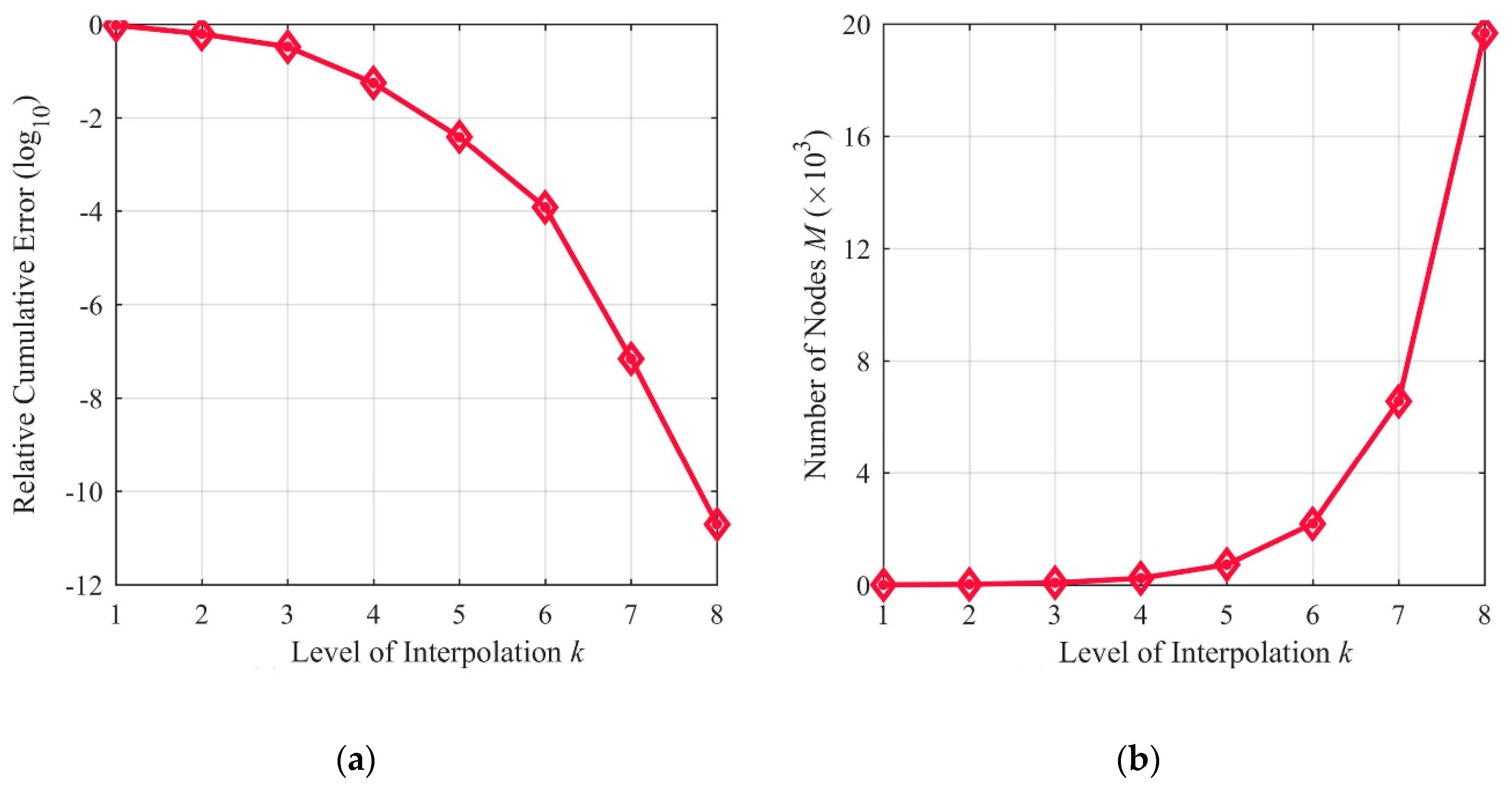
where $N_k(z)$ is the k-level interpolation polynomial. The relative cumulative error decreases rapidly as the level of interpolation increases as shown in Figure 6a. On the other hand, the computational efficiency of the proposed approach is considered by the total number of nodes for the three-dimensional interpolation problem, which is also the number of solving the differential equations $M$ (Figure 6b). According to the above discussion, the level of interpolation $k=5$ is appropriate to balance the computational accuracy and efficiency with $er{r}_S=3.86\times {10}^{-3}$ and $M=727$. Take for example, the elapsed time of directly solving the differential equations (9.1034 s) is more than three times as the elapsed time using $N_5(z)$ (2.7600 s) at 10000 samples. In this study, $N_5(z)$ is selected as the interpolation polynomial of the remaining useful life taking advantage of the efficient sparse grid method.

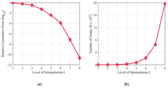
Figure 6. Influence of the level of interpolation: (a) Relative cumulative error; (b) Number of nodes.

4.3. Results of Remaining Useful Life Prediction

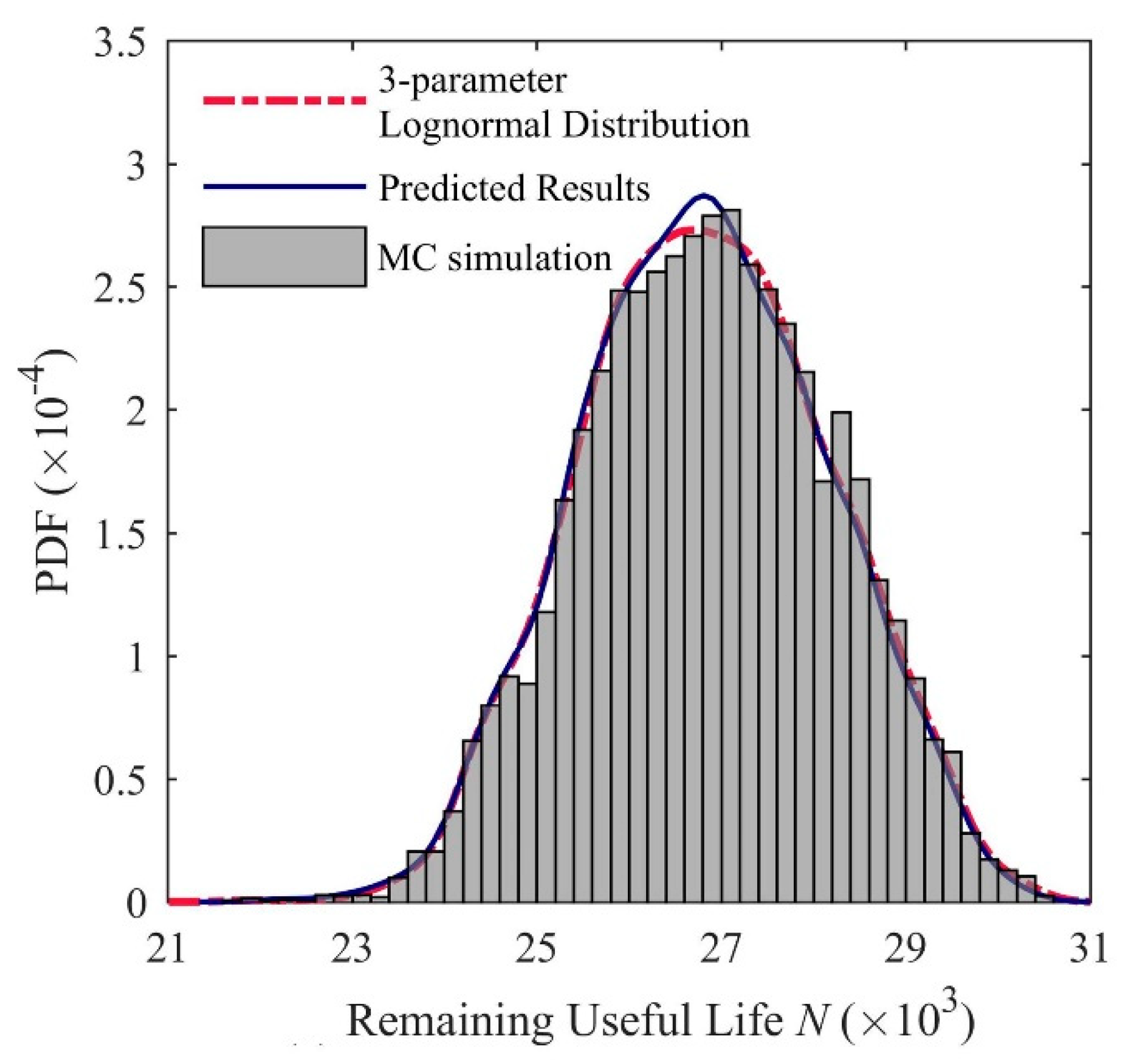
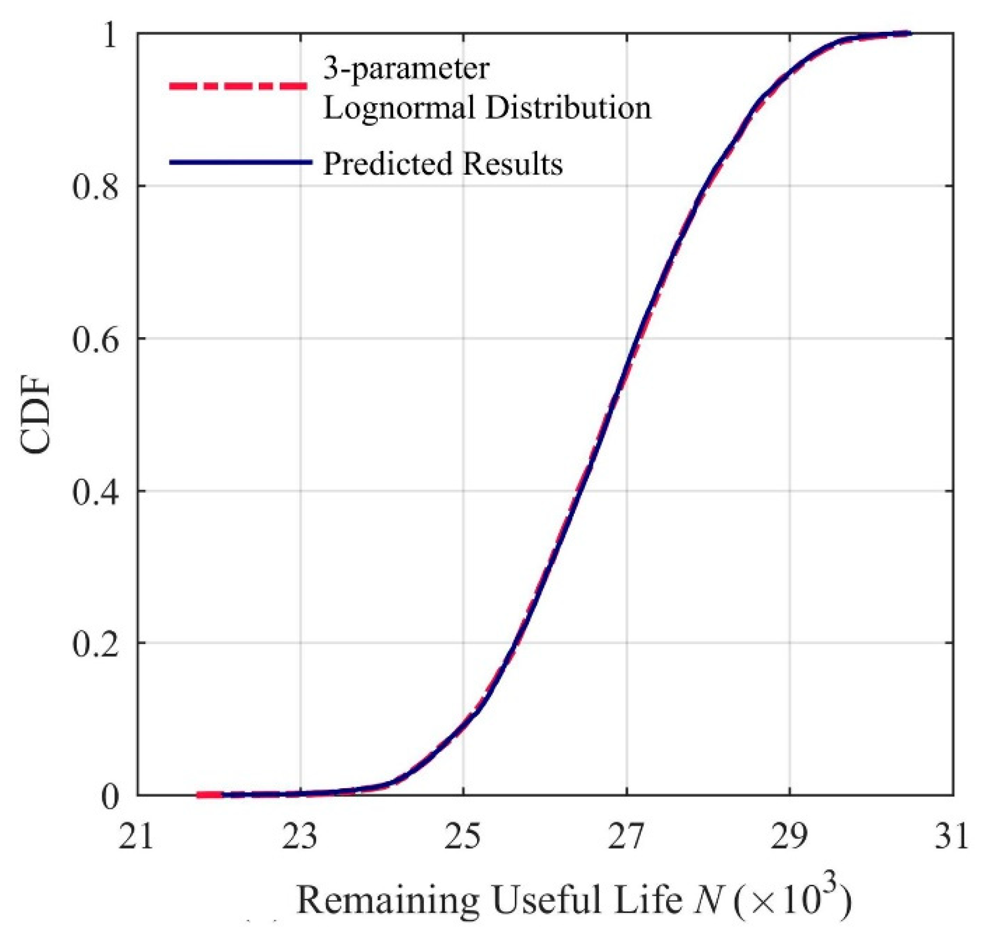
The mean value and the standard deviation of the remaining useful life $N$ are convergent to $[2.68\times {10}^4,2.685\times {10}^4]$ and $[1300,1350]$, respectively, when the number of samples is more than 10,000. Therefore, the probability characteristics of $N$ are investigated based on $n=10000$ Monte Carlo samples with the mean value $\overline{X}=26801$ and the standard deviation $S=1325.4$. Due to the enormous number of samples, four types of distribution including uniform distribution, normal distribution, 2-parameter lognormal distribution and 3-parameter lognormal distribution, are used to fit the distribution of N by a Kolmogorov-Smirnov test (K-S test). The K-S test quantifies a distance $D$ between the cumulative distribution function (CDF) of the samples and the CDF of the reference distribution. It is considered that the samples take the specific distribution when $D<D(n,\alpha )$. The null hypothesis is rejected at level α = 0.05, so that the critical distance is defined as $D(10000,0.05)$. Table 4 lists the results of the K-S test indicating that N takes a 3-parameter lognormal distribution. The probability density function can be expressed as:

$$f(N)=\frac{1}{(N-N_0)\ln 10}·\frac{1}{\sqrt{2\pi }\sigma }{e}^{-\frac{{[\lg (N-N_0)-\mu ]}^2}{2{\sigma }^2}},$$

(37)

where $N_0$, $\mu$ and $\sigma$ are constant parameters. The probability density function (PDF) and the CDF of the samples and the 3-parameter lognormal distribution are shown in Figure 7 and Figure 8, and the MC simulation results from solving the differential equations directly are also included for comparison.

Table 4. The results of the K-S test.

The Type of Distribution	K-S Distance $\mathit{D}$	Critical Distance $\mathit{D}(10000,0.05)$	The Level of Significance
Uniform distribution	0.289	0.0136	0
Normal distribution	0.017	0.0136	0.008
2-parameter lognormal distribution	0.016	0.0136	0.012
3-parameter lognormal distribution	0.007	0.0136	0.689

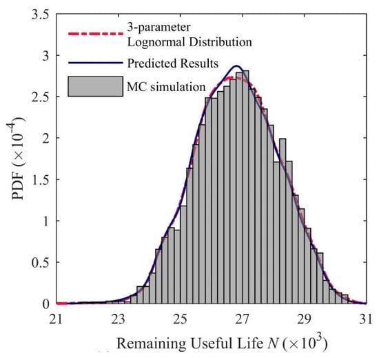
Figure 7. The PDF of remaining useful life.

Figure 8. The CDF of remaining useful life.

Figure 7 and Figure 8 show that the 3-parameter lognormal distribution fit the dataset of the remaining useful life $N$ acceptably, resulting in the following distribution parameters: N₀ = 24306, $\mu =4.408$ and $\sigma =0.0135$. In this study, due to the lack of the experimental data, the results from MC simulation by solving the differential equations in the small-timescale FCG model is considered as the real distribution of the remaining useful life.

It can be observed that the distribution of remaining useful life prediction using the proposed stochastic collocation method shows the goodness of fit of the MC simulation. Furthermore, the predicted remaining useful life with 95% reliability is $N=24610$, which is among the range of experimental results. In addition, it is noted that the total number of nodes, which is also the number of solving the differential equations is 757 and the number of realizations in direct MC simulation is 10000. The present results indicate the proposed approach has the capability to give an overall efficient and accurate prediction of the FCG taking into account uncertainties of input parameters.

5. Conclusions

In this paper, a stochastic collocation approach is developed for uncertainty quantification of remaining useful life prediction in small-timescale FCG model. The presented FCG model improves the accuracy of deterministic prediction of $a-N$ curve based on the instantaneous crack growth increment. Then the stochastic collocation method is utilized to evaluate the remaining useful life prediction uncertainty. The stochastic collocation method based on the gPC expansion is able to reduce the repetitious equation solving significantly. The main conclusions of this research are:

(1)

The FCG curves predicted by the Monte Carlo simulation of the small-timescale model considering the uncertainty parameters agreed well with the experimental data under constant amplitude loading. It can be observed that parameter uncertainties do exist in FCG analysis. Besides, the small-timescale model shows a continuous relationship between the fatigue crack length and the loading history.

(2)

The remaining useful life predictions obtained from the proposed approach were compared with the Monte Carlo simulation results for the plate specimen. The comparisons show that the proposed approach can greatly improve the efficiency and accuracy for uncertainty quantification in FCG analysis by utilizing the stochastic collocation method.

(3)

The significant computation efficiency of this uncertainty quantification approach for FCG can be potentially applied to much more complicated multi-dimensional problems for crack and damage propagations. Moreover, this study focuses on the material uncertainty quantification and other types of uncertainties can be involved in potential applications.

References

- Farrar, C.R.; Lieven, N.A. Damage prognosis: The future of structural health monitoring. Philos. Trans. Math. Phys. Eng. Sci. 2007, 365, 623–632. [Google Scholar] [CrossRef] [PubMed]
- Novak, E.; Ritter, K. High dimensional integration of smooth functions over cubes. Numer. Math. 1996, 75, 79–97. [Google Scholar] [CrossRef]
- Jallouf, S.; Casavola, K.; Pappalettere, C.; Pluvinage, G. Assessment of undercut defect in a laser welded plate made of Ti–6Al–4V titanium alloy with probabilistic domain failure assessment diagram. Eng. Fail. Anal. 2016, 59, 17–27. [Google Scholar] [CrossRef]
- Long, X.Y.; Liu, K.; Jiang, C.; Xiao, Y.; Wu, S.C. Uncertainty propagation method for probabilistic fatigue crack growth life prediction. Theor. Appl. Fract. Mech. 2019, 103, 102–268. [Google Scholar] [CrossRef]
- Lin, Y.; Ding, Z.; Zio, E. Fatigue crack growth assessment method subject to model uncertainty. Eng. Fract. Mech. 2019, 219, 106–624. [Google Scholar] [CrossRef]
- Liu, Y.; Mahadevan, S. Probabilistic fatigue life prediction using an equivalent initial flaw size distribution. Int. J. Fatigue 2009, 31, 476–487. [Google Scholar] [CrossRef]
- Chen, M.; Fang, W.; Yang, C.; Xie, L. Bayesian prediction and probabilistic model of fatigue cracks in steel structures. Eng. Fail. Anal. 2019, 103, 335–346. [Google Scholar] [CrossRef]
- Shiao, M.; Chen, T.; Mao, Z. Probabilistic Maintenance-Free Operating Period via Bayesian Filter with Markov Chain Monte Carlo (MCMC) Simulations and Subset Simulation. In Model Validation and Uncertainty Quantification; Springer: Cham, Switzerland, 2019; Volume 3, pp. 225–234. [Google Scholar]
- Bäck, J.; Nobile, F.; Tamellini, L.; Tempone, R. Stochastic Spectral Galerkin and Collocation Methods for PDEs with Random Coefficients: A Numerical Comparison; Springer: Berlin, Heidelberg, Germany, 2011; pp. 43–62. [Google Scholar]
- Xiu, D.; Hesthaven, J.S. High-order collocation methods for differential equations with random inputs. Siam. J. Sci. Comput. 2005, 27, 1118–1139. [Google Scholar] [CrossRef]
- Najm, H.N. Uncertainty quantification and polynomial chaos techniques in computational fluid dynamics. Annu. Rev. Fluid Mech. 2009, 41, 35–52. [Google Scholar] [CrossRef]
- Reagan, M.T.; Najm, H.N.; Debusschere, B.J.; Le Maître, O.P.; Knio, O.M.; Ghanem, R.G. Spectral stochastic uncertainty quantification in chemical systems. Combust. Theor. Model. 2004, 8, 607–632. [Google Scholar] [CrossRef]
- Li, H.; Zhang, D. Probabilistic collocation method for flow in porous media: Comparisons with other stochastic methods. Water Resour. Res. 2007, 43, W09409. [Google Scholar] [CrossRef]
- Foo, J.; Yosibash, Z.; Karniadakis, G.E. Stochastic simulation of riser-sections with uncertain measured pressure loads and/or uncertain material properties. Comput. Method Appl. Mech. 2007, 196, 4250–4271. [Google Scholar] [CrossRef]
- He, J.; Gao, S.; Gong, J. A sparse grid stochastic collocation method for structural reliability analysis. Struct. Saf. 2014, 51, 29–34. [Google Scholar] [CrossRef]
- Riahi, H.; Bressolette, P.; Chateauneuf, A. Random fatigue crack growth in mixed mode by stochastic collocation method. Eng. Fract. Mech. 2010, 77, 3292–3309. [Google Scholar] [CrossRef]
- Zhao, F.; Tian, Z.; Zeng, Y. A stochastic collocation approach for efficient integrated gear health prognosis. Mech. Syst. Signal Process. 2013, 39, 372–387. [Google Scholar] [CrossRef]
- Beck, A.T.; Gomes, W.J.D.S. Stochastic fracture mechanics using polynomial chaos. Probabilistic Eng. Mech. 2013, 34, 26–39. [Google Scholar] [CrossRef]
- Sankararaman, S.; Ling, Y.; Mahadevan, S. Uncertainty quantification and model validation of fatigue crack growth prediction. Eng. Fract. Mech. 2011, 78, 1487–1504. [Google Scholar] [CrossRef]
- Tang, H.; Li, D.; Li, J.; Xue, S. Epistemic uncertainty quantification in metal fatigue crack growth analysis using evidence theory. Int. J. Fatigue 2017, 99, 163–174. [Google Scholar] [CrossRef]
- Long, X.Y.; Jiang, C.; Liu, K.; Han, X.; Gao, W.; Li, B.C. An interval analysis method for fatigue crack growth life prediction with uncertainty. Comput. Struct. 2018, 210, 1–11. [Google Scholar] [CrossRef]
- Paris, P.; Erdogan, F. A critical analysis crack propagation laws. J. Basic Eng. 1963, 85, 528–534. [Google Scholar] [CrossRef]
- Forman, R.G.; Kearney, V.E.; Engle, R.M. Numerical analysis of crack propagation in cyclic-loaded structures. J. Basic Eng. 1967, 89, 459–463. [Google Scholar] [CrossRef]
- Wolf, E. Fatigue crack closure under cyclic tension. Eng. Fract. Mech. 1970, 2, 37–45. [Google Scholar] [CrossRef]
- Chang, T.; Li, G.; Hou, J. Effects of applied stress level on plastic zone size and opening stress ratio of a fatigue crack. Int. J. Fatigue 2005, 27, 519–526. [Google Scholar] [CrossRef]
- Newman, J.C. A crack opening stress equation for fatigue crack growth. Int. J. Fract. 1984, 24, R131–R135. [Google Scholar] [CrossRef]
- Vasudevan, A.K.; Sadananda, K.; Louat, N. Reconsideration of fatigue crack closure. Scr. Metall. Mater. 1992, 27, 1673–1678. [Google Scholar] [CrossRef]
- Zhang, J.Z.; He, X.D.; Tang, H.; Du, S.Y. Direct high resolution in situ SEM observations of small fatigue crack opening profiles in the ultra-fine grain aluminium alloy. Mater. Sci. Eng. 2008, 485, 115–118. [Google Scholar] [CrossRef]
- Lu, Z.; Liu, Y. Small time scale fatigue crack growth analysis. Int. J. Fatigue 2010, 32, 1306–1321. [Google Scholar] [CrossRef]
- Lu, Z.; Liu, Y. Concurrent fatigue crack growth simulation using extended finite element method. Front. Archit. Civ. Eng. China 2010, 4, 339–347. [Google Scholar] [CrossRef]
- Lu, Z.; Liu, Y. A comparative study between a small time scale model and the two driving force model for fatigue analysis. Int. J. Fatigue 2012, 42, 57–70. [Google Scholar] [CrossRef]
- Wang, H.; Zhang, W.; Zhang, J.; Dai, W.; Zhao, Y. Investigative method for fatigue crack propagation based on a small time scale. Materials 2018, 11, 774. [Google Scholar] [CrossRef]
- Huo, J.; Zhu, D.; Hou, N.; Sun, W.; Dong, J. Application of a small-timescale fatigue, crack-growth model to the plane stress/strain transition in predicting the lifetime of a tunnel-boring-machine cutter head. Eng. Fail. Anal. 2017, 71, 11–30. [Google Scholar] [CrossRef]
- Ye, H.; Wang, T.; Wu, C.; Duan, Z.; Liu, C. A comparative analysis of driving force models for fatigue crack propagation of CFRP-reinforced steel structure. Int. J. Fatigue 2020, 130, 105266. [Google Scholar] [CrossRef]
- Lu, Z.; Liu, Y. Experimental investigation of random loading sequence effect on fatigue crack growth. Mater. Des. 2011, 32, 4773–4785. [Google Scholar] [CrossRef]
- Barthelmann, V.; Novak, E.; Ritter, K. High dimensional polynomial interpolation on sparse grids. ADV Comput. Math. 2000, 12, 273–288. [Google Scholar] [CrossRef]
- Wang, Q.Y.; Kawagoishi, N.; Chen, Q. Fatigue and fracture behaviour of structural Al-alloys up to very long life regimes. Int. J. Fatigue 2006, 28, 1572–1576. [Google Scholar] [CrossRef]
© 2020 by the authors. Licensee MDPI, Basel, Switzerland. This article is an open access article distributed under the terms and conditions of the Creative Commons Attribution (CC BY) license (http://creativecommons.org/licenses/by/4.0/).