Identification of the Flow Properties of a 0.54% Carbon Steel during Continuous Cooling

Abstract

The determinination of material properties is an essential step in the simulation of manufacturing processes. For hot deformation processes, consistently assessed Carreau fluid constitutive model derived in prior works by Schmicker et al. might be used, in which the flow stress is described as a function of the current temperature and the current strain rate. The following paper aims to extend the prior mentioned model by making a distinction, whether the material is being heated or cooled, enhancing the model capabilities to predict deformations within the cooling process. The experimental identifaction of the material parameters is demonstrated for a structural carbon steel with 0.54% carbon content. An approach to derive the flow properties during cooling from the same samples used at heating is presented, which massively reduces the experimental effort in future applications.

1. Introduction

The input of manufacturing process simulations has to include information about the actual process as well as the geometries and the materials being processed. Geometry and process information tend to be easier to obtain, because those are constantly monitored for quality assurance, for instance. The assessment of the material information on the other hand is more challenging, because several factors have to be considered.

A manufacturing process involving a broad range of temperatures and strain rates is rotary friction welding (RFW). In this process, the energy to form a permanent bond is directly introduced in the joining zone in form of frictional heat, which is generated by pressing the parts together while a relative motion is performed. Therefore, through this process temperatures close to the liquidus temperature of the softer material are achieved [1,2] and the strain rates reach one-digit values [3,4]. To simulate RFW processes, Schmicker et al. [4,5,6,7] elaborated a non-linear fluid model to describe the material flow. Although there are material models more capable in representing the dependencies of the yield stress on the deformation temperature, the strain rate, the degree of deformation, the phase composition and more, this model is suitable for RFW and for other hot deformation processes, too. A major advantage are the fairly expedient material parameters that can be gathered with only a few samples in a tensile testing routine, in which the test specimen is continuously heated. Besides conducting own experiments, the model can also be parametrized using data from encyclopedias such as [8,9], which significantly lowers the necessary efforts for the application of the process simulation.

As Schmicker et al. define the flow stress solely by steady-state values, the material point history is not taken into account. Similarly, aforementioned encyclopedias may also contain only the first three factors listed previously.

During heating, the microstructure of carbon steels starts to change to austenite by diffusion processes, if the temperature is greater than $A{c}_1$ and which finish at $A{c}_3$. Both, $A{c}_1$ and $A{c}_3$, depend on the rate of heating, which is documented in time-temperature-austenitization (TTA) diagrams as found in [10]. During cooling, the reverse transformation deviates from this and primarly depends on the cooling rate, which is documented in continuous cooling transformation (CCT) diagrams as depicted in Figure 1. Further information in the CCT include the microstructural composition as well as the hardness H, typically in Vickers hardness (HV),which occur at different cooling paths.

The microstructural changes have an impact on the flow properties of the material and the properties during cooling therefore differ from the properties during heating [11]. This should be taken into account in the process simulation if the material is still being deformed during cooling and independently of this in the residual stresses analysis as the yield strength limits the stress formation.

The current paper aims to quantify the flow properties of a 0.54% carbon steel during continuous cooling and to link the gathered results to the properties at heating, which are assumed to match the steady-state reference values, because the investigated temperature range is limited around and below $A{c}_1$ temperature, at which the diffusional transformations just start.

To experimentally determine the material properties, a prior developed testing routine by Schmicker is extended by tests with continuous cooling. Since there exist an infinite number of cooling rates, a practical approach is proposed, which involves the hardnesses and transformation temperatures found in CCT diagrams as shown in Figure 1. This approach based on reference flow properties and hardness values aims to ensure that all model parameters can also be determined using the data available in literature collections. Concerning hot forming processes, data found in deformation CCT diagrams [13] indicate that compared to the cooling rate, the effect of deformations on the hardness is significantly smaller.

2. Materials and Methods

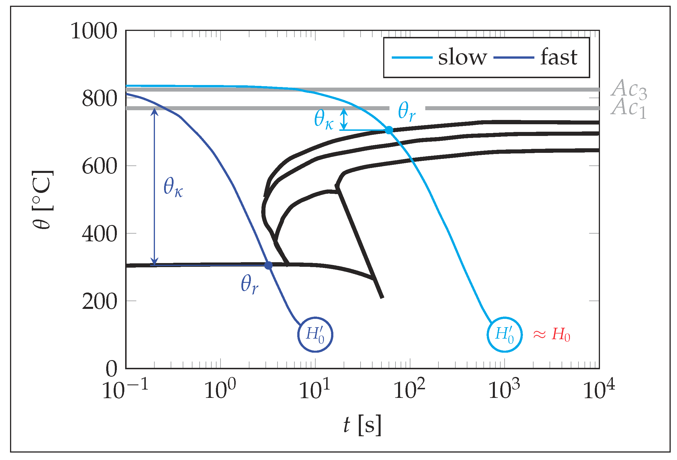
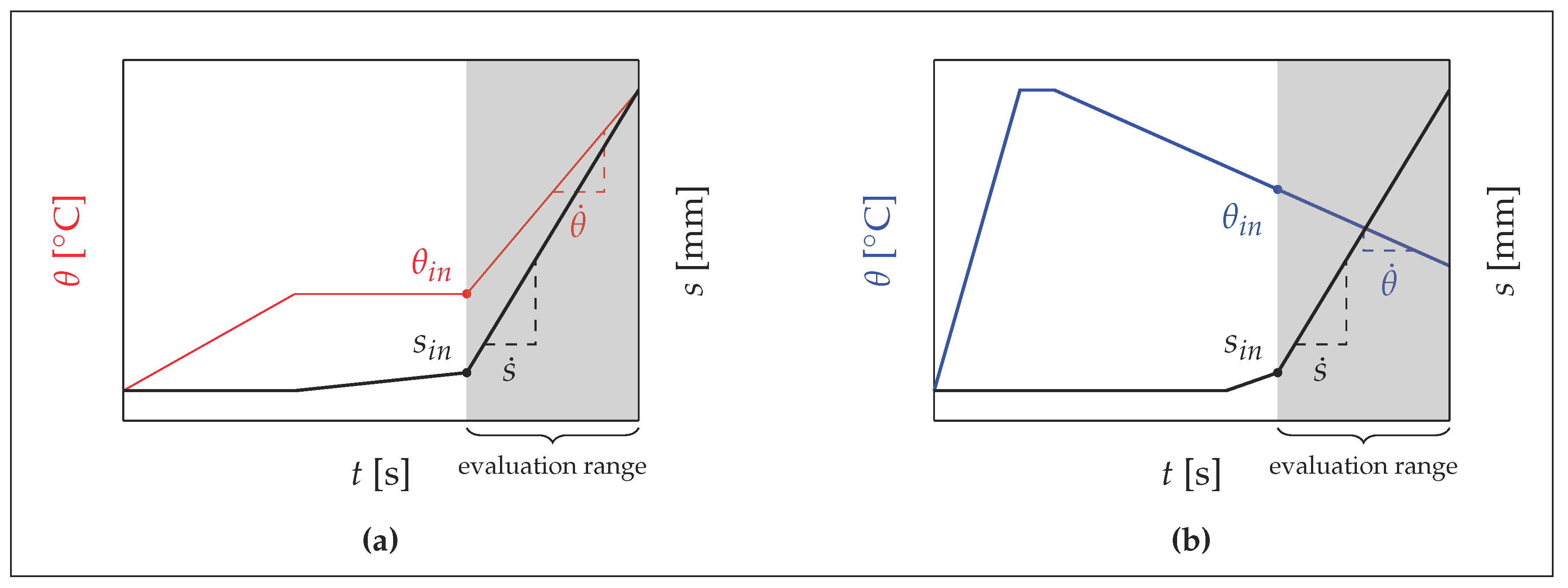
2.1. Mathematical Approach

The description and evaluation of the plastic material properties presented below is based on the following assumptions:

• The material behaves isotropic regarding all mechanical properties.
• Strain hardening effects are negligible compared to the phase transformation effects.
• Compared to the plastic deformations, the elastic, thermal and transformation strains are negligible small.

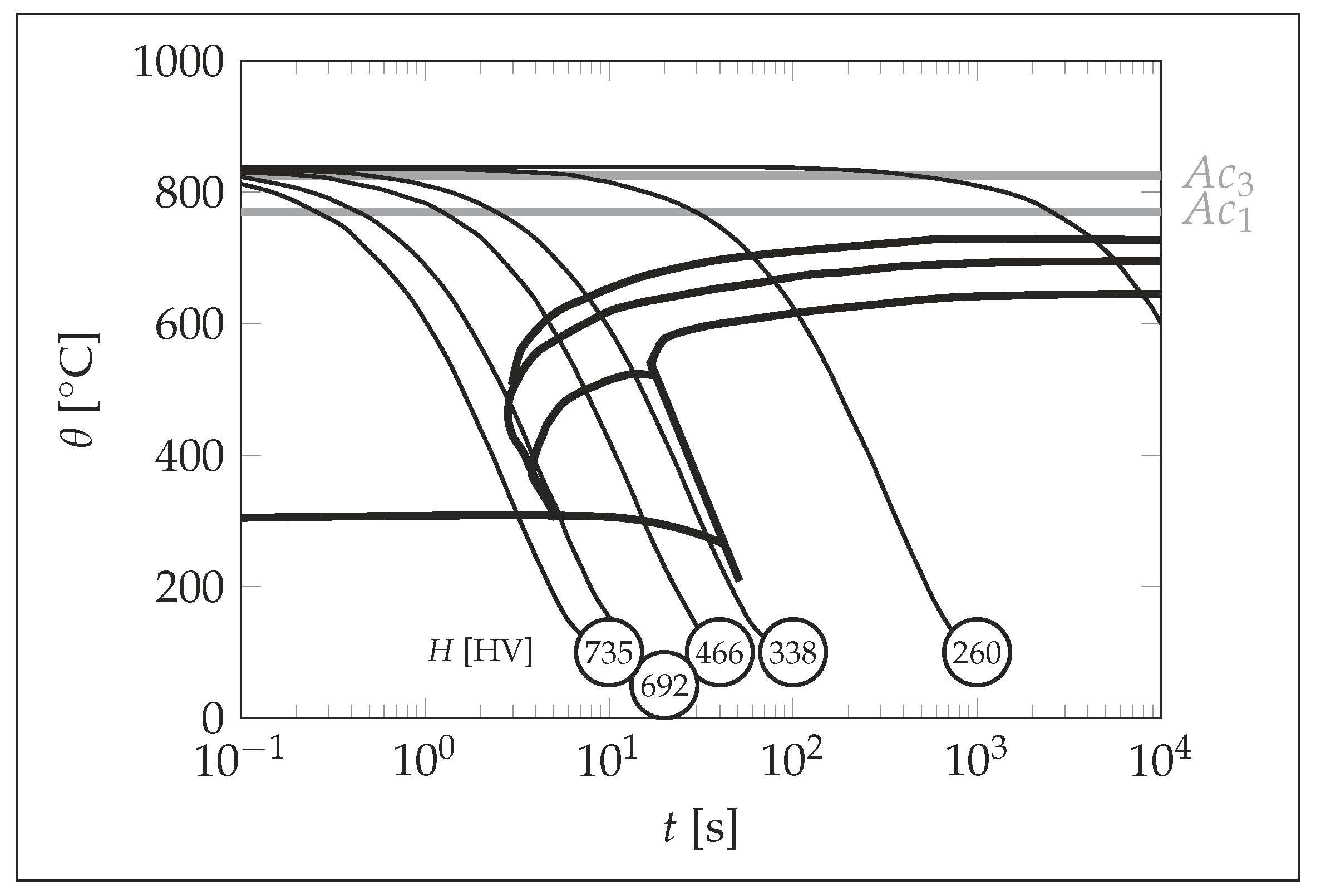
In the Norton–Bailey constitutive model [14], in the double logarithmic depiction the stress–strain rate relation is linear, which can be formulated as

$$\dot{\epsilon }=A{\sigma }^n$$

(1)

or as

$$\frac{\dot{\epsilon }}{{\dot{\epsilon }}_0}={\left(\frac{\sigma }{{\sigma }_0}\right)}^n$$

(2)

in which ${\sigma }_0\left(\theta \right)$ and $n\left(\theta \right)$ are material parameters specified for a reference strain rate ${\dot{\epsilon }}_0$ and as a function of temperature $\theta$. Equation (2) is valid for a wide range of strain rates and materials and documented in several data collections [8,9]. Under the premise that all isothermal flow curves ${\sigma }_{iso}({\theta }_{iso},\dot{\epsilon })$ intersect in one characteristic point $C({\sigma }_C,{\epsilon }_C)$, Schmicker et al. [7] bypass the determination of $n\left(\theta \right)$ for every temperature. Therefore, knowing the point C, the Norton–Bailey exponent can be expressed as

$$n=\frac{log\left(\frac{{\dot{\epsilon }}_C}{{\dot{\epsilon }}_0}\right)}{log\left(\frac{{\sigma }_C}{{\sigma }_0}\right)}$$

(3)

as a feature in the so-called consistently assessed Carreau fluid model. The strain rate sensitivity typically increases with increasing temperatures and to produce higher strain rates, higher stresses are required, which is ensured by

$$\begin{array}{c}\hfill \begin{array}{cc}\hfill {\sigma }_C& >max\left({\sigma }_0(\theta ,{\dot{\epsilon }}_0)\right)\hfill \\ \hfill {\dot{\epsilon }}_C& >{\dot{\epsilon }}_0\hfill \end{array}\end{array}$$

(4)

To distinguish heating and cooling, the flow properties during continuous cooling are subsequently denoted by an apostrophe. Two effects are taken into account for.

Firstly, a heat treatment effect, in which the material either hardens or softens due to microstructural changes. Rapid quenching causes the formation of martensite, which achieves more than twice the hardnesses than ferrite and pearlite. In annealing processes on the other hand, the cooling is typically slow to avoid this transformation.

Secondly, a transformation inertness that causes the transformation to shift to other temperature ranges depending on the cooling rate. The quicker the cooling process, the less is the time for the carbon diffusion processes. If the diffusion can not take place at all, the carbon become trapped in a body-centered tetragonal lattice configuration below martensite start temperature. In Figure 1 it is also seen that even for very slow cooling, the transformation starts well below $A{c}_3$.

Assuming that ${\sigma }_0^{\prime }$ during cooling is not necessarily identical to ${\sigma }_0$ at heating, but similarly shaped, the two curves are linked by adding offset parameters $\kappa$ and ${\theta }_{\kappa }$

$${\sigma }_0^{\prime }(\theta ,\dot{\theta })=\kappa {\sigma }_0(\theta +{\theta }_{\kappa })$$

(5)

for prior discussed transformation effects, depending on $\theta ,\dot{\theta }$.

The hardening factor $\kappa$ can be interpreted as a vertical scaling of ${\sigma }_0\left(\theta \right)$ to account for the heat treating effect as prior applied by Rößler et al. [15]. For its evaluation the linear relation in-between the yield strength ${\sigma }_y$ and the Vickers hardness H [16,17]

$${\sigma }_y=aH+b$$

(6)

is utilized, in which it is physically reasonable that b is zero. It should be mentioned that for other hardness scales the correlation can be non-linear. At room temperature, $\kappa$ can be expressed as the proportion

$$\kappa ({\theta }_0,\dot{\theta })=\frac{{\sigma }_0^{\prime }({\theta }_0,\dot{\theta })}{{\sigma }_0({\theta }_0+{\theta }_{\kappa })}=\frac{H_0^{\prime }\left(\dot{\theta }\right)}{H_0}$$

(7)

in which $H_0$ is the initial hardness corresponding to ${\sigma }_0\left({\theta }_0\right)$ and $H_0^{\prime }$ the hardness after cooling with a specific rate. To couple the hardening to the actual transformation, sigmoid function

$$\kappa (\theta ,\dot{\theta })=\kappa ({\theta }_0,\dot{\theta })-\frac{\kappa ({\theta }_0,\dot{\theta })-1}{2}tanh\left(\frac{2}{{\theta }_r\left(\dot{\theta }\right)-A{c}_1}(\theta -A{c}_1)\right)$$

(8)

limits hardening to the lower temperature range. The parameters $H_0^{\prime }$ and ${\theta }_r$ are either found in the CCT diagram (Figure 2) or can be experimentally determined by indentation and dilatometric testing. The use of the $A{c}_1$ temperature is a recommendation for a free value of this equation, because it guarantees $(\theta \left(\dot{\theta }\right)-A{c}_1)<0$, which must always be fulfilled for mathematical reasons.

To shift ${\sigma }_0\left(\theta \right)$ horizontally due to a transformation inertness, the delay temperature

$${\theta }_{\kappa }(\theta ,\dot{\theta })=\frac{A{c}_1-{\theta }_r\left(\dot{\theta }\right)}{2}tanh\left(\frac{2}{{\theta }_r\left(\dot{\theta }\right)-A{c}_1}(\theta -A{c}_1)\right)$$

(9)

is similar defined as $\kappa$. It is worth mentioning that $\kappa$ and ${\theta }_{\kappa }$ actually start to raise above ${\theta }_r$ to compensate discontinuities of ${\sigma }_0^{\prime }$ introduced by large ${\theta }_{\kappa }$ for martensitic transformations, for instance.

Concerning Equation (3), the characteristic intersection point $C^{\prime }$ has to be re-evaluated, too, to satisfy (4) for $\kappa \gg 1$. To maintain the same high strain rate senstivity at high temperatures around the melting point ${\theta }_M$ and assuming that the low sensitivity for low temperatures will not change, point $C^{\prime }$ is identified using

$$\begin{array}{c}\hfill \begin{array}{cc}\hfill n^{\prime }\left({\theta }_M\right)& =n\left({\theta }_M\right)\hfill \\ \hfill n^{\prime }\left({\theta }_0\right)& =n\left({\theta }_0\right)\hfill \end{array}\end{array}$$

(10)

To estimate hardnesses not documented in the CCT diagram, law of mixture

$$H=\sum _i{\xi }_i{H}_i$$

(11)

as presented by Ion et al. [18] can be applied, in which $\xi$ are the phase fractions of ferrite, pearlite, bainite, martensite, and austenite. The calculation of the phase fraction might be done numerically using evolution equation

$$\dot{\xi }\left(t\right)=\frac{{\xi }_{\infty }\left(\theta \right)-\xi \left(t\right)}{\tau \left(\theta \right)}$$

(12)

by Leblond and Devaux [19].

2.2. Materials

A detailed summary of the chemical composition of the investigated steel is provided in

Table 1. Chemical composition of the investigated 0.54% carbon steel.

C	Si	Mn	P	S
0.54	0.21	0.63	0.008	0.006

. The round tensile specimens used in tensile testing are machined from rods measuring 10 mm in diameter.

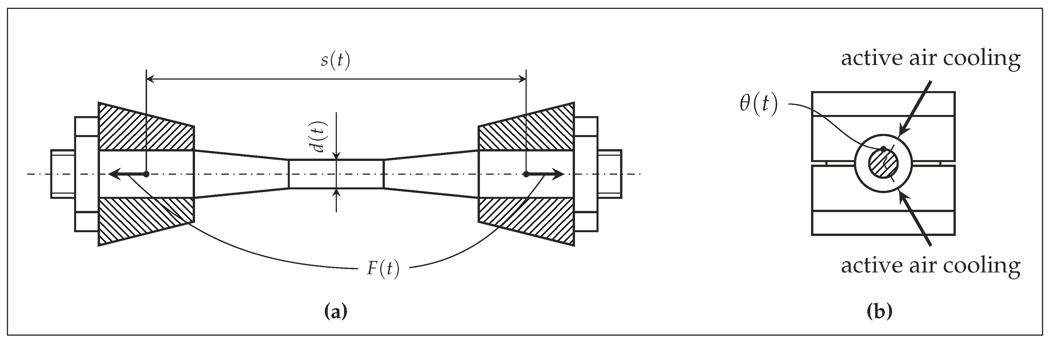
2.3. Experimental Setup

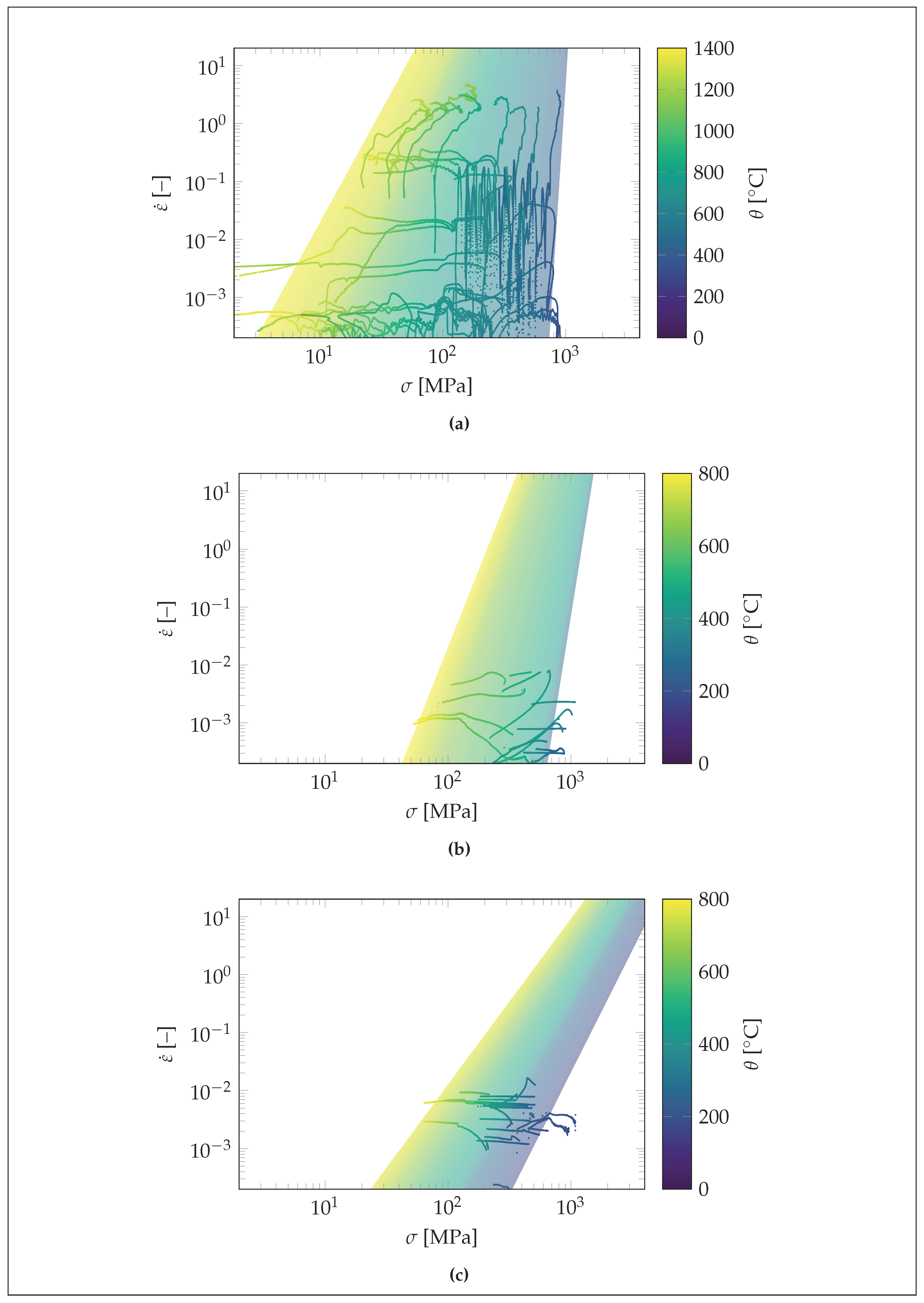
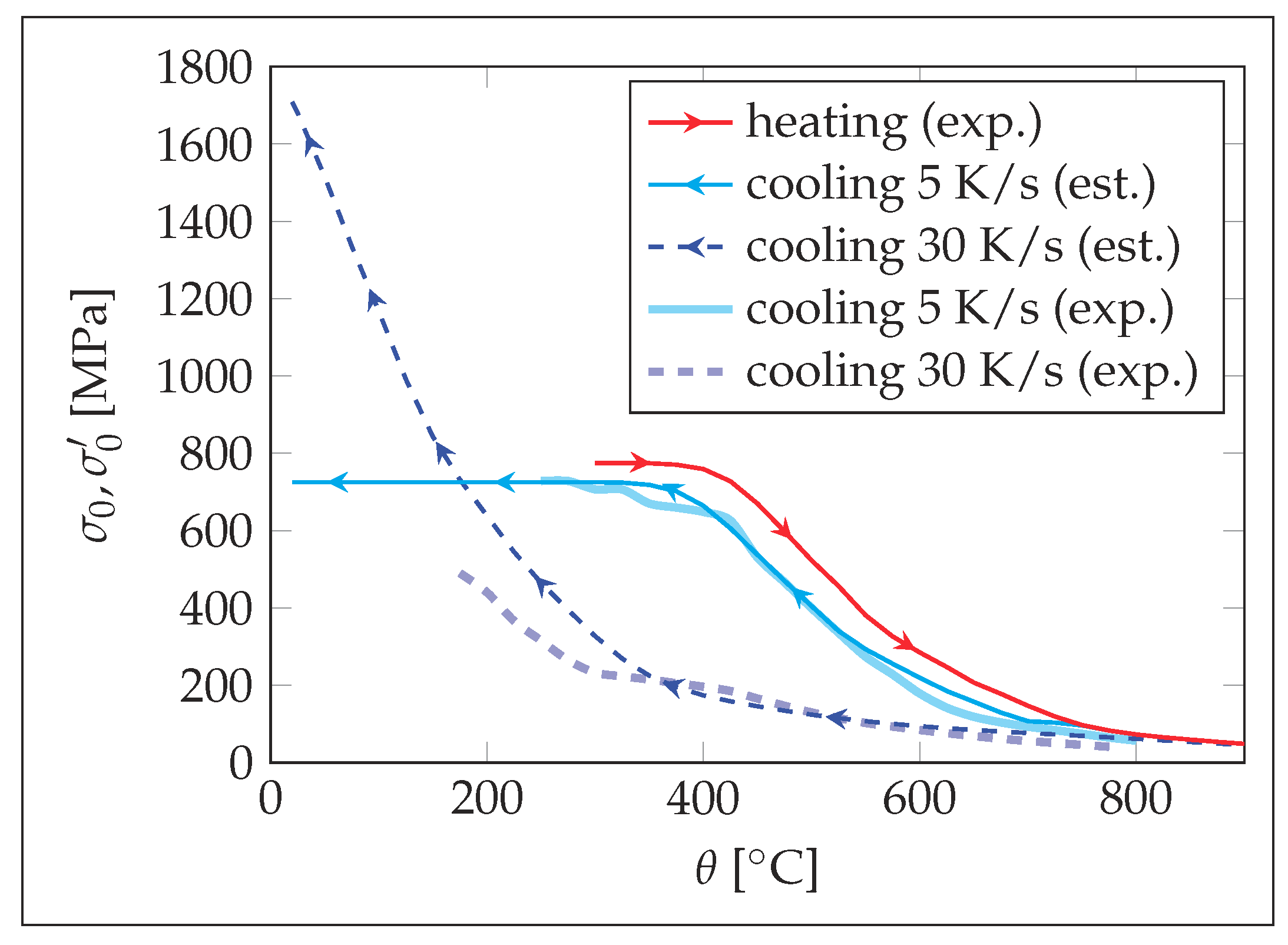
The uniaxial tensile tests were carried out using Gleeble 3500 testing machine at Otto von Guericke University Magdeburg. Part of its capabilities was the execution of displacement controlled, uniaxial tensile tests, while the temperature of the test specimen could be varied using conductive heating at the same time. Figure 3 provides an overview of the setup. Within the machine, the force $F\left(t\right)$ required to produce the stroke $s\left(t\right)$ was captured and an additionally installed extensometer monitored the diameter $d\left(t\right)$ in the axial center of the test specimen. At the same location, the temperature $\theta \left(t\right)$ was measured by welded-on K-type thermo couples, which were used to control the amperage for the conductive heating. The initial diameter in the monitored section was 6 mm based on the permissible force of the testing machine. For cooling upto 30 K/s, two air cooling jets were installed, which aimed at the center of the test specimen. The rate of 30 K/s could be maintained down to 250 ${}^{\circ }\mathrm{C}$, which was well below the martensite start temperature.

In both routines, the specimens were exposed to linear temperature and displacement profiles in the evaluation range (Figure 4). This allowed us to gather information about the flow properties for a number of temperatures in a single test. In order to examine different ranges of $\theta$ and $\dot{\epsilon }$, the start temperature ${\theta }_{in}$ was varied as well as the stroke rate $\dot{s}$. A drawback of altering these parameters simultaneously was that factors such as crystal recovery, recrystallization, and grain growth remained inseparable from the thermal dependence and were therefore averaged in the evaluation of the tensile tests. To overcome elastic deformations, pre-stroke $s_{in}$ was set to 0.3 mm, before the actual evaluation range begins. A comparitive summary of the test conditions during heating and cooling is provided in

Table 2. Summary of test conditions.

	Heating	Cooling
${\theta }_{in}$	≥300 ${}^{\circ }\mathrm{C}$	≤800 ${}^{\circ }\mathrm{C}$
$\dot{\theta }$	1–2000 K/s	5 K/s, 30 K/s
$s_{in}$	0.3 mm
$\dot{s}$	0.003–30 mm/s	0.03–0.3 mm/s

.

In the cooling tests, all test specimens were heated up to 1200 ${}^{\circ }\mathrm{C}$ to trigger the phase transformation to austenite. The controlled cooling process was then started by turning on the air jets, where the central thermocouple was used to ensure constant cooling rates. The cooling rates $\dot{\theta }$ were exemplarly set to 5 K/s, at which it was assumed that the microstructure was similar to the initial one, and to 30 K/s, at which martensite is formed. For heating, test data for about 40 specimens were available by Jüttner and Körner [20] and additional 20 tests were performed for both examined $\dot{\theta }$, because of the narrowed temperature evaluation range.

To evaluate Equation (7), Vickers hardness measurements were carried out across the center of the lateral cross-sections of test specimens, tested with the same cooling routine without applying any axial forces. The indentation locations were arranged in three lines, each of which got 10 points spaced over the diameter, with 2 mm axial spacing.

3. Results

Based on the measured data for $F\left(t\right)$ and $d\left(t\right)$, the longitudinal true stress

$$\sigma =\frac{4F}{\pi d^2}$$

(13)

and the longitudinal true strain rate

$$\dot{\epsilon }=-2\frac{\dot{d}}{d}$$

(14)

were derived.

In order to fit the model according to Equation (3), the generated $\sigma$-$\dot{\epsilon }$-$\theta$ triples were classified by $\theta$ and least squares method was applied to identify $C({\sigma }_C,{\epsilon }_C)$ and a monotonous ${\sigma }_0(\theta ,{\epsilon }_0)$ in a one-step optimization. All measured data and the fitted models are depiced in Figure 5a for the heating experiments respectively Figure 5b for cooling at 5 K/s and Figure 5c at 30 K/s. Tabular summaries of the fitted models are given in

Table 3. Correlation of the experimental data and fitted model.

	Heating	Cooling
		5 K/s	30 K/s
${\sigma }_C$	$1.53·{10}^3$	$4.03·{10}^3$	$9.25·{10}^4$
${\dot{\epsilon }}_C$	$5.51·{10}^6$	$7.06·{10}^6$	$3.83·{10}^6$
$R^2$	0.9084	0.9421	0.8830

and

Table 4. Determined flow properties for ${\dot{\epsilon }}_0=0.001$ s${}^{-1}$.

	Heating		Cooling
			5 K/s		30 K/s
$\theta$	${\sigma }_0$	n	${\sigma }_0$	n	${\sigma }_0$	n
${[}^{\circ }\mathrm{C}]$	[MPa]	[-]	[MPa]	[-]	[MPa]	[-]
200	–	–	–	–	440.4	4.13
250	–	–	728.3	13.26	315.7	3.88
300	774.3	32.93	706.8	13.03	232.8	3.69
350	774.3	32.93	670.3	12.64	215.1	3.64
400	759.3	32.01	648.4	12.41	196.4	3.59
450	669.9	27.16	530.6	11.19	165.9	3.49
500	523.3	20.90	399.8	9.82	129.9	3.36
550	381.1	16.14	274.0	8.44	102.8	3.24
600	285.0	13.35	178.9	7.28	84.6	3.15
650	207.0	11.21	118.6	6.43	68.8	3.06
700	147.1	9.58	93.1	6.02	56.0	2.98
750	97.2	8.14	74.6	5.68	46.0	2.90
800	73.0	7.37	56.9	5.32
850	59.6	6.91
900	48.6	6.50
950	39.4	6.13
1000	32.7	5.83
1050	26.5	5.53
1100	22.0	5.29
1150	18.4	5.08
1200	17.0	4.98
1250	13.5	4.74
1300	10.1	4.47

. The coefficients of determination

$$R^2=\frac{{\sum }_i{(log\sigma ({\theta }_i,{\dot{\epsilon }}_i)-log\overline{\sigma })}^2}{{\sum }_i{(log{\sigma }_i-log\overline{\sigma })}^2}$$

(15)

are listed in Table 3, confirming the suitablity of the consistently assessed Carreau fluid model for the investigated steel.

Table 5. Vickers hardness measurements (averaged) and transformation temperatures taken from Figure 1.

		Heating	Cooling
			5 K/s	30 K/s
$H_0,H_0^{\prime }$	[HV]	322	311	733
${\theta }_r$	[${}^{\circ }\mathrm{C}$]	–	690	305
$A{c}_1$	[${}^{\circ }\mathrm{C}$]	720
$A{c}_3$	[${}^{\circ }\mathrm{C}$]	850

lists the averaged hardness measurements, which show that at 30 K/s more than twice as high hardnesses arises, which is linked to the formation of martensite. Cooling by 5 K/s produces hardnesses about 10 HV below the initial hardness.

4. Discussion

Using the presented testing routine during cooling, it becomes difficult to evaluate data for $\theta <200{}^{\circ }\mathrm{C}$, because the samples start to fracture, due to the increasing brittleness, especially when martensite is formed. Another impediment is the strain hardening at such temperatures. Narrowing down the temperature evaluation ranges in the tests fixes both problems, but involves an increased number of tests, which contradicts the original idea of this routine.

A visualization of ${\sigma }_0\left(\theta \right)$ of Table 4 is presented in Figure 6. The results at heating show that the slope of ${\sigma }_0\left(\theta \right)$ and $n\left(\theta \right)$ is small at around 300 ${}^{\circ }\mathrm{C}$, justifying to extrapolate both values to ${\theta }_0$.

Comparing ${\sigma }_0$ in the range of $200{}^{\circ }\mathrm{C}<\theta <800{}^{\circ }\mathrm{C}$, at the same temperature, differences up to 500 MPa occur, which can be explained by the amount of austenite that is still present at 300 ${}^{\circ }\mathrm{C}$ at sufficient quick cooling. Below 300 ${}^{\circ }\mathrm{C}$, the slope starts to increase as well, though. The values during cooling at 5 K/s on the other hand almost correspond to the heating values shifted by about −50 K.

Besides the optimzation results from the measurements, Figure 6 also contains the estimated ${\sigma }_0^{\prime }$ using Equation (5) for both cooling rates, which reproduces the experimentally determined curves very well. The parameters in use are listed in Table 5.

The hardness measurements greater than 730 HV confirm the martensite formation in the experiments. Therefore, ${\theta }_r$ for cooling at 30 K/s is assumed to match the martensite start temperature. In this context it is necessary to mention, that CCT diagrams are sensitivite to fluctuations in the chemical composition as well as the specific test conditions for the identification of the CCT diagram. Compared to the tensile tests, the used CCT diagram in Figure 1 has been determined for a lower austenitizing temperature of 840 ${}^{\circ }\mathrm{C}$. Analogous to deformation CCT diagrams, special weld CCT diagrams exist, which are characterized by high austenitisation temperatures and short holding phases. The described conditions increase the transformation inertness during cooling, which leads to the formation of microstructures of higher hardness at lower cooling rates. Relative to conventional CCT diagrams for heat treatment, the transformation points in the weld CCT diagrams are shifted to the bottom right [21].

5. Conclusions

The flow properties of a 0.54% carbon steel are identified during continuous cooling and compared to results at heating. The findings are summarized as follows.

• The model by Schmicker et al. is successfully applied to continuous cooling, without violating its consistency.
• The higher the cooling rate, the greater the differences in the flow properties at the same temperature during heating and cooling.
• Using the data available in CCT diagrams, the properties during cooling can be approximated based on the properties determined at heating, which allows to increase the accuracy compared to the model without the presented adaptions.

References

1. Mousavi, A.; Asghar, S.A.; Rahbar, A. Experimental and Numerical Analysis of the Friction Welding Process for the 4340 Steel and Mild Steel Combinations. Weld. J. 2008, 87, 178–186. [Google Scholar]
2. Seli, H.; Ismail, A.I.M.; Rachman, E.; Ahmad, Z.A. Mechanical evaluation and thermal modelling of friction welding of mild steel and aluminium. J. Mater. Process. Technol. 2010, 210, 1209–1216. [Google Scholar] [CrossRef]
3. Grant, B.; Preuss, M.; Withers, P.J.; Baxter, G.; Rowlson, M. Finite element process modelling of inertia friction welding advanced nickel-based superalloy. Mater. Sci. Eng. 2009, 513–514, 366–375. [Google Scholar] [CrossRef]
4. Schmicker, D. A Holistic Approach on the Simulation of Rotary Friction Welding; ePubly GmbH: Berlin, Germany, 2015. [Google Scholar]
5. Schmicker, D.; Naumenko, K.; Strackeljan, J. A robust simulation of Direct Drive Friction Welding with a modified Carreau fluid constitutive model. Comput. Methods Appl. Mech. Eng. 2013, 265, 186–194. [Google Scholar] [CrossRef]
6. Schmicker, D.; Persson, P.O.; Strackeljan, J. Implicit Geometry Meshing for the simulation of Rotary Friction Welding. J. Comput. Phys. 2014, 270, 478–489. [Google Scholar] [CrossRef]
7. Schmicker, D.; Paczulla, S.; Nitzschke, S.; Groschopp, S.; Naumenko, K.; Jüttner, S.; Strackeljan, J. Experimental identification of flow properties of a S355 structural steel for hot deformation processes. J. Strain Anal. Eng. Des. 2015, 50, 75–83. [Google Scholar] [CrossRef]
8. Spittel, M.; Spittel, T.; Warlimont, H.; Landolt, H.; Börnstein, R.; Martienssen, W. (Eds.) Numerical Data and Functional Relationships in Science and Technology: New Series, Group VIII, Volume 2, Subvolume C, Part 1: Ferrous Alloys; Springer: Berlin, Germany, 2009. [Google Scholar]
9. Spittel, M.; Spittel, T.; Warlimont, H.; Landolt, H.; Börnstein, R.; Martienssen, W. (Eds.) Numerical Data and Functional Relationships in Science and Technology: New Series, Group VIII, Volume 2, Subvolume C, Part 2: Non-ferrous Alloys - Light Metals; Springer: Berlin, Germany, 2011. [Google Scholar]
10. Rech, J.; Hamdi, H.; Valette, S. Workpiece Surface Integrity. In Machining; Springer: London, UK, 2008; pp. 59–96. [Google Scholar] [CrossRef]
11. Radaj, D. Heat Effects of Welding: Temperature Field, Residual Stress, Distortion; Springer: Berlin/Heidelberg, Germany, 1992. [Google Scholar] [CrossRef]
12. Werkstoff-Datenblatt Saarstahl—C55R (Cm55). Available online: http://www.saarstahl.com/sag/downloads/download/11282 (accessed on 20 February 2019).
13. Nürnberger, F.; Grydin, O.; Schaper, M.; Bach, F.W.; Koczurkiewicz, B.; Milenin, A. Microstructure Transformations in Tempering Steels during Continuous Cooling from Hot Forging Temperatures. Steel Res. Int. 2010, 81, 224–233. [Google Scholar] [CrossRef]
14. Norton, F.H. The Creep of Steel at High Temperatures, 1st ed.; McGraw-Hill Book Company, Inc.: New York, NY, USA, 1929. [Google Scholar]
15. Rößler, C.; Schmicker, D.; Naumenko, K.; Woschke, E. Adaption of a Carreau fluid law formulation for residual stress determination in rotary friction welds. J. Mater. Process. Technol. 2017. [Google Scholar] [CrossRef]
16. Prandtl, L. Über die Härte plastischer Körper. Nachrich. Ges. Der Wiss. GÖTtingen-Math.-Phys. Kl. 1920, 1920, 74–85. [Google Scholar]
17. Saeed, I. Untersuchungen über die Streuung und Anwendung von Fließkurven. In Fortschrittberichte der VDI-Zeitschriften; Grund- und Werkstoffe, VDI-Verlag: Düsseldorf, Germany, 1984; pp. 204–215. [Google Scholar]
18. Ion, J.C.; Easterling, K.E.; Ashby, M.F. A second report on diagrams of microstructure and hardness for heat-affected zones in welds. Acta Metall. 1984, 32, 1949–1962. [Google Scholar] [CrossRef]
19. Leblond, J.B.; Devaux, J. A new kinetic model for anisothermal metallurgical transformations in steels including effect of austenite grain size. Acta Metall. 1984, 32, 137–146. [Google Scholar] [CrossRef]
20. Jüttner, S.; Körner, M. Entwicklung eines Reibgesetzes zur Erfassung des Drehzahleinflusses bei der Reibschweißprozesssimulation; Otto von Guericke University Library: Magdeburg, Germany, 2019. [Google Scholar] [CrossRef]
21. Seyffarth, P.; Meyer, B.; Scharff, A. Großer Atlas Schweiss-ZTU-Schaubilder. In Fachbuchreihe Schweisstechnik; Dt. Verl. für Schweisstechnik DVS-Verl.: Düsseldorf, Germany, 1992; Volume 110. [Google Scholar]
Figure 1. CCT diagram of a 0.55% carbon steel austenitized at 840 C [12].
Metals 10 00104 g001
Figure 2. Extraction of κ , θ κ for fast and slow cooling rates.
Metals 10 00104 g002
Figure 3. Gleeble 3500 machine setup (a) installed test specimen, (b) positions of the air cooling jets.
Metals 10 00104 g003
Figure 4. Schematic thermal and axial stroke profiles in the tests during (a) heating and (b) cooling.
Metals 10 00104 g004
Figure 5. Flow properties examined (a) during heating, (b) at 5 K/s cooling, (c) at 30 K/s cooling; The surface plots represent the fitted consistently assessed Carreau fluid models for each routine.
Metals 10 00104 g005
Figure 6. Estimated σ 0 based on σ 0 and parameters from Table 5.
Metals 10 00104 g006