
Changes in Alpine Butterfly Communities during the Last 40 Years

 , ,
, ,  ,
,
Abstract
:Simple Summary
Abstract
1. Introduction
2. Materials and Methods
2.1. Study Area
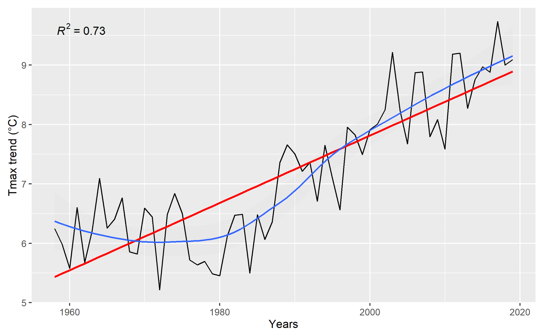
2.2. Climate Data
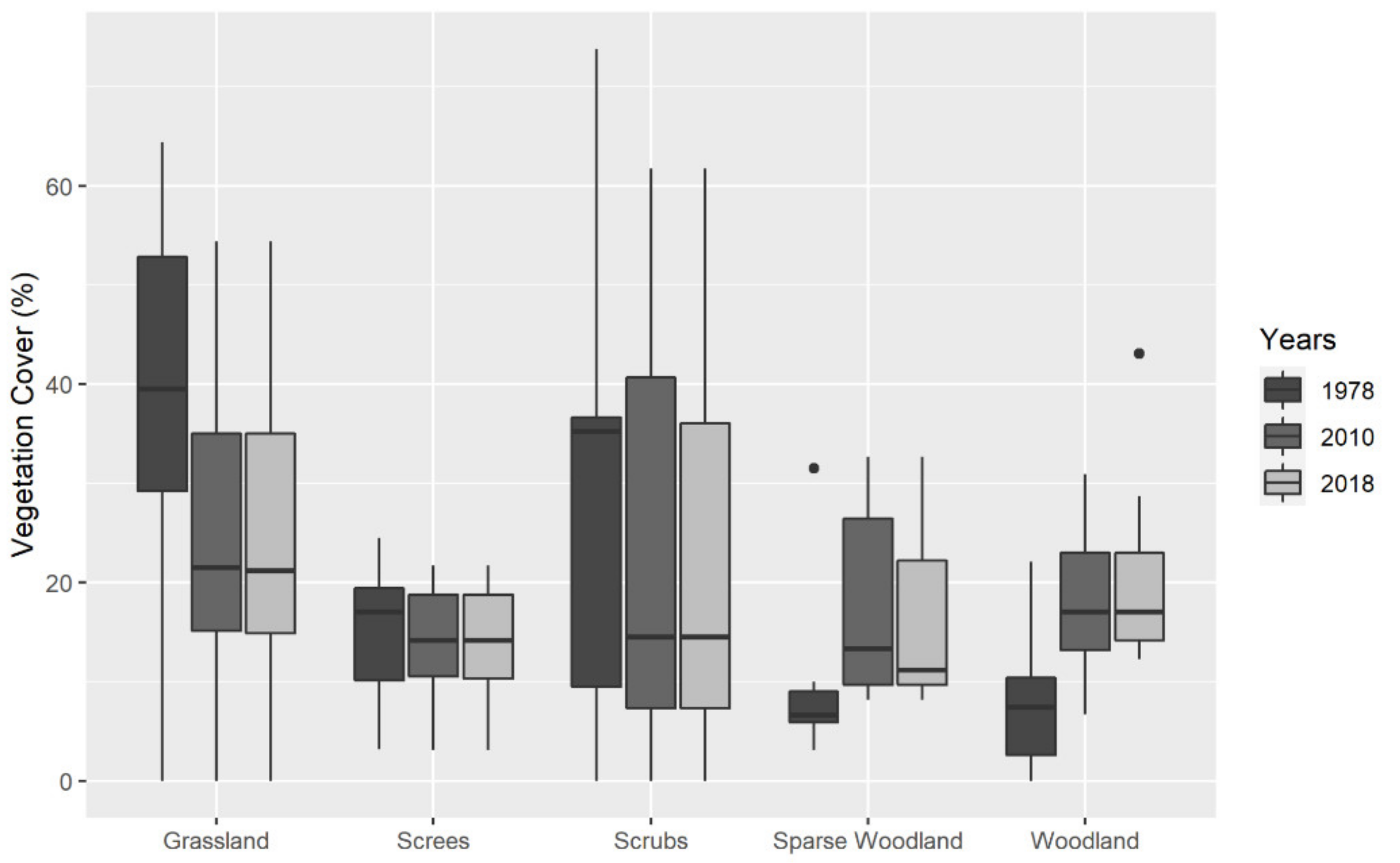
2.3. Vegetation Data
2.4. Butterfly Communities
2.4.1. Ecological Classification of Species
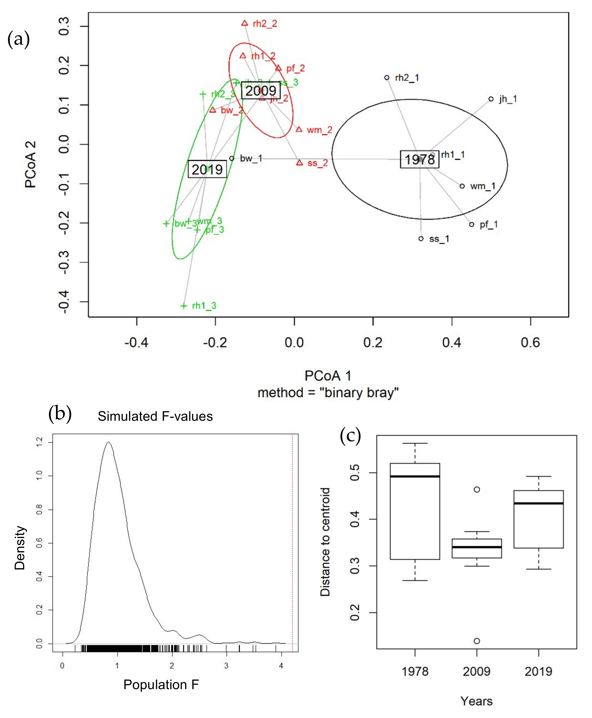
2.4.2. Changes in Butterfly Communities
- -
- were common in all time frames (highest IndVal values in the 1978 + 2009 + 2019 combination);
- -
- abruptly increased their presence during the last decade (highest IndVal in 2009 or 2019 or 2009 + 2019);
- -
- were common in 1978, but strongly suffered during time (highest IndVal in 1978).
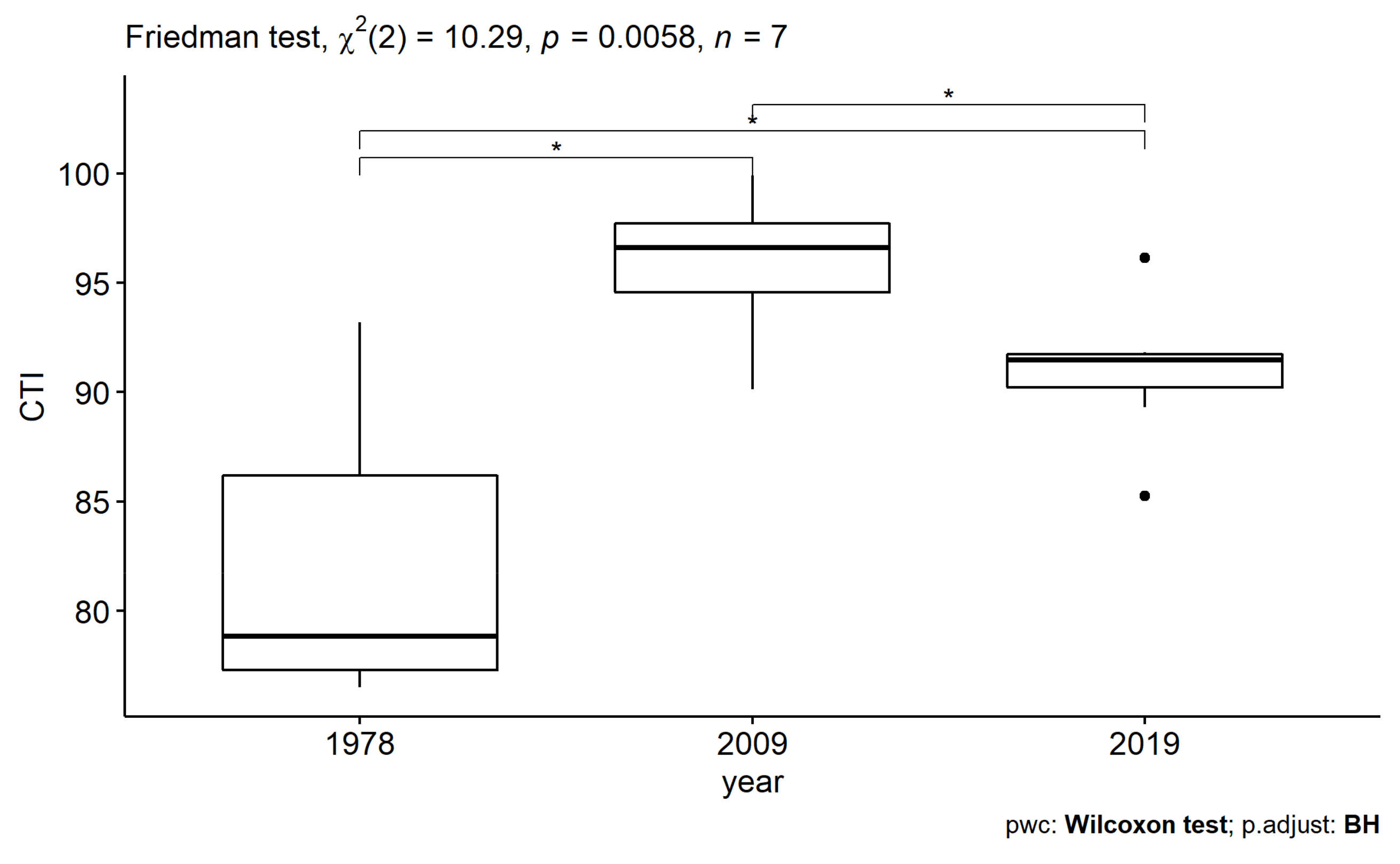
2.4.3. Community Temperature Index
3. Results
3.1. Climate Data
3.2. Vegetational Data
3.3. Changes in Butterfly Communities
3.3.1. Long-Time Series Analysis (1978–2019)
3.3.2. Short-Time Analysis (2009–2019)
4. Discussion
4.1. Large Scale Drivers
4.2. Small Scale Drivers
4.3. Changes in Butterfly Assemblages
5. Conclusions
Supplementary Materials
Author Contributions
Funding
Institutional Review Board Statement
Data Availability Statement
Acknowledgments
Conflicts of Interest
References
- Pachauri, R.K.; Allen, M.R.; Barros, V.R.; Broome, J.; Cramer, W.; Christ, R.; Church, J.A.; Clarke, L.; Dahe, Q.; Dasgupta, P.; et al. Climate Change 2014: Synthesis Report. Contribution of Working Groups I, II and III to the Fifth Assessment Report of the Intergovernmental Panel on Climate Change; Pachauri, R., Meyer, L., Eds.; IPCC: Geneva, Switzerland, 2014. [Google Scholar]
- Hock, R.; Rasul, G.; Adler, C.; Cáceres, B.; Gruber, S.; Hirabayashi, Y.; Jackson, M.; Kääb, A.; Kang, S.; Kutuzov, S.; et al. High Mountain Areas. In Special Report on the Ocean and Cryosphere in a Changing Climate; Portner, H.-O., Roberts, D.C., Masson-Demotte, V., Zhal, P., Tignor, M., Poloczanska, E., Mintenbeck, K., Alegria, A., Nicolai, M., Okem, A., et al., Eds.; IPCC: Geneva, Switzerland, 2019; pp. 131–202. [Google Scholar]
- Guo, D.; Wang, H. CMIP5 Permafrost Degradation Projection: A Comparison among Different Regions. J. Geophys. Res. Atmos. 2016, 121, 4499–4517. [Google Scholar] [CrossRef]
- Qixiang, W.; Wang, M.; Fan, X. Seasonal Patterns of Warming Amplification of High-Elevation Stations across the Globe. Int. J. Clim. 2018, 38, 3466–3473. [Google Scholar] [CrossRef]
- Ciccarelli, N.; von Hardenberg, J.; Provenzale, A.; Ronchi, C.; Vargiu, A.; Pelosini, R. Climate Variability in North-Western Italy during the Second Half of the 20th Century. Glob. Planet. Chang. 2008, 63, 185–195. [Google Scholar] [CrossRef]
- Acquaotta, F.; Fratianni, S.; Garzena, D. Temperature Changes in the North-Western Italian Alps from 1961 to 2010. Theor. Appl. Clim. 2015, 122, 619–634. [Google Scholar] [CrossRef]
- Beniston, M. Mountain Weather and Climate: A General Overview and a Focus on Climatic Change in the Alps. Hydrobiologia 2006, 562, 3–16. [Google Scholar] [CrossRef] [Green Version]
- Wilson, R.J.; Gutiérrez, D.; Gutiérrez, J.; Martínez, D.; Agudo, R.; Monserrat, V.J. Changes to the Elevational Limits and Extent of Species Ranges Associated with Climate Change. Ecol. Lett. 2005, 8, 1138–1146. [Google Scholar] [CrossRef]
- Gobiet, A.; Kotlarski, S.; Beniston, M.; Heinrich, G.; Rajczak, J.; Stoffel, M. 21st Century Climate Change in the European Alps-A Review. Sci. Total Environ. 2014, 493, 1138–1151. [Google Scholar] [CrossRef]
- Rogora, M.; Frate, L.; Carranza, M.L.; Freppaz, M.; Stanisci, A.; Bertani, I.; Bottarin, R.; Brambilla, A.; Canullo, R.; Carbognani, M.; et al. Assessment of Climate Change Effects on Mountain Ecosystems through a Cross-Site Analysis in the Alps and Apennines. Sci. Total Environ. 2018, 624, 1429–1442. [Google Scholar] [CrossRef] [Green Version]
- Winkler, M.; Lamprecht, A.; Steinbauer, K.; Hülber, K.; Theurillat, J.P.; Breiner, F.; Choler, P.; Ertl, S.; Gutiérrez Girón, A.; Rossi, G.; et al. The Rich Sides of Mountain Summits—A Pan-European View on Aspect Preferences of Alpine Plants. J. Biogeogr. 2016, 43, 2261–2273. [Google Scholar] [CrossRef]
- Beniston, M. Climatic Change in Mountain Regions: A Review of Possible Impacts. In Climate Variability and Change in High Elevation Regions: Past, Present & Future. Advances in Global Change Research; Diaz, H.F., Ed.; Springer: Dordrecht, The Netherlands, 2003; Volume 15, pp. 5–31. [Google Scholar] [CrossRef] [Green Version]
- Root, T.L.; Price, J.T.; Hall, K.R.; Schneider, S.H. Fingerprints of Global Warming on Wild Animals and Plants. Nature 2003, 421, 57–60. [Google Scholar] [CrossRef]
- Parmesan, C.; Gaines, S.; Gonzalez, L.; Kaufman, D.M.; Kingsolver, J.; Peterson, A.T.; Sagarin, R. Empirical Perspectives on Species Borders: From Traditional Biogeography to Global Change. Oikos 2005, 108, 58–75. [Google Scholar] [CrossRef] [Green Version]
- Bässler, C.; Müller, J.; Hothorn, T.; Kneib, T.; Badeck, F.; Dziock, F. Estimation of the Extinction Risk for High-Montane Species as a Consequence of Global Warming and Assessment of Their Suitability as Cross-Taxon Indicators. Ecol. Indic. 2010, 10, 341–352. [Google Scholar] [CrossRef]
- Gottfried, M.; Pauli, H.; Futschik, A.; Akhalkatsi, M.; Barančok, P.; Benito Alonso, J.L.; Coldea, G.; Dick, J.; Erschbamer, B.; Fernández Calzado, M.R.; et al. Continent-Wide Response of Mountain Vegetation to Climate Change. Nat. Clim. Chang. 2012, 2, 111–115. [Google Scholar] [CrossRef]
- Falcucci, A.; Maiorano, L.; Boitani, L. Changes in Land-Use/Land-Cover Patterns in Italy and Their Implications for Biodiversity Conservation. Landsc. Ecol. 2007, 22, 617–631. [Google Scholar] [CrossRef]
- Garbarino, M.; Morresi, D.; Urbinati, C.; Malandra, F.; Motta, R.; Sibona, E.M.; Vitali, A.; Weisberg, P.J. Contrasting Land Use Legacy Effects on Forest Landscape Dynamics in the Italian Alps and the Apennines. Landsc. Ecol. 2020, 9. [Google Scholar] [CrossRef]
- Francon, L.; Corona, C.; Till-Bottraud, I.; Carlson, B.Z.; Stoffel, M. Some (Do Not) like It Hot: Shrub Growth Is Hampered by Heat and Drought at the Alpine Treeline in Recent Decades. Am. J. Bot. 2020, 107, 607–617. [Google Scholar] [CrossRef] [Green Version]
- Pellissier, L.; Anzini, M.; Maiorano, L.; Dubuis, A.; Pottier, J.; Vittoz, P.; Guisan, A. Spatial Predictions of Land-Use Transitions and Associated Threats to Biodiversity: The Case of Forest Regrowth in Mountain Grasslands. Appl. Veg. Sci. 2013, 16, 227–236. [Google Scholar] [CrossRef]
- Vittoz, P.; Rulence, B.; Largey, T.; Freléchoux, F. Effects of Climate and Land-Use Change on the Establishment and Growth of Cembran Pine (Pinus cembra L.) over the Altitudinal Treeline Ecotone in the Central Swiss Alps. Arct. Antarct. Alp. Res. 2008, 40, 225–232. [Google Scholar] [CrossRef] [Green Version]
- Vittoz, P.; Bodin, J.; Ungricht, S.; Burga, C.A.; Walther, G.-R. One Century of Vegetation Change on Isla Persa, a Nunatak in the Bernina Massif in the Swiss Alps. J. Veg. Sci. 2008, 19, 671–680. [Google Scholar] [CrossRef]
- Carlson, B.Z.; Renaud, J.; Biron, P.E.; Choler, P. Long-Term Modeling of the Forest-Grassland Ecotone in the French Alps: Implications for Land Management and Conservation. Ecol. Appl. 2014, 24, 1213–1225. [Google Scholar] [CrossRef]
- Kullman, L.; Öberg, L. Post-Little Ice Age Tree Line Rise and Climate Warming in the Swedish Scandes: A Landscape Ecological Perspective. J. Ecol. 2009, 97, 415–429. [Google Scholar] [CrossRef]
- Harsch, M.A.; Hulme, P.E.; McGlone, M.S.; Duncan, R.P. Are Treelines Advancing? A Global Meta-Analysis of Treeline Response to Climate Warming. Ecol. Lett. 2009, 12, 1040–1049. [Google Scholar] [CrossRef]
- Holtmeier, F.K.; Broll, G. Treeline Advance—Driving Processes and Adverse Factors. Landsc. Online 2007, 1, 1–33. [Google Scholar] [CrossRef]
- Wieser, G.; Oberhuber, W.; Gruber, A. Effects of Climate Change at Treeline: Lessons from Space-for-Time Studies, Manipulative Experiments, and Long-Term Observational Records in the Central Austrian Alps. Forests 2019, 10, 508. [Google Scholar] [CrossRef] [Green Version]
- Tasser, E.; Tappeiner, U.; Cernusca, A. Ecological Effects of Land-Use Changes in the European Alps. In Global Change and Mountain Regions. Advances in Global Change Research; Huber, U.M., Bugmann, H.K.M., Reasoner, M.A., Eds.; Springer: Dordrecht, The Netherlands, 2005; p. 23. [Google Scholar] [CrossRef]
- Hinojosa, L.; Napoléone, C.; Moulery, M.; Lambin, E.F. The “Mountain Effect” in the Abandonment of Grasslands: Insights from the French Southern Alps. Agric. Ecosyst. Environ. 2016, 221, 115–124. [Google Scholar] [CrossRef]
- Tasser, E.; Tappeiner, U. Impact of Land Use Changes on Mountain Vegetation. Appl. Veg. Sci. 2002, 5, 173–184. [Google Scholar] [CrossRef]
- Motta, R.; Nola, P. Growth Trends and Dynamics in Sub-alpine Forest Stands in the Varaita Valley (Piedmont, Italy) and Their Relationships with Human Activities and Global Change. J. Veg. Sci. 2001, 12, 219–230. [Google Scholar] [CrossRef]
- Godone, D.; Garbarino, M.; Sibona, E.; Garnero, G.; Godone, F. Progressive Fragmentation of a Traditional Mediterranean Landscape by Hazelnut Plantations: The Impact of CAP over Time in the Langhe Region (NW Italy). Land Use Policy 2014, 36, 259–266. [Google Scholar] [CrossRef] [Green Version]
- Sartorello, Y.; Pastorino, A.; Bogliani, G.; Ghidotti, S.; Viterbi, R.; Cerrato, C. The Impact of Pastoral Activities on Animal Biodiversity in Europe: A Systematic Review and Meta-Analysis. J. Nat. Conserv. 2020, 56, 125863. [Google Scholar] [CrossRef]
- Vittoz, P.; Cherix, D.; Gonseth, Y.; Lubini, V.; Maggini, R.; Zbinden, N.; Zumbach, S. Climate Change Impacts on Biodiversity in Switzerland: A Review. J. Nat. Conserv. 2013, 21, 154–162. [Google Scholar] [CrossRef]
- Carlson, B.Z.; Randin, C.F.; Boulangeat, I.; Lavergne, S.; Thuiller, W.; Choler, P. Working toward Integrated Models of Alpine Plant Distribution. Alp. Bot. 2013, 123, 41–53. [Google Scholar] [CrossRef] [PubMed] [Green Version]
- Butler, D.R.; Malanson, G.P.; Walsh, S.J.; Fagre, D.B. Influences of Geomorphology and Geology on Alpine Treeline in the American West—More Important than Climatic Influences? Phys. Geogr. 2007, 28, 434–450. [Google Scholar] [CrossRef] [Green Version]
- Körner, C. Alpine Plant Life: Functional Plant Ecology of High Mountain Ecosystems; Springer: Berlin/Heidelberg, Germany, 2003. [Google Scholar] [CrossRef]
- Körner, C.; Ohsawa, M. Mountain systems. In Ecosystems and Human Well-Being: Current State and Trends; Hassan, R., Scholes, R., Ash, N., Eds.; Island Press: London, UK, 2005. [Google Scholar]
- Holyoak, M.; Heath, S.K. The Integration of Climate Change, Spatial Dynamics, and Habitat Fragmentation: A Conceptual Overview. Integr. Zool. 2016, 11, 40–59. [Google Scholar] [CrossRef] [PubMed] [Green Version]
- Magurran, A.E.; Baillie, S.R.; Buckland, S.T.; Dick, J.M.P.; Elston, D.A.; Scott, E.M.; Smith, R.I.; Somerfield, P.J.; Watt, A.D. Long-Term Datasets in Biodiversity Research and Monitoring: Assessing Change in Ecological Communities through Time. Trends Ecol. Evol. 2010, 25, 574–582. [Google Scholar] [CrossRef]
- Rödder, D.; Schmitt, T.; Gros, P.; Ulrich, W.; Habel, J.C. Climate change drives mountain butterflies towards the summits. Sci. Rep. 2021, 11, 1–12. [Google Scholar] [CrossRef]
- Dennis, R.L. Butterflies and Climate Change; University Press: Manchester, UK, 1993. [Google Scholar]
- Roth, T.; Plattner, M.; Amrhein, V. Plants, Birds and Butterflies: Short-Term Responses of Species Communities to Climate Warming Vary by Taxon and with Altitude. PLoS ONE 2014, 9, e82490. [Google Scholar] [CrossRef]
- Parmesan, C. Ecological and Evolutionary Responses to Recent Climate Change. Annu. Rev. Ecol. Evol. Syst. 2006, 37, 637–669. [Google Scholar] [CrossRef] [Green Version]
- Parmesan, C.; Yohe, G. A Globally Coherent Fingerprint of Climate Change Impacts across Natural Systems. Nature 2003, 42, 37–42. [Google Scholar] [CrossRef]
- Devictor, V.; van Swaay, C.; Brereton, T.; Brotons, L.; Chamberlain, D.; Heliölö, J.; Herrando, S.; Julliard, R.; Kuussaari, M.; Lindström, Å.; et al. Differences in the Climatic Debts of Birds and Butterflies at a Continental Scale. Nat. Clim. Chang. 2012, 2, 121–124. [Google Scholar] [CrossRef]
- Thomas, J.A.; Telfer, M.G.; Roy, D.B.; Preston, C.D.; Greenwood, J.J.D.; Asher, J.; Fox, R.; Clarke, R.T.; Lawton, J.H. Comparative Losses of British Butterflies, Birds, and Plants and the Global Extinction Crisis. Science 2004, 303, 1879–1881. [Google Scholar] [CrossRef] [Green Version]
- Hellman, J.J. Butterflies as Model Systems for Understanding and Predicting Climate Change. In Wildlife Responses to Climate Change: North American Case Studies; Schneider, S.H., Root, T.L., Eds.; Island Pres: Washington, DC, USA, 2002; pp. 93–126. [Google Scholar]
- Viterbi, R.; Cerrato, C.; Bionda, R.; Provenzale, A. Effects of Temperature Rise on Multi-Taxa Distributions in Mountain Ecosystems. Diversity 2020, 12, 210. [Google Scholar] [CrossRef]
- Roy, D.B.; Sparks, T.H. Phenology of British Butterflies and Climate Change. Glob. Chang. Biol. 2000, 6, 407–416. [Google Scholar] [CrossRef]
- Schilthuizen, M.; Kellermann, V. Contemporary Climate Change and Terrestrial Invertebrates: Evolutionary versus Plastic Changes. Evol. Appl. 2014, 7, 56–67. [Google Scholar] [CrossRef]
- Illán, J.G.; Gutiérrez, D.; Díez, S.B.; Wilson, R.J. Elevational Trends in Butterfly Phenology: Implications for Species Responses to Climate Change. Evol. Appl. 2012, 37, 134–144. [Google Scholar] [CrossRef]
- Stefanescu, C.; Penuelas, J.; Filella, I. Effects of Climatic Change on the Phenology of Butterflies in the Northwest Mediterranean Basin. Glob. Chang. Biol. 2003, 9, 1494–1506. [Google Scholar] [CrossRef]
- Zografou, K.; Grill, A.; Wilson, R.J.; Halley, J.M.; Adamidis, G.C.; Kati, V. Butterfly Phenology in Mediterranean Mountains Using Space-for-Time Substitution. Ecol. Evol. 2020, 10, 928–939. [Google Scholar] [CrossRef]
- Altermatt, F. Climatic Warming Increases Voltinism in European Butterflies and Moths. Proc. R. Soc. B Boil. Sci. 2010, 277, 1281–1287. [Google Scholar] [CrossRef] [Green Version]
- Hill, J.K.; Thomas, C.D.; Fox, R.; Telfer, M.G.; Willis, S.G.; Asher, J.; Huntley, B. Responses of Butterflies to Twentieth Century Climate Warming: Implications for Future Ranges. Proc. R. Soc. B Boil. Sci. 2002, 269, 2163–2171. [Google Scholar] [CrossRef] [Green Version]
- Warren, M.S.; Hill, J.K.; Thomas, J.A.; Asher, J.; Fox, R.; Huntley, B.; Roy, D.B.; Telfer, M.G.; Jeffcoate, S.; Harding, P.; et al. Rapid Responses of British Butterflies to Opposing Forces of Climate and Habitat Change. Nature 2001, 414, 65–69. [Google Scholar] [CrossRef] [Green Version]
- Stuhldreher, G.; Fartmann, T. Threatened Grassland Butterflies as Indicators of Microclimatic Niches along an Elevational Gradient—Implications for Conservation in Times of Climate Change. Ecol. Indic. 2018, 94, 83–98. [Google Scholar] [CrossRef]
- Habel, J.C.; Segerer, A.; Ulrich, W.; Torchyk, O.; Weisser, W.W.; Schmitt, T. Butterfly Community Shifts over Two Centuries. Conserv. Biol. 2016, 30, 754–762. [Google Scholar] [CrossRef]
- Cerrato, C.; Rocchia, E.; Brunetti, M.; Bionda, R.; Bassano, B.; Provenzale, A.; Bonelli, S.; Viterbi, R. Butterfly Distribution along Altitudinal Gradients: Temporal Changes over a Short Time Period. Nat. Conserv. 2019, 34, 91–118. [Google Scholar] [CrossRef] [Green Version]
- Bonelli, S.; Barbero, F.; Casacci, L.P.; Cerrato, C.; Balletto, E. The Butterfly Fauna of the Italian Maritime Alps: Results of the EDIT Project. Zoosystema 2015, 37, 139–167. [Google Scholar] [CrossRef] [Green Version]
- Balletto, E.; Bonelli, S.; Cassulo, L.A.; Meregalli, M.; Tontini, L. Italy. In Prime Butterfly Areas in Europe: Priority Sites for Conservation; van Swaay, C.A.M., Warren, M.S., Eds.; Ministry of Agriculture, Nature Management and Fisheries: Wageningen, The Netherlands, 2003; pp. 328–356. [Google Scholar]
- Balletto, E.; Barberis, G.; Toso, G.G. Aspetti dell’ecologia dei lepidotteri ropaloceri nei consorzi erbacei delle Alpi italian. In Quaderni Sulla “Struttura Delle Zoocenosi Terrestri"; CNR: Roma, Italy, 1982; pp. 11–95. [Google Scholar]
- Kalnay, E. Atmospheric Modeling, Data Assimilation and Predictability; Cambridge University Press: Cambridge, UK, 2002. [Google Scholar]
- Ronchi, C.; Luigi, C.D.; Ciccarelli, N.; Loglisci, N. Development of a Daily Gridded Climatological Air Temperature Dataset Based on a Optimal Interpolation of ERA-40 Reanalysis Downscaling and a Local High Resolution Thermometers Network. In Proceedings of the 8th EMS Annual Meeting and 7th European Conference on Applied Climatology, Amsterdam, The Netherlands, 29 September–3 October 2008. [Google Scholar]
- Uboldi, F.; Lussana, C.; Salvati, M. Three-Dimensional Spatial Interpolation of Surface Meteorological Observations from High-Resolution Local Networks. Meteorol. Appl. 2009, 101, 331–345. [Google Scholar] [CrossRef]
- Rolland, C. Spatial and Seasonal Variations of Air Temperature Lapse Rates in Alpine Regions. J. Clim. 2003, 16, 1032–1046. [Google Scholar] [CrossRef] [Green Version]
- Cleveland, R.B.; Cleveland, W.S.; McRae, J.E.; Terpenning, I. STL: A Seasonal-Trend Decomposition Procedure Based on Loess. J. Off. Stat. 1990, 6, 3–73. [Google Scholar]
- Hill, J.K.; Thomas, C.D.; Huntley, B. Modeling present and potential future ranges of European butterflies using climate response surfaces. In Butterflies. Ecology and Evolution Taking Flight; Bogs, C., Watt, W., Ehrlich, P., Eds.; The University of Chicago Press: Chicago, IL, USA, 2003; pp. 149–167. [Google Scholar]
- Heikkinen, R.K.; Luoto, M.; Leikola, N.; Pöyry, J.; Settele, J.; Kudrna, O.; Marmion, M.; Fronzek, S.; Thuiller, W. Assessing the Vulnerability of European Butterflies to Climate Change Using Multiple Criteria. Biodivers. Conserv. 2010, 19, 695–723. [Google Scholar] [CrossRef]
- Martin, Y.; van Dyck, H.; Legendre, P.; Settele, J.; Schweiger, O.; Harpke, A.; Wiemers, M.; Ameztegui, A.; Titeux, N. A Novel Tool to Assess the Effect of Intraspecific Spatial Niche Variation on Species Distribution Shifts under Climate Change. Glob. Ecol. Biogeogr. 2020, 29, 590–602. [Google Scholar] [CrossRef]
- Pollard, E.; Yates, T.J. Monitoring Butterflies for Ecology and Conservation; Chapam & Hall: London, UK, 1993. [Google Scholar]
- Balletto, E.; Kudrna, O. Some Aspects of the Conservation of the Butterflies (Lepidoptera: Papilionoidea) in Italy, with Recommendations for the Future Strategy. Boll. Soc. Entomol. Ital. 1985, 117, 39–59. [Google Scholar]
- Maciel, E.A. An Index for Assessing the Rare Species of a Community. Ecol. Indic. 2021, 124. [Google Scholar] [CrossRef]
- Rabinowitz, D. Seven forms of rarity. In The Biological Aspect of Rare Plant Conservation; Synge, H., Ed.; John Wiley & Sons Ltd.: Somerset, NJ, USA, 1981; pp. 205–217. [Google Scholar]
- Anderson, M.J. A New Method for Non-Parametric Multivariate Analysis of Variance. Austral Ecol. 2001, 26, 32–46. [Google Scholar]
- McArdle, B.H.; Anderson, M.J. Fitting Multivariate Models to Community Data: A Comment on Distance-Based Redundancy Analysis. Ecol. Soc. Am. 2001, 82, 290–297. [Google Scholar] [CrossRef]
- Oksanen, A.J.; Blanchet, F.G.; Friendly, M.; Kindt, R.; Legendre, P.; Mcglinn, D.; Minchin, P.R.; Hara, R.B.O.; Simpson, G.L.; Solymos, P.; et al. Vegan: Community Ecology Package. In R Package Version 2.0-2; R Package: Vienn, Austria, 2012. [Google Scholar]
- Dufrêne, M.; Legendre, P. DufreneLegendre1997_species Assemblages and Indicator Species_the Need for Flexible Asymmetrical Approach.PDF. Ecol. Monogr. 1997, 67, 345–366. [Google Scholar]
- de Cáceres, M.; Legendre, P. Associations between Species and Groups of Sites: Indices and Statistical Inference. Ecology 2009, 90, 3566–3574. [Google Scholar] [CrossRef]
- Tayleur, C.M.; Devictor, V.; Gaüzère, P.; Jonzén, N.; Smith, H.G.; Lindström, Å. Regional Variation in Climate Change Winners and Losers Highlights the Rapid Loss of Cold-Dwelling Species. Divers. Distrib. 2016, 22, 468–480. [Google Scholar] [CrossRef] [Green Version]
- Balletto, E.; Bonelli, S.; Cassulo, L. Insecta Lepidoptera Papilionoidea. In Checklist and Distribution of the Italian Fauna. 10,000 Terrestrial and Freshwater Species; Ruffo, S., Stoch, F., Eds.; Memorie del Museo Civico di Storia Naturale di Verona, 2° serie, Sez. Scienze della Vita; Comune di Verona: Verona, Italy, 2007; pp. 257–261. [Google Scholar]
- Ruffo, S.; Stoch, F. Checklist e Distribuzione Della Fauna Italiana. Ministero della transizione ecologica: Roma, Italy, 2005; Volume 16, ISBN 8889230037. [Google Scholar]
- Metz, M.; Rocchini, D.; Neteler, M. Surface Temperatures at the Continental Scale: Tracking Changes with Remote Sensing at Unprecedented Detail. Remote Sens. 2014, 6, 3822–3840. [Google Scholar] [CrossRef] [Green Version]
- Ernakovich, J.G.; Hopping, K.A.; Berdanier, A.B.; Simpson, R.T.; Kachergis, E.J.; Steltzer, H.; Wallenstein, M.D. Predicted Responses of Arctic and Alpine Ecosystems to Altered Seasonality under Climate Change. Glob. Chang. Biol. 2014, 20, 3256–3269. [Google Scholar] [CrossRef]
- Pateman, R.M.; Hill, J.K.; Roy, D.B.; Fox, R.; Thomas, C.D. Temperature-Dependent Alterations in Host Use Drive Rapid Range Expansion in a Butterfly. Science 2012, 336, 1028–1030. [Google Scholar] [CrossRef]
- Chesson, P. Mechanism of Maintenance of Species Diversity. Annu. Rev. Ecol. Syst. 2000, 31, 343–358. [Google Scholar] [CrossRef] [Green Version]
- Case, B.S.; Duncan, R.P. A Novel Framework for Disentangling the Scale-Dependent Influences of Abiotic Factors on Alpine Treeline Position. Ecography 2014, 37, 838–851. [Google Scholar] [CrossRef]
- Mcneely, J.A. Climate Change and Biological Diversity: Policy Implications. In Landscape Ecological Impacts of Climate Change; de Boer, M.M., de Groot, R.S., Eds.; IOS Press: Amsterdam, The Netherlands, 1990; pp. 406–428. [Google Scholar]
- Angert, A.L.; Crozier, L.G.; Rissler, L.J.; Gilman, S.E.; Tewksbury, J.J.; Chunco, A.J. Do Species’ Traits Predict Recent Shifts at Expanding Range Edges? Ecol. Lett. 2011, 14, 677–689. [Google Scholar] [CrossRef]
- Parmesan, C.; Ryrholm, N.; Stefanescu, C.; Hill, J.K.; Thomas, C.D.; Descimon, H.; Huntley, B.; Kaila, L.; Kullberg, J.; Tammaru, T.; et al. Poleward Shifts in Geographical Ranges of Butterfly Species Associated with Regional Warming. Nature 1999, 399, 579–583. [Google Scholar] [CrossRef]
- Wilson, R.J.; Gutiérrez, D.; Gutiérrez, J.; Monserrat, V.J. An Elevational Shift in Butterfly Species Richness and Composition Accompanying Recent Climate Change. Glob. Chang. Biol. 2007, 13, 1873–1887. [Google Scholar] [CrossRef]
- Cini, A.; Barbero, F.; Bonelli, S.; Bruschini, C.; Casacci, L.P.; Piazzini, S.; Scalercio, S.; Dapporto, L. The Decline of the Charismatic Parnassius Mnemosyne (L.) (Lepidoptera: Papilionidae) in a Central Italy National Park: A Call for Urgent Actions. J. Insect Biodivers. 2020, 16, 47–54. [Google Scholar] [CrossRef]
- Olden, J.D.; Rooney, T.P. On Defining and Quantifying Biotic Homogenization. Glob. Ecol. Biogeogr. 2006, 15, 113–120. [Google Scholar] [CrossRef]
- González-Megías, A.; Menéndez, R.; Roy, D.; Brereton, T.; Thomas, C.D. Changes in the Composition of British Butterfly Assemblages over Two Decades. Glob. Chang. Biol. 2008, 14, 1464–1474. [Google Scholar] [CrossRef]
- Gámez-Virués, S.; Perović, D.J.; Gossner, M.M.; Börschig, C.; Blüthgen, N.; de Jong, H.; Simons, N.K.; Klein, A.M.; Krauss, J.; Maier, G.; et al. Landscape Simplification Filters Species Traits and Drives Biotic Homogenization. Nat. Commun. 2015, 6, 8568. [Google Scholar] [CrossRef]
- Ekroos, J.; Heliölä, J.; Kuussaari, M. Homogenization of Lepidopteran Communities in Intensively Cultivated Agricultural Landscapes. J. Appl. Ecol. 2010, 47, 459–467. [Google Scholar] [CrossRef]
- Mckinney, M.L.; Lockwood, J.L. Taxonomic and Ecological Enhancement of Homogenization. Tree 1999, 5347, 450–453. [Google Scholar] [CrossRef]
- Bolotov, I.N. Long-Term Changes in the Fauna of Diurnal Lepidopterans (Lepidoptera, Diurna) in the Northern Taiga Subzone of the Western Russian Plain. Russ. J. Ecol. 2004, 35, 117–123. [Google Scholar] [CrossRef]
- Kuussaari, M.; Heliölä, J.; Pöyry, J.; Saarinen, K. Contrasting Trends of Butterfly Species Preferring Semi-Natural Grasslands, Field Margins and Forest Edges in Northern Europe. J. Insect Conserv. 2007, 11, 351–366. [Google Scholar] [CrossRef]
- Balandier, P.; Marquier, A.; Casella, E.; Kiewitt, A.; Coll, L.; Wehrlen, L.; Harmer, R. Architecture, Cover and Light Interception by Bramble (Rubus Fruticosus): A Common Understorey Weed in Temperate Forests. Forestry 2013, 86, 39–46. [Google Scholar] [CrossRef] [Green Version]
- Jandt, U.; von Wehrden, H.; Bruelheide, H. Exploring Large Vegetation Databases to Detect Temporal Trends in Species Occurrences. J. Veg. Sci. 2011, 22, 957–972. [Google Scholar] [CrossRef]
- Melero, Y.; Stefanescu, C.; Pino, J. General Declines in Mediterranean Butterflies over the Last Two Decades Are Modulated by Species Traits. Biol. Conserv. 2016, 201, 336–342. [Google Scholar] [CrossRef] [Green Version]
- Warren, M.S.; Maes, D.; van Swaay, C.A.; Goffart, P.; Van Dyck, H.; Bourn, N.A.; Wynhoff, I.; Hoare, D.; Ellis, S. The decline of butterflies in Europe: Problems, significance, and possible solutions. Proc. Natl. Acad. Sci. USA 2021, 118, e2002551117. [Google Scholar] [CrossRef]
- Boggs, C.L.; Murphy, D.D. Community Composition in Mountain Ecosystems: Climatic Determinants of Montane Butterfly Distributions. Glob. Ecol. Biogeogr. Lett. 1997, 6, 39–48. [Google Scholar] [CrossRef]
- Shreeve, T.G. Butterfly mobility. In Ecology and Conservation of Butterflies; Pullin, A.S., Ed.; Springer: Dordrecht, The Netherlands, 1995. [Google Scholar]
- Krauss, J.; Steffan-Dewenter, I.; Tscharntke, T. Local Species Immigration, Extinction, and Turnover of Butterflies in Relation to Habitat Area and Habitat Isolation. Oecologia 2003, 137, 591–602. [Google Scholar] [CrossRef]
- Estrada, A.; Morales-Castilla, I.; Caplat, P.; Early, R. Usefulness of Species Traits in Predicting Range Shifts. Trends Ecol. Evol. 2016, 31, 190–203. [Google Scholar] [CrossRef] [Green Version]
- Pryde, E.C.; Nimmo, D.G.; Holland, G.J.; Watson, S.J. Species’ Traits Affect the Occurrence of Birds in a Native Timber Plantation Landscape. Anim. Conserv. 2016, 19, 526–538. [Google Scholar] [CrossRef]
- Walther, G.R. Community and Ecosystem Responses to Recent Climate Change. Philos. Trans. R. Soc. B Biol. Sci. 2010, 365, 2019–2024. [Google Scholar] [CrossRef] [PubMed]
- le Roux, P.C.; McGeoch, M.A. Rapid Range Expansion and Community Reorganization in Response to Warming. Glob. Chang. Biol. 2008, 14, 2950–2962. [Google Scholar] [CrossRef]
- Wilson, R.; Gutierrez, D. Effects of climate change on the elevational limits of species ranges. In Ecological Consequences of Climate Change; Beever, E.A., Belant, J.L., Eds.; CRC Press: Boca Raton, FL, USA, 2012. [Google Scholar]


| Habitat Type | Code | Elevation (m) | Coordinates |
|---|---|---|---|
| Beech-wood clearings | Bw | 1250 | 44°12′56.62″−7°16′48.2″ |
| Rhododendron heathland | rh1 | 1600 | 44°12′11.62″−7°14′53.81″ |
| Rhododendron heathland | rh2 | 1750 | 44°12′7.75″−7°14′30.27″ |
| Wet acid grassland | Wm | 1750 | 44°12′2.77″−7°14′24.07″ |
| Subalpine screes | Ss | 1900 | 44°11′21.91″−7°13′18.34″ |
| Juniperus heathland | Jh | 1800 | 44°11′51.2″−7°13′38.32″ |
| Pastures with Festuca paniculata | Pf | 1750 | 44°12′6.72″−7°14′23.99″ |
| 1978 | 2009 | 2019 | |
|---|---|---|---|
| T mean | 4.07 | 5.19 | 5.67 |
| T mean (DJF) | −2.34 | −3.06 | −0.07 |
| T mean (MAM) | 1.71 | 4.21 | 2.49 |
| T mean (JJA) | 10.77 | 13.25 | 14.12 |
| MTCO (Jan) | −3.65 | −3.58 | −2.85 |
| dd (Feb) | 0 | 0 | 88.13 |
| dd (Apr) | 7.14 | 5.7 | 241.62 |
| dd (Jun) | 277.35 | 676.6 | 243.98 |
| dd (Aug) | 1100.48 | 1824.47 | 3734.76 |
| Species | 1978 | 2009 | 2019 | 1978–2009 | 1978–2019 | 2009–2019 | All | p-Value | |
|---|---|---|---|---|---|---|---|---|---|
| Anthocharis cardamines | 0.845 | 0.000 | 0.000 | 0.598 | 0.598 | 0.000 | 0.488 | 0.004 | 1978 |
| Parnassius mnemosyne | 0.756 | 0.000 | 0.000 | 0.535 | 0.535 | 0.000 | 0.436 | 0.015 | |
| Pieris bryoniae | 0.655 | 0.000 | 0.000 | 0.463 | 0.463 | 0.000 | 0.378 | 0.074 | |
| Pontia callidice | 0.655 | 0.000 | 0.000 | 0.463 | 0.463 | 0.000 | 0.378 | 0.083 | |
| Pyrgus carthami | 0.845 | 0.000 | 0.000 | 0.598 | 0.598 | 0.000 | 0.488 | 0.004 | |
| Aricia nicias | 0.134 | 0.668 | 0.267 | 0.567 | 0.283 | 0.661 | 0.617 | 0.135 | 2009 |
| Parnassius apollo | 0.154 | 0.617 | 0.154 | 0.546 | 0.218 | 0.546 | 0.535 | 0.264 | |
| Polyommatus icarus | 0.154 | 0.772 | 0.000 | 0.655 | 0.109 | 0.546 | 0.535 | 0.017 | |
| Polyommatus bellargus | 0.000 | 0.000 | 0.655 | 0.000 | 0.463 | 0.463 | 0.378 | 0.075 | 2019 |
| Eumedonia eumedon | 0.668 | 0.401 | 0.000 | 0.756 | 0.472 | 0.283 | 0.617 | 0.054 | |
| Lycaena eurydame | 0.617 | 0.309 | 0.000 | 0.655 | 0.436 | 0.218 | 0.535 | 0.147 | 1978–2009 |
| Melitaea athalia | 0.286 | 0.571 | 0.143 | 0.606 | 0.303 | 0.505 | 0.577 | 0.605 | |
| Plebejus argus | 0.571 | 0.429 | 0.000 | 0.707 | 0.404 | 0.303 | 0.577 | 0.125 | |
| Polyommatus escheri | 0.286 | 0.571 | 0.143 | 0.606 | 0.303 | 0.505 | 0.577 | 0.612 | |
| Vanessa cardui | 0.378 | 0.756 | 0.000 | 0.802 | 0.267 | 0.535 | 0.655 | 0.027 | |
| Argynnis niobe | 0.000 | 0.429 | 0.571 | 0.303 | 0.404 | 0.707 | 0.577 | 0.124 | 2009–2019 |
| Argynnis paphia | 0.000 | 0.630 | 0.504 | 0.445 | 0.356 | 0.802 | 0.655 | 0.021 | |
| Brenthis daphne | 0.000 | 0.630 | 0.504 | 0.445 | 0.356 | 0.802 | 0.655 | 0.019 | |
| Coenonympha arcania | 0.000 | 0.571 | 0.429 | 0.404 | 0.303 | 0.707 | 0.577 | 0.105 | |
| Erebia ligea | 0.143 | 0.429 | 0.429 | 0.404 | 0.404 | 0.606 | 0.577 | 0.607 | |
| Lycaena alciphron | 0.143 | 0.429 | 0.429 | 0.404 | 0.404 | 0.606 | 0.577 | 0.600 | |
| Lycaena virgaureae | 0.275 | 0.642 | 0.642 | 0.648 | 0.648 | 0.907 | 0.900 | 0.009 | |
| Satyrus ferula | 0.114 | 0.570 | 0.570 | 0.483 | 0.483 | 0.806 | 0.724 | 0.036 | |
| Speyeria aglaja | 0.239 | 0.478 | 0.478 | 0.507 | 0.507 | 0.676 | 0.690 | NA | All |
| Boloria titania | 0.478 | 0.478 | 0.239 | 0.676 | 0.507 | 0.507 | 0.690 | NA | |
| Erebia albergana | 0.567 | 0.661 | 0.283 | 0.869 | 0.601 | 0.668 | 0.873 | NA | |
| Erebia euryale | 0.314 | 0.629 | 0.419 | 0.667 | 0.519 | 0.741 | 0.787 | NA | |
| Erebia melampus | 0.267 | 0.267 | 0.535 | 0.378 | 0.567 | 0.567 | 0.617 | NA | |
| Lasiommata maera | 0.359 | 0.598 | 0.239 | 0.676 | 0.423 | 0.592 | 0.690 | NA | |
| Pieris rapae | 0.550 | 0.458 | 0.550 | 0.713 | 0.778 | 0.713 | 0.900 | NA | |
| Thymelicus lineola | 0.239 | 0.598 | 0.359 | 0.592 | 0.423 | 0.676 | 0.690 | NA |
Publisher’s Note: MDPI stays neutral with regard to jurisdictional claims in published maps and institutional affiliations. |
© 2021 by the authors. Licensee MDPI, Basel, Switzerland. This article is an open access article distributed under the terms and conditions of the Creative Commons Attribution (CC BY) license (https://creativecommons.org/licenses/by/4.0/).
Share and Cite
Bonelli, S.; Cerrato, C.; Barbero, F.; Boiani, M.V.; Buffa, G.; Casacci, L.P.; Fracastoro, L.; Provenzale, A.; Rivella, E.; Zaccagno, M.; et al. Changes in Alpine Butterfly Communities during the Last 40 Years. Insects 2022, 13, 43. https://doi.org/10.3390/insects13010043
Bonelli S, Cerrato C, Barbero F, Boiani MV, Buffa G, Casacci LP, Fracastoro L, Provenzale A, Rivella E, Zaccagno M, et al. Changes in Alpine Butterfly Communities during the Last 40 Years. Insects. 2022; 13(1):43. https://doi.org/10.3390/insects13010043
Chicago/Turabian StyleBonelli, Simona, Cristiana Cerrato, Francesca Barbero, Maria Virginia Boiani, Giorgio Buffa, Luca Pietro Casacci, Lorenzo Fracastoro, Antonello Provenzale, Enrico Rivella, Michele Zaccagno, and et al. 2022. "Changes in Alpine Butterfly Communities during the Last 40 Years" Insects 13, no. 1: 43. https://doi.org/10.3390/insects13010043
APA StyleBonelli, S., Cerrato, C., Barbero, F., Boiani, M. V., Buffa, G., Casacci, L. P., Fracastoro, L., Provenzale, A., Rivella, E., Zaccagno, M., & Balletto, E. (2022). Changes in Alpine Butterfly Communities during the Last 40 Years. Insects, 13(1), 43. https://doi.org/10.3390/insects13010043