Theoretical Study on Compliance and Stability of Active Gas-Static Journal Bearing with Output Flow Rate Restriction and Damping Chambers

Abstract

The design is considered and theoretical research of operability of the active radial gas-static bearing with restrictors of output flow rate in the form of mobile rings with an elastic supports and the dampers working by Helmholtz acoustic resonator principle is done. The mathematical model of the bearing dynamics and method of calculating its degree of stability are developed. The device is steady against vibrations; it has smaller power consumption compared to the known devices with input regulators, a zero and negative compliance of a gas-lubricated film.

1. Introduction

One of the drawbacks of active gas-static bearings of zero and negative compliance with input regulators of lubricant flow is the high energy consumption. The flow rate in these designs can be several times higher than that of conventional bearings [1,2,3].

In [3], an alternative principle of flow control, which is the use of special devices to limit the output lubricant flow, was proposed. Hydrostatic bearings of this type are also able to provide non-positive compliance; however, their flow rates correspond to conventional bearings, which is significantly less, and this ensures their energy efficiency [4]. It can be expected that similar designs of gas-static bearings will also have similar operational properties.

It is possible to improve the dynamic characteristics of the thrust bearing by means of improvements aimed at reducing the volume of the bearing lubricating film and increasing its damping capacity [5,6].

The main problem of creating effective gas-static bearings with active flow rate is to ensure their stable operation, since a decrease of compliance is accompanied by an increase in factors contributing to deterioration in the quality of its dynamics. The weakening of these factors can be achieved by installing special damping devices [7]. Piezoelectric actuators are used for active runout compensation in aerostatic bearings [8]. Improving performance is possible with squeeze film damping [9]. Contactless gas bearing stabilization devices are used [10]. To improve the quality of the dynamics of bearings with gas pressure regulators, resonator chambers and Helmholtz resonators are successfully used [11,12].

The article presents the results of a theoretical study on the quality of the dynamics of a double-row symmetrical gas-static bearing with a limitation of the output flow of the lubricant, in which a device containing a blind gap and non-flowing resonator chambers is used to improve its dynamic characteristics.

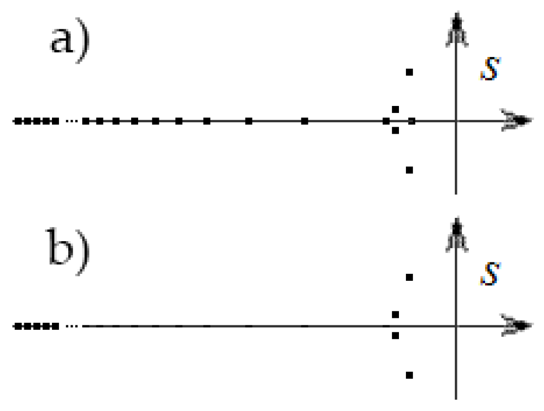
2. Design of the Bearing and the Principle of its Operation

The layout of a circular type bearing with a throttling elastic orifice and damping annular diaphragms is shown in Figure 1.

Figure 1 shows a bearing longitudinal section. The design includes a shaft 2 and a housing 1, where the input feeding slotted channels 3 are made. On the inner sides of the housing ends there are elastic rings 4 to which the rigid rings 5 are attached. The outer cylindrical surfaces of the rings 5 and the housing 1 form slotted gaps 6 of thickness h_p, and their inner surfaces together with the shaft surface form the end bearing layer 8 of thickness h_t. The inner surface of the housing 1 and the surface of the shaft 2 create a gap 7 of the main bearing layer of thickness h. On the outer surface of the rings 5, at their ends, damping chambers 9 of volume V_p are uniformly arranged around the circle, operating on the principle of Helmholtz acoustic resonator.

The bearing operates as follows. The gas lubricant supplied under pressure p_s, having overcome the hydraulic resistance of the channels 3, enters a thin lubricating gap 6 and bearing lubricating clearances 7 and 8 under pressure p_t, and then flows out of the bearing. The hydraulic forces created by the pressure on the surface of the rings 5 are balanced by the elastic material deformation resistance of the elastic rings 4. The integral reaction of the pressure forces on the rings 5 in the gaps 6 is always greater than the corresponding reaction from the gaps 8, as can be seen by the analysis of the corresponding pressure distribution diagrams. For this reason, during the bearing’s operation, the rings 5 will make a movement that is opposite to the external force vector f, creating an obstacle to the outflow of lubricant from the bearing, therefore increasing the hydraulic force acting on the shaft displaced under the load and reducing the bearing compliance.

3. Statement of the Problem and Method of Its Solution

When simulating the operation of the bearing, it was assumed that during the movement the axes of the housing, shaft, and movable rings 5 are parallel. The calculations were carried out using dimensionless quantities. The scales are as follows: the shaft radius r₀ is for linear dimensions, the ambient pressure p_a is for pressures, πr₀²p_a is for forces, h₀³p_a²/24µRT is for mass gas flow rates, h₀ is for gaps and eccentricities of moving elements, t₀ is for current time, where h₀ is the thickness h of the bearing lubricating layer 7 with the coaxial arrangement of moving elements (in the absence of load f), µ is the viscosity of the lubricant, R is the gas constant, T is the average lubricant temperature [13]. Further dimensionless quantities are indicated in capital letters.

Due to the symmetry of the bearing, its right half was considered (Figure 1). For the central part (c-area), end part (t-area) of the bearing layer and for the gap layer 6 (p-area), local coordinate systems were introduced. The longitudinal coordinate Z was calculated from the left edges of the areas, and the circumferential coordinate φ was calculated from the line indicated by the load vector f.

In the general case, the pressure distribution functions P (Z, φ, τ) in the groups of thin lubricating gaps of the above areas satisfied the boundary-value problem for the unsteady Reynolds differential equation [13].

$$\{\begin{array}{l}\frac{1}{R_k^2}\frac{\partial }{\partial \mathsf{\phi }}\left(H_k^{3}P\frac{\partial P^2}{\partial \mathsf{\phi }}\right)+\frac{\partial }{\partial Z}\left(H_k^{3}P\frac{\partial P^2}{\partial Z}\right)\\ =2\mathsf{\sigma }\frac{\partial }{\partial \mathsf{\tau }}\left(H_{k}P\right),\\ P(0,\mathsf{\phi },\mathsf{\tau })=P_1(\mathsf{\phi },\mathsf{\tau }),P(L_k,\mathsf{\phi },\mathsf{\tau })=P_2(\mathsf{\phi },\mathsf{\tau }),\\ P(Z,\mathsf{\phi },0)=1,\end{array}$$

(1)

where Z, φ, τ are the longitudinal, circumferential coordinates and current time, k $\in$ [c, t, p] is the index of the current area, H_k (φ) = H_k0 − ε_k cos(φ) is the function of the lubricant layer dimensionless thickness, H_k0 is the central gap and ε_k is the eccentricity of the moving element, P₁ and P₂ are the pressures at the edges of the area, L_k is its length, $\mathsf{\sigma }=\frac{12\mathsf{\mu }{r}_0^2}{h_0^2{p}_a{t}_0}$ is the so-called “compression number” of the gas film [14].

Let us consider small axisymmetric vibrations of the bearing relative to the central equilibrium position that corresponds to the absence of the load on the bearing.

To solve problem (1), we introduce the function

$$\Psi (Z,\mathsf{\phi },\mathsf{\tau })=P^2{H}_k^2={\Psi }_0(Z)+\Delta \Psi (Z,\mathsf{\tau })\hspace{0.17em}\cos \mathsf{\phi },$$

(2)

where Ψ₀, ΔΨ are the static and dynamic components of the function Ψ.

Performing the normalization of the integration area by the formula $Z=L_{k}X$, after substituting (2) in (1), separating the static and dynamic component (2) and applying the Laplace integral transform [15] to the last, we obtain the formula for the static function

$${\Psi }_0(X)=P_{10}^2+(P_{20}^2-P_{10}^2)X$$

(3)

and boundary-value problem for the Laplace transform of the dynamic component

$$\{\begin{array}{l}{\overline{\Delta \Psi }}_{XX}^{″}-\left[A+B(X)s\right]\overline{\Delta \Psi }=C(X)\overline{\Delta {\epsilon }_k},\\ \overline{\Delta \Psi }(0,s)={\overline{\Delta \Psi }}_1(s),\overline{\Delta \Psi }(1,s)={\overline{\Delta \Psi }}_2(s),\end{array}$$

(4)

where

$$A={\mathsf{\lambda }}^2,\mathsf{\lambda }=L_k/R_k,B(X)=\mathsf{\sigma }{L}_k^2/H_{k0}\sqrt{{\Psi }_0(X)},C(X)=2{\mathsf{\lambda }}^2{\Psi }_0(X)/H_{k0},$$

P₁₀, P₂₀ are the static pressures at the edges of the area, s is the Laplace transform variable. The bar on top marks the transformants of the corresponding functions.

Since the problem (4) does not have an analytical solution, we apply a specific numerical method that will allow us to obtain its solution with any predetermined accuracy and study the bearing dynamics by root methods of the theory of automatic control systems [15].

We will seek an unknown transformant of the problem (4) in the form of superposition of functions

$$\overline{\Delta \Psi }=U_1(X,s){\overline{\Delta \Psi }}_1+U_2(X,s){\overline{\Delta \Psi }}_2+U_{\epsilon }(X,s)\overline{\Delta \epsilon }.$$

(5)

After substituting (5) in (4) and separating the functions, we obtain three boundary-value problems

$$\{\begin{array}{l}{U}_{1,XX}^{″}-(A+Bs)U_1=0,\\ U_1(0)=1,U_1(1)=0,\end{array}$$

(6)

$$\{\begin{array}{l}{U}_{2,XX}^{″}-(A+Bs)U_2=0,\\ U_2(0)=0,U_1(1)=1,\end{array}$$

(7)

$$\{\begin{array}{l}{U}_{\epsilon ,XX}^{″}-(A+Bs)U_{\epsilon }=C,\\ U_{\epsilon }(0)=0,U_{\epsilon }(1)=0.\end{array}$$

(8)

The solution of the problems (6)–(8) will be sought by the numerical finite-difference method [16]. To do this, we divide the segment $X\in [0,1]$ into an even number n of equal parts of the length ν = 1/n. Moreover, the problem (6) can be written in the following algebraic form

$$U_{1.i+1}+(\mathsf{\alpha }+{\mathsf{\beta }}_{i}s)U_{1.i}+U_{1.i-1}=0,$$

(9)

where

$$\mathsf{\alpha }=-\left(2+{\mathsf{\lambda }}^2{\mathsf{\nu }}^2\right),{\mathsf{\beta }}_i=-{\mathsf{\nu }}^2{B}_i,i=1,2,\dots ,n-2,n-1.$$

Taking the boundary conditions into consideration, the system of linear equations can be represented in a matrix form with respect to unknown values of the function U₁ at the nodal points

$$Ab=u,$$

(10)

where

$$A=\left[\begin{array}{cccccccc}1& 0& 0& 0& \dots & 0& 0& 0\\ 1& \mathsf{\alpha }+{\mathsf{\beta }}_{1}s& 1& 0& \dots & 0& 0& 0\\ 0& 1& \mathsf{\alpha }+{\mathsf{\beta }}_{2}s& 1& \dots & 0& 0& 0\\ \dots & \dots & \dots & \dots & \dots & \dots & \dots & \dots \\ 0& 0& 0& 0& \dots & 1& \mathsf{\alpha }+{\mathsf{\beta }}_{n-1}s& 1\\ 0& 0& 0& 0& \dots & 0& 0& 1\end{array}\right],$$

$$u=\left[\begin{array}{c}{U}_{1,0}\\ U_{1,1}\\ U_{1,2}\\ \dots \\ U_{1,n-1}\\ U_{1,n}\end{array}\right],\hspace{1em}b=\left[\begin{array}{c}1\\ 0\\ 0\\ \dots \\ 0\\ 0\end{array}\right].$$

We find the unknown values of the function U₁ at the nodal points according to Cramer’s rule

$$U_{1,i}=\frac{\mathsf{\delta }{U}_{1,i}}{{\mathsf{\delta }}_M}.$$

(11)

Please note that Cramer’s determinants of the relation (11), as can be seen from (10), are polynomials of variable s.

From the second boundary condition of the problem (6) it follows that $\mathsf{\delta }{U}_{1,n}=0$. Substituting the column of free terms in the place of the penultimate column of the system matrix (10) and revealing the determinant of this column, we obtain $\mathsf{\delta }{U}_{1,n-1}=-1$.

We find the missing Cramer’s determinants for a given value of the variable s using the recurrence formula, which is obtained from (9) by multiplying it by the main determinant of the system (10)

$$\begin{array}{l}\mathsf{\delta }{U}_{1,i-1}=-\left[\mathsf{\delta }{U}_{1,i+1}+(\mathsf{\alpha }+{\mathsf{\beta }}_{i}s)\mathsf{\delta }{U}_{1,i}\right],\\ i=n-1,n-2,\dots ,2,1.\end{array}$$

(12)

Using the boundary condition $U_1(0)=1$ and the Formula (11) for i = 0, we find the main determinant ${\delta }_M=\delta U_{1,0}$ of the systems corresponding to the problems (6)–(8).

Applying a similar method to the solution of the problem (7)–(8), we obtain recurrence formulas for Cramer’s determinants of the function $U_2$

$$\{\begin{array}{l}\mathsf{\delta }{U}_{2,0}=0;\\ \mathsf{\delta }{U}_{2,1}=-1;\\ \mathsf{\delta }{U}_{1,i+1}=-\left[\mathsf{\delta }{U}_{1,i-1}+(\mathsf{\alpha }+{\mathsf{\beta }}_{i}s)\mathsf{\delta }{U}_{1,i}\right],\\ i=1,2,\dots ,n-2;\\ \mathsf{\delta }{U}_{2,n}={\Delta }_M\end{array}$$

(13)

and functions

$$\{\begin{array}{l}\mathsf{\delta }{U}_{\mathsf{\epsilon },0}=0;\\ \mathsf{\delta }{U}_{\mathsf{\epsilon },1}=-{\mathsf{\nu }}^2{\displaystyle \sum _{j=1}^{n-1}{C}_j\mathsf{\delta }{U}_{1,j}};\\ \mathsf{\delta }{U}_{\mathsf{\epsilon },i+1}={\mathsf{\nu }}^2{\mathsf{\delta }}_{\Gamma }{C}_i-\mathsf{\delta }{U}_{\mathsf{\epsilon },i-1}-(\mathsf{\alpha }+{\mathsf{\beta }}_{i}s)\mathsf{\delta }{U}_{\mathsf{\epsilon },i},\\ i=1,2,\dots ,n-2;\mathsf{\delta }{U}_{\mathsf{\epsilon },n}=0.\end{array}$$

(14)

The dimensionless bearing capacity is determined by the formula

$$W=\frac{R_k{L}_k}{\mathsf{\pi }}{\displaystyle \underset{0}{\overset{2\pi }{\int }}\mathrm{Cos}\mathsf{\phi }}d\mathsf{\phi }{\displaystyle \underset{0}{\overset{1}{\int }}(P-1)dX}.$$

Using the relation (2), we obtain the formula for calculating the transformant of bearing capacity of the corresponding area of the bearing

$$\overline{\Delta W}=\frac{R_k{L}_k}{2H_{k0}}{\displaystyle \underset{0}{\overset{1}{\int }}\left[\frac{\overline{\Delta \Psi }}{\sqrt{{\Psi }_0}}+\frac{\sqrt{{\Psi }_0}}{H_{k0}}\right]}dX.$$

(15)

Substituting (5) into (15) and performing the numerical integration of the functions $\mathsf{\delta }{U}_1,\mathsf{\delta }{U}_2,\mathsf{\delta }{U}_{\mathsf{\epsilon }}$ by Simpson rule [17], taking (2) into account, we find the equation for the relationship between the load-bearing transformant and the eccentricity and pressure transformants at the edges of the area

$${\mathsf{\delta }}_M\overline{\Delta W}=\mathsf{\delta }{W}_1{\overline{\Delta P}}_1+\mathsf{\delta }{W}_2{\overline{\Delta P}}_2+\mathsf{\delta }{W}_{\epsilon }\overline{\Delta \mathsf{\epsilon }},$$

(16)

where ${\overline{\Delta P}}_1,{\overline{\Delta P}}_2$ are pressure transformants at the edges of the area and

$$\begin{array}{l}\mathsf{\delta }{W}_1=R_k{L}_k{H}_{k0}{P}_{10}\mathsf{\delta }{J}_1,\mathsf{\delta }{W}_2=R_k{L}_k{H}_{k0}{P}_{20}\mathsf{\delta }{J}_2,\\ \mathsf{\delta }{W}_{\mathsf{\epsilon }}=R_k{L}_k\left[\frac{\mathsf{\delta }{J}_{\mathsf{\epsilon }}}{2H_{k0}}-\left(P_{10}\mathsf{\delta }{J}_1+P_{20}\mathsf{\delta }{J}_2\right)\right]+{\mathsf{\delta }}_M{J}_0,\end{array}$$

$$\mathsf{\delta }{J}_k={\displaystyle \underset{0}{\overset{1}{\int }}\frac{\mathsf{\delta }{U}_k}{\sqrt{{\Psi }_0}}}dX,\hspace{1em}(k=1,2,\mathsf{\epsilon }),\hspace{1em}{J}_0=H_{k0}{\displaystyle \underset{0}{\overset{1}{\int }}{\Psi }_0}dX.$$

Please note that in the equation (16), the transformants’ coefficients of $\overline{\Delta W},\overline{\Delta \mathsf{\epsilon }},{\overline{\Delta P}}_1,{\overline{\Delta P}}_2$ obtained by integrating and summing the values of the variable s polynomials, which are Cramer’s determinants (12)–(14) and the determinant ${\mathsf{\delta }}_M$, will also be the values of the polynomials of this variable.

The local flow rate through the cross section of the gap area on the short arc reduced to the length of this arc was represented by the formula

$$Q=-\frac{H_k^3}{\mathsf{\lambda }}\frac{\partial P^2}{\partial X}=-\frac{H_k}{\mathsf{\lambda }}\frac{\partial \Psi }{\partial X}.$$

Using the relation (2), we find the formula to calculate the flow rate transformant

$$\overline{\Delta Q}=\frac{1}{\mathsf{\lambda }}\left(\frac{d{\Psi }_0}{dX}\overline{\Delta \mathsf{\epsilon }}-H_{k0}\frac{d\overline{\Delta \Psi }}{dX}\right).$$

(17)

Substituting (5) into (17) and performing numerical differentiation of the functions $\mathsf{\delta }{U}_1,\mathsf{\delta }{U}_2,\mathsf{\delta }{U}_{\mathsf{\epsilon }}$ in the left edge of the area (X = 0), we obtain the formula of the connection between input local gas flow rate and eccentricity and pressure transformants

$${\mathsf{\delta }}_M{\overline{\Delta Q}}_1=\mathsf{\delta }{Q}_{1,1}{\overline{\Delta P}}_1+\mathsf{\delta }{Q}_{1,2}{\overline{\Delta P}}_2+\mathsf{\delta }{Q}_{1,}{}_{\mathsf{\epsilon }}\overline{\Delta \mathsf{\epsilon }},$$

(18)

where

$$\mathsf{\delta }{Q}_{1,1}=\mathsf{\delta }{Q}_1(0),\mathsf{\delta }{Q}_{1,2}=\mathsf{\delta }{Q}_1(0),\mathsf{\delta }{Q}_{1,\mathsf{\epsilon }}=\mathsf{\delta }{Q}_{\mathsf{\epsilon }}(0),$$

$$\begin{array}{l}\mathsf{\delta }{Q}_1=-\frac{2H_{k0}^3{P}_{10}}{\mathsf{\lambda }}\frac{d\mathsf{\delta }{U}_1}{dX},\\ \mathsf{\delta }{Q}_2=-\frac{2H_{k0}^3{P}_{20}}{\mathsf{\lambda }}\frac{d\mathsf{\delta }{U}_2}{dX},\\ \mathsf{\delta }{Q}_{\mathsf{\epsilon }}=\frac{H_{k0}}{\mathsf{\lambda }}\left[2H_{k0}\left(P_{10}^2\frac{d\mathsf{\delta }{U}_1}{dX}+P_{20}^2\frac{d\mathsf{\delta }{U}_2}{dX}\right)-\frac{d\mathsf{\delta }{U}_{\mathsf{\epsilon }}}{dX}\right]++\frac{{\mathsf{\delta }}_M}{\mathsf{\lambda }}\left(P_{20}^2-P_{10}^2\right).\end{array}$$

Similarly, we find the formula for output local gas flow rate on the right edge of the area (X = 1)

$${\mathsf{\delta }}_M{\overline{\Delta Q}}_2=\mathsf{\delta }{Q}_{2,1}{\overline{\Delta P}}_1+\mathsf{\delta }{Q}_{2,2}{\overline{\Delta P}}_2+\mathsf{\delta }{Q}_{2,}{}_{\mathsf{\epsilon }}\overline{\Delta \mathsf{\epsilon }},$$

(19)

where

$$\mathsf{\delta }{Q}_{2,1}=\mathsf{\delta }{Q}_1(1),\mathsf{\delta }{Q}_{2,2}=\mathsf{\delta }{Q}_1(1),\mathsf{\delta }{Q}_{2,\mathsf{\epsilon }}=\mathsf{\delta }{Q}_{\mathsf{\epsilon }}(1).$$

Since the calculation of the Equations (18) and (19) coefficients when calculating the derivatives of the functions $\mathsf{\delta }{U}_1,\mathsf{\delta }{U}_2,\mathsf{\delta }{U}_{\mathsf{\epsilon }}$ at the edges of the area is performed by summing their Cramer’s determinants, the coefficients of these equations will also be the values of the polynomials of the variable s.

The total static flow rate through the gap of the area with the coaxial arrangement of the moving elements is

$$Q_0=\frac{H_{k0}^3}{\mathsf{\lambda }}\left(P_{10}^2-P_{20}^2\right).$$

(20)

The universal Equations (16), (18), (19) make it possible to obtain the equations for the relationship between load-bearing transformants, input and output flow rates, eccentricity and pressure transformants in the areas of gaps 6, 7, 8.

The local flow rate through the narrow input feeding slotted channels 3 can be written as

$$Q_d=A_d\left(P_S^2-P_t^2\right),$$

(21)

where $A_d$ is the parameter.

Having performed the separation of the static and dynamic components in (21), by analogy with (2), we obtain the formula for the static flow through the slotted channel

$$Q_{d0}=A_d\left(P_S^2-P_{t0}^2\right)$$

(22)

and the formula for the connection of the flow transformant with the pressure transformant at the exit of the slotted channel

$${\overline{\Delta Q}}_d=-2A_d{P}_{t0}{\overline{\Delta P}}_t.$$

(23)

The local flow rate, taking into account the compressibility of the gas in a separate damping cavity, is determined by the formula

$$Q_V=2\mathsf{\sigma }{V}_p\frac{d{P}_p}{d\mathsf{\tau }}.$$

The relationship of the corresponding transformants can be written in the form of an equation

$${\overline{\Delta Q}}_V=2\mathsf{\sigma }{V}_{p}s{\overline{\Delta P}}_p.$$

(24)

Dynamic relationships that determine the balance of forces acting on the shaft 2 and the movable ring 5 have the form

$$2\left({\overline{\Delta W}}_c+{\overline{\Delta W}}_t\right)+M{s}^2\overline{\Delta \mathsf{\epsilon }}=\overline{\Delta F},$$

(25)

$${\overline{\Delta \mathsf{\epsilon }}}_p=K_p\left({\overline{\Delta W}}_t-{\overline{\Delta W}}_p\right),$$

(26)

where ${\overline{\Delta W}}_c,{\overline{\Delta W}}_t,{\overline{\Delta W}}_p$ are the transformants of the bearing capacity of the corresponding lubricating gaps, $\overline{\Delta F}$ is the transformant of the external force, $K_p$ is the radial compliance of the elastic rings 4, M is the mass of the shaft 2.

The dynamic equations of the local flow rates’ balance are as follows

$${\overline{\Delta Q}}_d-{\overline{\Delta Q}}_{p1}-{\overline{\Delta Q}}_{t1}+{\overline{\Delta Q}}_{c2}=0,$$

(27)

$${\overline{\Delta Q}}_{p2}+{\overline{\Delta Q}}_V=0,$$

(28)

where ${\overline{\Delta Q}}_{t1},{\overline{\Delta Q}}_{c2},{\overline{\Delta Q}}_{p1},{\overline{\Delta Q}}_{p2}$ are transformants of the local flow rates at the input to the end gap 8, the output of the gap 7, the input and output of the gap 6.

Eccentricity transformants are connected by an obvious relation

$${\overline{\Delta \mathsf{\epsilon }}}_t-\overline{\Delta \mathsf{\epsilon }}+{\overline{\Delta \mathsf{\epsilon }}}_p=0.$$

(29)

The system of the linear Equations (16), (18), (19), (23)–(29) with respect to the listed transformants form a mathematical model of the bearing dynamics. With the input function, the transfer function of the bearing compliance will be one of the solutions to this system

$$K(s)=\frac{\overline{\Delta \mathsf{\epsilon }}}{\overline{\Delta F}},$$

(30)

and determine its matrices by the characteristic polynomial (CP).

4. Calculation Methodology

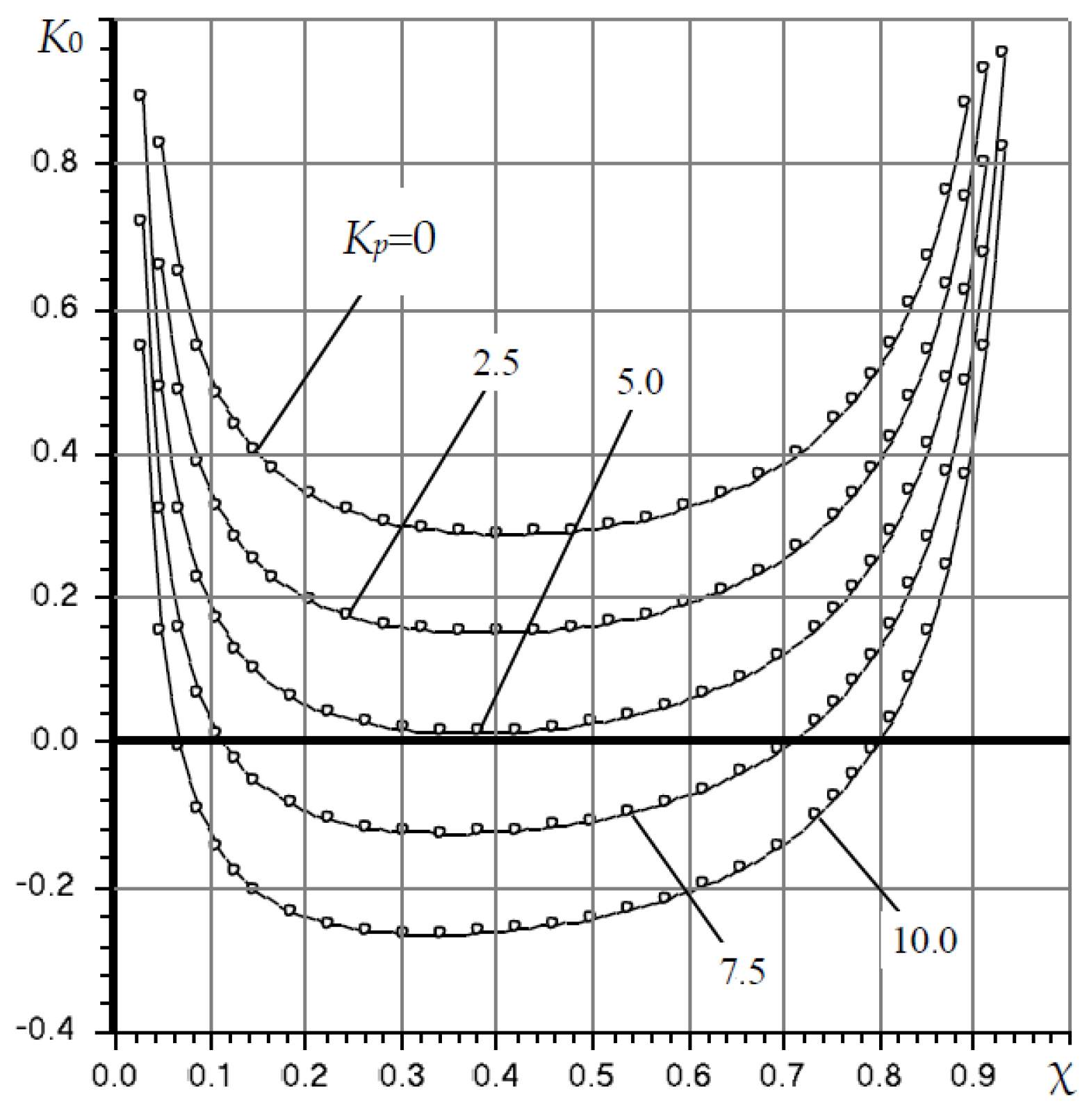
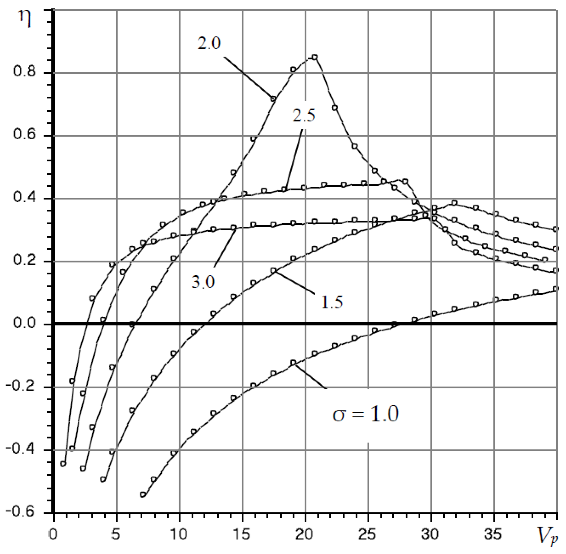
The dimensionless input parameters were used in the calculations: the mass of the shaft M = 1, the supply pressure P_S, the coefficient of adjusting the input slots’ resistance $\mathsf{\chi }=\left(P_{t0}^2-1\right)/\left(P_H^2-1\right)\in [0;1]$, the bearing half-length L, the ratios $p{L}_1=L_1/L\in (0;1)$, $p{L}_p=L_p/L_1\in (0;1)$, the outer radius R_p of the rings 5, the gap H_p0, the compliance K_p of the elastic rings 4, the number n of the finite-difference grid segments’ division, “squeeze number” σ and volume V_p. We found the gaps’ lengths L₁, L₂, L_p, pressure P_t0 and A_d parameter.

Static compliance K₀ = K(0) and the root quality criterion degree η of dynamic stability were considered to be criteria for bearing stability [14].

5. Research Results

The calculations showed that an acceptable relative error of 0.1% in the calculation of the criteria for the n number divisions of the integration segments in the c, t, p areas is ensured for n ≥ 8. Moreover, the order of CP $m=7(n-1)+3$. Therefore, for n = 8 the order is m = 52, for n = 16 the order is m = 108, etc., i.e., it can be in the tens or even hundreds. Figure 2 shows the location of CP zeros, where the abscissa axis corresponds to their real parts, and the ordinate axis corresponds to the imaginary parts. An analysis of the CP zeros arrangement showed that for the most part they are negative real numbers, and they are located at a great distance from the imaginary axis on the plane of the complex variable s values. Moreover, only 3–5 zeros are located near the imaginary axis, including zero with the largest real part, which determines the value of the criterion $\mathsf{\eta }$ (Figure 2a).

The calculation of the criterion η was carried out in two stages. In the first of them, the method of half division was used to find the mid-range (s ≥ –200) from the imaginary axis and the real zeros s_j of CP close to it, followed by dividing it by the difference (s–s_j). After such a “clearing” of the s plane at the second stage, by the Newton method [18] we searched for the zeros with the imaginary part remaining in this area (Figure 2b).

Figure 3 shows graphs of the bearing static compliance K₀. It can be seen that for the indicated set of parameter values, zero and negative compliance K₀ ≤ 0 takes place with the rings 4 material compliance K_p > 5 in the range of an adjusting coefficient 0.2 < χ < 0.6.

With the correct selection of the volume V_p, this bearing is as good in speed as a conventional bearing (K_p = 0, V_p = 0), which indicates the effectiveness of the damping chambers’ use to ensure the operability of the bearing with the regulation of the output flow rate.

The effect of the damping chambers volume V_p on the stability of the bearing can be assessed by the graphs in Figure 4. The comparison with the graphs in Figure 3 shows that in the absence of damping chambers (V_p = 0), the bearing is stable ($\mathsf{\eta }$ > 0) only with positive compliance K₀ > 0. With increasing values of this parameter, the bearing becomes stable even under zero and negative compliance modes (K₀ ≤ 0).

In addition to the parameter V_p, another important parameter, which affects only the quality of the bearing dynamics, is the “compression number” σ. Figure 5 shows the curves of the stability degree on these parameters. Function η(V_p, σ) is extreme, i.e., on the graph of this function there is a point that corresponds to the maximum speed of the bearing. For the given in Figure 5 parameters extremum of criterion η = 0.91 takes place at V_p = 24.6; σ = 2.1.

To verify the above calculations, the obtained data were compared with the static and dynamic characteristics of a conventional slotted radial bearing for the particular case K_p = 0 [19]. In terms of static characteristics, in particular compliance, the data coincide. There is an insignificant difference in the dynamic characteristics, which is explained by the fact that the compared data presented in [19] were obtained by a simplified method.

6. Conclusions

The results of the study allow us to conclude that a radial gas-static bearing with a limitation of the output gas flow rate can create zero and negative compliance. However, the operability of these structures can be ensured using special devices, which, as shown above, can be damping chambers located in the end area of the flow regulator.

At the same time, the active bearing and the conventional positive compliance bearing have a comparable dynamic quality. In the absence of vibration damping devices, an active bearing with zero and negative compliance is unstable.

It should also be noted that the application of the design approach based on the numerical finite-difference method to solve boundary-value problems for the linearized and transformed Reynolds equations to the study of the construction dynamics eliminated the issue of the calculation accuracy for the bearing stability criteria, which is a characteristic drawback of known approximate analytical methods.

References

1. Kodnyanko, V.; Shatokhin, S.; Kurzakov, A.; Pikalov, Y. Mathematical Modeling on Statics and Dynamics of Aerostatic Thrust Bearing with External Combined Throttling and Elastic Orifice Fluid Flow Regulation. Lubricants 2020, 8, 57. [Google Scholar] [CrossRef]
2. Kodnyanko, V.; Shatokhin, S.; Kurzakov, A.; Pikalov, Y. Theoretical analysis of compliance and dynamics quality of a lightly loaded aerostatic journal bearing with elastic orifices. Precis. Eng. 2021, 68, 72–81. [Google Scholar] [CrossRef]
3. Tkachev, A.; Kodnyanko, V. Two-row radial gas-static bearing with lubricant-outflow regulator. Russ. Eng. Res. 2009, 29, 926–929. [Google Scholar] [CrossRef]
4. Kodnyanko, V. Stability of an energy-saving adaptive radial hydrostatic bearing with restriction of lubricant output flow. J. Sib. Fed. Univ. Eng. Technol. 2011, 6, 674–684. [Google Scholar]
5. Bassani, R.; Ciulli, E.; Forte, P. Pneumatic stability of the integral aerostatic bearing: Comparison with other types of bearing. Tribol. Int. 1989, 22, 363–374. [Google Scholar] [CrossRef]
6. Jiunn-Yin, T. Feasibility Study of Super-Long Span Bridges Considering Aerostatic Instability by a Two-Stage Geometric Nonlinear Analysis. Int. J. Struct. Stab. Dyn. 2021, 21, 334. [Google Scholar] [CrossRef]
7. Kodnyanko, V.; Shatokhin, S. Theoretical study on dynamics quality of aerostatic thrust bearing with external combined throttling. FME Trans. 2020, 48, 342–350. [Google Scholar] [CrossRef]
8. Morosi, S.; Santos, I.F. Experimental Investigations of Active Air Bearings. In Proceedings of the ASME Turbo Expo 2012: Turbine Technical Conference and Exposition, Copenhagen, Denmark, 11–15 July 2012; pp. 901–910. [Google Scholar]
9. Wardle, F.P.; Bond, C.; Wilson, C.; Cheng, K.; Huo, D. Dynamic characteristics of a direct-drive air-bearing slide system with squeeze film damping. Int. J. Adv. Manuf. Technol. 2010, 47, 911–918. [Google Scholar] [CrossRef]
10. Sung, E.; Seo, C.-h.; Song, H.; Choi, B.; Jeon, Y.; Choi, Y.-M.; Kim, K.; Lee, M.G. Design and experiment of noncontact eddy current damping module in air bearing–guided linear motion system. Adv. Mech. Eng. 2019, 11, 1687814019871424. [Google Scholar] [CrossRef] [Green Version]
11. Zahorulko, A.; Lee, Y.-B. Dynamic behavior and difference pressure control of difference pressure regulator for dry gas seals. Mech. Syst. Signal. Process. 2022, 165, 108350. [Google Scholar] [CrossRef]
12. van der Wijngaart, W.; Berrier, A.; Stemme, G. A micropneumatic-to-vibration energy converter concept. Sens. Actuators A Phys. 2002, 100, 77–83. [Google Scholar] [CrossRef]
13. Constantinescu, V.N. Gas Lubrication; American Society of Mechanical Engineers: New York, NY, USA, 1969; p. 621. [Google Scholar]
14. Pinegin, S.; Tabachnikov, Y.; Sipenkov, I. Static and Dynamic Characteristics of Gas-Static Supports; Nauka: Moscow, Russia, 1982; p. 265. [Google Scholar]
15. Besekersky, V.; Popov, E. Theory of Automatic Control Systems; Elsevier: Saint Petersburg, Russia, 2003; p. 752. [Google Scholar]
16. Tanguy, J.-M. From Mathematical Model to Numerical Model. Numer. Methods 2013, 3, 31–58. [Google Scholar]
17. Kiusalaas, J. Numerical Methods in Engineering with MATLAB®; Cambridge University Press: Cambridge, UK, 2005. [Google Scholar] [CrossRef]
18. Mmbaga, J.; Nandakumar, K.; Hayes, R.; Flynn, M. Computational Methods for Engineers; ALPHA Education Press: Edmonton, AB, Canada, 2015; p. 335. [Google Scholar]
19. Stepanyants, L.; Zablotsky, N.; Sipenhov, I. Method of Theoretical Investigation of Externally Pressurized Gas-Lubricated Bearings. J. Lubr. Technol. 1969, 91, 166–170. [Google Scholar] [CrossRef]
Figure 1. The design scheme of the bearing.
Lubricants 09 00121 g001
Figure 2. The arrangement of characteristic polynomial zeros: (a)—original; (b)—corrected.
Lubricants 09 00121 g002
Figure 3. Dependences of the compliance K0 on the coefficient χ and compliance Kp of elastic rings at Ps = 4, L = 1.5, L1 = 0.3, Lp = 0.25, Rm = 1.2, Hp0 = 1.
Lubricants 09 00121 g003
Figure 4. Dependences of the stability degree η on the elastic rings’ compliance Kp and volume Vp at Ps = 4, χ = 0.5, L = 1.5, L1 = 0.3, Lp = 0.25, Rm = 1.2, Hp0 = 1; σ = 2.5.
Lubricants 09 00121 g004
Figure 5. Dependences of the stability degree η on the volume Vp and the “compression number” σ at Ps = 4, χ = 0.5, Kp = 10, L = 1.5, L1 = 0.3, Lp = 0.25, Rm = 1.2, Hp0 = 1.
Lubricants 09 00121 g005
Publisher’s Note: MDPI stays neutral with regard to jurisdictional claims in published maps and institutional affiliations.